Standard and Specific Compression Techniques for DNA Microarray Images


1
Department of Information and Communications Engineering, Building Q, Universitat Autònoma de Barcelona, Bellaterra, Cerdanyola del Vallès, 08193 Barcelona, Spain
2
Department of Electrical and Computer Engineering, The University of Arizona, 1230 E Speedway Blvd, Tucson, AZ 85721-0104AZ, USA
*
Author to whom correspondence should be addressed.
Algorithms 2012, 5(1), 30-49; https://doi.org/10.3390/a5010030
Submission received: 14 November 2011
/
Revised: 22 January 2012
/
Accepted: 22 January 2012
/
Published: 14 February 2012
(This article belongs to the Special Issue Data Compression, Communication and Processing)
Abstract
:We review the state of the art in DNA microarray image compression and provide original comparisons between standard and microarray-specific compression techniques that validate and expand previous work. First, we describe the most relevant approaches published in the literature and classify them according to the stage of the typical image compression process where each approach makes its contribution, and then we summarize the compression results reported for these microarray-specific image compression schemes. In a set of experiments conducted for this paper, we obtain new results for several popular image coding techniques that include the most recent coding standards. Prediction-based schemes CALIC and JPEG-LS are the best-performing standard compressors, but are improved upon by the best microarray-specific technique, Battiato’s CNN-based scheme.
1. Introduction
DNA microarray technology allows the analysis of the expression of thousands of genes in a single experiment and has become a very important tool in medicine and biology for the study of genetic function, regulation and interaction [1].Genome-wide monitoring is possible with existing DNA microarrays, which are used in research against cancer [2] and HIV [3], among many other applications.
DNA microarrays consist of a solid surface on which thousands of known genetic sequences are bound. Each sequence is placed in one microscopic hole or spot and all spots are arranged conforming to a regular pattern. Two samples, for example from healthy and tumoral tissue, are labeled, respectively, with green and red fluorescent markers called Cy3 and Cy5.Then, equal amounts of the labeled samples are made to react with the genetic sequences on the microarray. If one sample has an expressed sequence corresponding to a sequence placed in the microarray, part of it is hybridized and fixed in the correspondent spot; else, it gets washed away and will not be present in the spot. Once the hybridization and washing have concluded, the microarray is exposed to ultraviolet light so that the emissions from the fluorescent Cy3 and Cy5 dyes can be scanned and registered. Spots whose corresponding sequences are more strongly expressed in the first sample will have more Cy3 dye present and thus will emit more intense green light. The same can be said for the second sample and the red Cy5 dye. Comparing the relative intensity of the green and red channels, it is possible to detect which genes have not been equally expressed in both samples. This can be used to hypothesize about the function of individual genes under many different conditions.
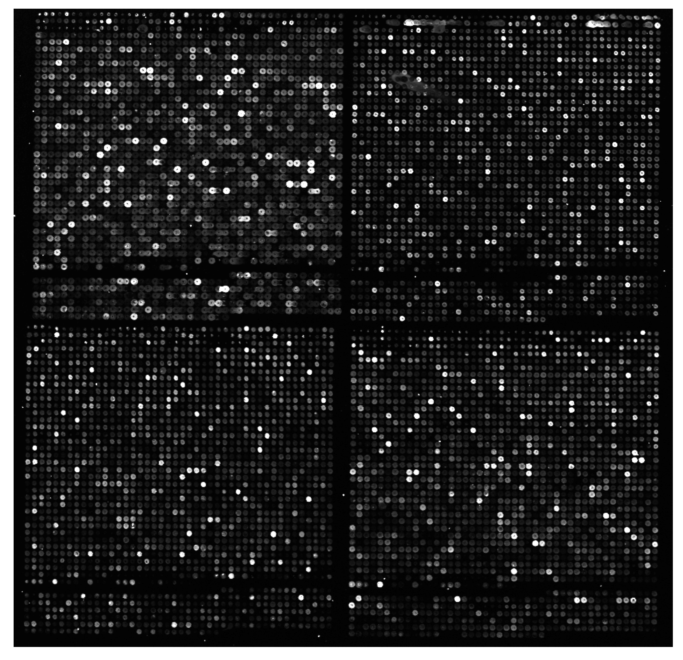
The output of a microarray experiment is a pair of monochrome images, one for the green channel and another for the red channel. An example microarray image can be seen in Figure 1. Due to the microscopic size of the spots, images have a high spatial resolution and are of large dimensions. Images from 1000 × 1000 onwards are described in the literature, but sizes over 4000 × 13000 are common nowadays. Since gene expression can vary in a very wide range, image pixel intensities have a depth of 16 bits per pixel (bpp).
Microarray images are computer analyzed to obtain genetic information. However, it is not desirable to keep only this genetic information and discard the microarray images. Analysis techniques are not fully mature or universally accepted and are subject to change. Furthermore, repeating an experiment is expensive and not always possible. Depending on the microarray size and the scanner spatial resolution, raw data for a single channel can require from a few to hundreds of Megabytes. With the increasing interest in DNA microarrays, and since many experiments are conducted under several different conditions, great amounts of data are generated in laboratories around the world. Because of the need of keeping and sharing microarray images, a need for efficient storage and transmission arises, and so compression emerges as a natural approach. The role of data compression in computational biology and the state of the art has been addressed by several authors [4,5].
Both lossy and lossless techniques have been proposed in the literature. Lossy approaches exhibit good compression performance on microarray images, but there is an open debate on whether information loss is acceptable or not, since it can alter genetic information extraction results. On the other hand, purely lossless methods guarantee immutable extraction results but offer poorer compression performance. This is partly due to the considerable amount of noise and the abundance of high frequencies present in this type of image.
This paper is structured as follows. In Section 2 we review compression schemes specific to microarray images including the most recent ones, and summarize their lossless compression results. In Section 3 we report a novel set of experiments that we have conducted using image compression standards, some of which had not been previously tested on DNA microarrays. Section 4 draws some conclusions.
2. State of the Art of DNA Microarray Image Compression
Image compression processes typically comprise up to 5 stages: preprocessing, transform, quantization, entropy coding and postprocessing. Microarray image compression can be modeled likewise. An exhaustive review of relevant works for microarray image compression published in the literature is provided in Subsections 2.1 to 2.7. Surveyed works are organized according to the stages where they make their contribution. This review extends the 2005 article by Luo and Lonardi [6] by addressing newer techniques that have appeared since then, and by providing a more complete and structured description. Compression results reported for all these techniques on different image sets used for benchmarking are compared in Subsection 2.8.
2.1.Preprocessing
The preprocessing stage comprises any computation performed on an image to prepare it for the compression or analysis processes. It is very important in DNA microarray images because many of the existing techniques rely heavily on the results of this stage to obtain competitive coding performance and to extract accurate genetic information. Denoising and segmentation are the main preprocessing techniques applied to this type of image, and are described next.
2.1.1. Denoising
Microarray images contain noise, which is sometimes considerable. This is due to imperfections in conducting the experiment and also in the image digitalization process. Being able to reduce noise can be useful to extract more accurate genetic information and to obtain better compression results. However, denoising-based compression is not lossless because denoising can be considered an irreversible transform that is applied before storing the image. There has been much research on denoising, but most of it is focused on the microarray analysis process and not on compression.
In 2006, Adjeroh et al. published their approach [7] based on the translation invariant (TI) transform. They argue that wavelet based denoising techniques that are not translation invariant suffer from an adverse pseudo-Gibbs phenomenon at discontinuities. This is especially important in microarray images since the edge of each spot can be considered a discontinuity. In their work, the original image is shifted horizontally, vertically and diagonally, and each of these shifted images plus the original one are denoised separately. The resulting images are then shifted back and combined to obtain the denoised image. Adjeroh et al. proposed three different approaches for combining the deshifted images: TI-hard, TI-median and TI-median2. The TI-hard method consists of outputting the average value of each pixel in the four deshifted images. The TI-median technique outputs the median instead of the average. The TI-median2 technique works by applying the TI-median technique twice: first, the TI-median is applied on the original image and an auxiliary image is produced; then the TI-median technique is applied again on the auxiliary image to obtain the denoised output image.
Many more authors have covered microarray image denoising for genetic information extraction, but only some of the most recent and relevant are referenced here. In 2005, Lukac proposed a method [8] based on fuzzy logic and local statistics for noise removal. Also in 2005, Smolka et al. discussed the peer group concept [9] as a means to remove impulsive noise. In 2007, Chen and Duan presented a simple method for denoising microarray images [10] based on comparing the edge features of the red and green channels. Recently, in 2010, Zifan et al. have designed multiwavelet transformations [11] to denoise images.
2.1.2. Segmentation
Segmentation, also know as spot finding or addressing, consists in determining which of the image pixels belong to spots (i.e., the foreground), as opposed to those that do not (i.e., the background). As will be discussed in Section 2.4, this can be very useful in later stages of the compression process. For example, it is possible to code separately foreground and background or to exploit differences in pixel intensity distributions between sets. We discuss here only specific approaches oriented towards image compression. However, for the sake of completeness, some segmentation techniques not directly focused on compression and some general segmentation quality metrics are described at the bottom of this subsection.
In 2003, Faramarzpour et al. proposed a lossless coder whose segmentation stage consists of two steps [12]. First, spot regions are located by studying the period of the signal obtained from summing the intensity by rows and by columns, and studying its minima. After that, spot centers are estimated based on the region centroid, which is needed for their spiral scanning procedure, as explained in Section 2.4. Simpler versions of this spot region location idea had already been used in microarray image analysis and also in Jörnsten and Yu’s work of 2002 [13], where they proposed a lossy-to-lossless compression scheme. In their technique, a seeded region growing algorithm is used to obtain a coarse mask for the spot pixels, which is then refined.
Later, in 2004, Lonardi and Luo presented their MicroZip lossy or lossless compression software [14]. They used a variation of Faramarzpour’s spot region finding idea, but they considered the existence of subgrids which are located before spot regions. Four subgrids can be appreciated in Figure 1, but other images may contain more.
In 2004, Hua et al. proposed a lossy or lossless scheme [15] with a segmentation technique based on the Mann–Whitney U test, which helps in deciding whether two independent sets of samples have equally large values. Once a region containing a spot has been located, a default mask is applied to obtain an initial set of pixels classified as spot pixels, and then the test is applied to add or remove pixels from this mask. This had already been used in microarray image segmentation [16], but the authors proposed a variation that speeds up the algorithm by up to 50 times.
Also in 2006, Bierman et al. described a purely lossless compression scheme [17] with a simple threshold method for dividing microarray images into low and high intensities. It consists of determining the lowest of the threshold values from 28, 29, 210 or 211 such that approximately 90% of the pixels fall within it.
In 2007, Neekabadi et al. proposed another threshold-based technique for segmentation [18], this time in three subsets: background, edge and spot pixels. Their lossless proposal performs segmentation in two steps. First, they determine the optimal threshold value by minimizing the total standard deviation of pixels above and below it. Then they segment the image in the mentioned subsets. To do so, first they determine the spot pixels by eroding the mask formed with pixels above the selected threshold. Edge pixels are the ones surrounding the spot pixels, and background pixels are all the others.
Finally in 2009, Battiato and Rundo published an approach [19] based on Cellular Neural Networks (CNNs). They define two layers for their lossless system, each with as many cells as the image has pixels. The input and state of the first layer are the pixels of the original image. Its output is the input and state of the second layer. By defining the cloning templates that drive the whole CNN dynamic, the second layer tends to its saturation equilibrium state and the resulting output tends to a “local binary image” where spot pixels tend to 1 and background pixels to 0.
Apart from the compression-oriented segmentation techniques already described, many others have been proposed in the more general context of DNA microarray image analysis. Some of the most recent are referenced next. In 2006, Battiato et al. proposed a microarray segmentation pipeline called MISP [20], where they used statistical region merging, γLUT and k-means clustering. In 2007, they improved the pipeline adding advanced image rotation and griding modules [21]. These two publications comprehensively describe previous well-known segmentation techniques. In 2008, Battiato et al. proposed a neurofuzzy segmentation strategy based on a Kohonen self-organizing map and an ulterior fuzzy k-means classifier [22]. In 2010, Karimi et al. described a new approach using an adaptive graph-based method [23]. Uslan et al. in 2010 [24] and Li et al. in 2011 [25] proposed two methods based on fuzzy c-means clustering. From the image-compression point of view, segmentation performance is generally measured based on the compression rates obtained after segmenting. However, in the DNA microarray image analysis context, other quality metrics might be applicable. In 2007, Battiato et al. defined a quality measure based on a previous technique for general DNA microarray image quality assessment, and compared the overall segmentation performances of their MISP technique and other previous approaches [21]. More information about microarray image quality assessment and information uncertainty can be found in Subsection 2.6.
2.2. Transform
The transform stage consists of changing the image domain from the spatial domain to another one where it can be more efficiently processed or coded. Examples of this are applying the DCT to obtain a frequency representation, or using a wavelet transform to change to the spatial-frequency domain.
However, wavelet-transform-based compression is not typically as efficient for microarray images as it is for other types of images [6]. For this reason, transformations are not frequently researched in microarray image compression, although they are used in some works. Since these papers provide little or no original contribution on the transformation stage, they are only briefly mentioned in this section.
In 2004, Hua et al. [15] published a modification of the EBCOT algorithm that included a tailored integer odd-symmetric transform for their proposed lossy or lossless scheme (see Section 2.4). In 2004, Lonardi and Luo [14] made use of the Burrows–Wheeler transform [26] for lossy or lossless compression in their MicroZip software (see Section 2.4). In 2006, Adjeroh et al. used a variation of the TI transform [7] for denoising (see Section 2.1). In 2007, Peters et al. [27] applied a slightly modified version of the singular value decomposition (SVD) in their lossy compression scheme (see Section 2.5). In 2010, Zifan et al. [11] used multiwavelet transformations, also for denoising (see Section 2.1). In 2011, Avanaki et al. [28] tested the use of an existing wavelet transform before applying fractal lossy compression (see Section 2.4).
2.3. Quantization
The stage of quantization consists of dividing sets of values or vectors into groups, effectively reducing the total number of symbols needed to represent them and thus increasing compressibility, at the expense of introducing information loss. In the microarray image compression literature, there are almost no original contributions for the quantization stage, partly because information loss is not always acceptable. There are however two exceptions.
In 2000 and in 2003 Jörnsten et al. [29,30] proposed both scalar and L1-norm vector adaptive quantizers (see Section 2.4) that can be used in lossy or lossless compression. In 2007, Peters et al. [27] used simple truncation in their lossy SVD-based technique (Section 2.5).
2.4. Entropy Coding
In this stage of the image compression process, data obtained from previous stages are expressed in an efficient manner to generate a more compact bitstream.
DNA microarray images show a strong spatial regularity [14], and this has been used in most techniques present in the literature. Many of them segment the image into foreground (spot) and background pixels and code them separately. Others build contexts or try to predict the intensity of the next pixels based on the previous ones, sometimes after segmenting the image.
Ideas following each of these patterns are discussed in the next two subsections. Some of the works could be classified in either or both of these groups. Here they have been assigned to the one that, in our opinion, is more important to the algorithm.
2.4.1. Segmentation Based Coding
DNA microarray images are usually segmented into spot and background pixels as part of the preprocessing stage to exploit their different statistical properties. Segmentation is always performed when extracting genetic information. Particular specific segmentation proposals have been discussed in Section 2.1. Several techniques that exploit this segmentation in their coding stage are presented next.
In 2002 and in 2003 Jörnsten et al. [13,29] presented a lossy-to-lossless compression scheme called SLOCO, a version of the LOCO-I algorithm, the basis of the JPEG-LS standard. After griding and segmentation, the image is divided into multiple rectangular subblocks, one for each spot. In this way, each spot can be accessed and sent independently and with different quality. For each spot subblock, two subimages are created: one where the background has been set to the spot mean value (the spot subimage), and another where the foreground has been set to the estimation of the background value so that the subimages have more homogeneous pixel intensities. Then each of the images is processed with SLOCO, which uses prediction in the spatial domain [31]. An important contribution of SLOCO is the use of an adaptive quantizer (UQ-adjust instead of UQ) that permits variable error per pixel δ so that spot pixels with higher intensities can be expressed with lower precision. Jörnsten et al. proposed both a scalar and a L1-norm vector quantizer (L1VQ), whose errors can be bitplane-encoded to obtain progressive lossy-to-lossless compression.
In 2003, Faramarzpour et al. presented a prediction-based lossless compression technique [12]. The image is gridded in rectangular subblocks, and spot centers are then estimated. For each of the subblocks, a spiral path is created to transform the 2D sequence into a 1D one. A linear prediction scheme that uses neighbor pixel intensities and their distances to the spot center is then applied on the 1D sequence. Differences between consecutive prediction errors form a sequence that is adaptive Huffman coded after being split on the index that minimizes the expected length of the coded sequences.
In 2004, Hua et al. presented microarray BASICA software [15] and proposed a progressive lossy-to-lossless compression scheme. In their work, they first grid and segment the image. After that, they separate each of the subblocks into foreground and background and then code them with a modified version of the EBCOT algorithm, the basis of the JPEG2000 standard [32]. The main modification to EBCOT is an adaptation of the original context modeling, which allows a better handling of the irregular shapes of the foreground and background subimages. Bit shifts are also performed when coding the foreground so that the most relevant information is sent first in this progressive scheme.
Also in 2004, Lonardi and Luo presented their MicroZip software [14], which offers both lossless and lossy compression. In their work, the image is first gridded and segmented into foreground and background. Then each of the 16-bit streams is divided into two 8-bit substreams comprising the most and least significant bytes. The four resulting substreams are losslessly coded except for the LSB of the background, which can be compressed either losslessly or with loss. Lossless coding is done using the Burrows–Wheeler Transform [26], originally designed for text compression, which reduces the total entropy by computing all permutations of a given channel and then sorting them lexicographically. Lossy coding is done with the SPIHT algorithm [33].
In 2006, Bierman et al. presented their lossless compression MACE (Micro Array Compression and Extraction) software [17]. In their work, high and low intensity pixels are separated using a simple threshold-based method to exploit the fact that intensity distribution in microarray images is very skewed. One image is generated for the low intensity pixels, and another for the high intensity ones. In the low intensity image, high intensity pixels are set to zero, and vice versa. The low intensity image is then losslessly coded using dictionary-based techniques such as Gzip or LZW, after being split into two subimages consisting of the most and least significant bytes of the original image, respectively. The high intensity image is processed with a sparse matrix algorithm, and then compressed. Later in 2007, Bierman et al. studied the performance impact of varying the dictionary size in their compression techniques [34]. They concluded that compression improved up to a certain dictionary size, where the performance stopped improving and began degrading.
In 2009, Battiato and Rundo published a lossless compression algorithm [19] based on image segmentation and color re-indexing. As previously discussed, segmentation is made by means of a CNN-based system and produces two complementary sub-images. The foreground is compressed with a generic lossless algorithm and stored separately. The background is first transformed into an indexed image. Then its color palette is re-indexed with an algorithm that reduces the zero-order entropy of local differences, which are losslessly coded. The re-indexing algorithm had been previously presented by the authors in 2007 [21].
2.4.2. Context-Based Coding
Contexts are used in image compression because they allow a more precise estimation of the occurrence probabilities of each symbol, which results in a reduction of the total entropy and thus of the compressed bitstream size.
In 2005 and in 2006 Zhang et al. [7,35] proposed a context-based lossless approach which also employed segmentation. In their work, they define a mixture model for microarray images where they consider two structural components (foreground and background) and assign probabilities based on the gamma distribution. Considering this model, they divide the image into two streams (foreground and background) and then each of those into two substreams, one for the most significant byte and the other for the least significant byte. MSB substreams are then processed by a simple predictive scheme, but LSB substreams are not. These four substreams are then coded with prediction by partial approximate matching (PPAM), a lossless compression technique also proposed by Zhang and Adjeroh [36]. In that paper, multicomponent compression is briefly addressed by compressing first one channel, Ir, and then the pixel by pixel difference, ID = Ir − Ig, obtaining slightly better results than compressing Ir and Ig separately.
In 2006, Neves and Pinho [37] proposed another context-based lossless approach. It is a bitplane-based technique that uses 3D finite-context models to drive an arithmetic coder. The most significant bitplane is encoded first, with a causal context formed by four surrounding pixels, and bitplanes from the second to the eighth most significant bitplanes are encoded using bits from the one being encoded and from the ones previously coded. Finally, the 8 least significant bitplanes are coded using only bits from the previous bitplanes for the context model. The probabilities used to drive the arithmetic coder are based on the number of times that a given symbol has appeared in the image while in a given context. The average coding bitrate for each bitplane is monitored and whenever one shows an expansive behavior (more than 1 bpp), that bitplane and the following bitplanes are not arithmetically coded, but simply output raw. Neves and Pinho used a trial and error procedure to build these context templates, which are the same for every image. In 2009, they extended this procedure so that specific templates are built for each image using a greedy approach, obtaining better results [38].
2.5. General Techniques Adapted to Microarray Images
Several authors have considered adapting generic image compression algorithms to DNA microarray images, as discussed previously. Others have opted to apply them directly, as described next.
2.6. Postprocessing
After compression, general images are sometimes processed to enhance their visual quality or to provide new features. DNA microarray images are not usually postprocessed with these goals. Rather, they are analyzed in order to extract genetic information and estimate their certainty. Because of this, traditional quality measures such as MSE or PSNR may not be completely suitable when performing lossy compression on DNA microarray images. Inspired by the manner in which genetic information is extracted, some researchers have proposed quality metrics specific for microarray images, which are applied after segmenting the image into spots and background.
Wang et al. proposed in 2001 a combined quality index (qcom), which considered spot sizes, signal to noise ratios, background variability and excessively high local background [39]. In 2004, Sauer et al. analyzed this metric and proposed and extended it to two new quality measures, qcom1 and qcom2 [40]. In 2005, Battiato et al. defined an image segmentation quality metric [21] based on the qcom2 measure. Pan-Gyu et al. defined another quality metric that considered signal and background noise, scale invariance, spot regularity and spot alignment [41]. Another factor to study is the information uncertainty of microarray experiments. It is common for DNA microarrays nowadays to replicate the same spot at least three times and to analyze the differences between the replicas to detect or alleviate the information variability of an experiment. Repeating an experiment using a number of different microarrays and comparing the information obtained for the same gene across them is another option to study the information uncertainty [23]. Different authors have used some of these concepts to define distortion measures for lossy microarray image compression, and have measured the performance of some of the discussed algorithms. The ideas on which these measures are sustained are described next.
2.6.1. Spot Detection
Spot detection consists of labeling spots as valid or invalid depending on a measure of the reliability of the extracted information. When performing lossy compression, this labeling might be affected, and thus one can define a distortion measure based on the number of differences in the classification [15].
2.6.2. Spot Identification
Spot identification consists of determining whether a particular gene is being expressed with higher, lower or the same intensity in the two samples that correspond to the two channels of a typical DNA microarray image. This is usually done by comparing pixel intensity properties of the two channels for each valid spot. Lossy compression can affect these pixel intensity properties, and thus one can define a distortion measure by counting the number of differences in the classification after compression [15,29], or even a quantitative difference between intensity logarithms [15].
2.6.3. Spot Classification
Once spots have been evaluated in the identification step, clustering algorithms are often applied to the measurements obtained for each spot in order to classify them into different groups. Hierarchical clustering and k-means are the most widely used algorithms for this purpose [7], but expression based classification has also been proposed [42]. The discrepancies between the classification or clustering results produced before and after lossy compression can be used to define new distortion measures.
2.6.4. Distortion Results
Despite the fact that several distortion measures have been defined, there are not many published surveys that report results for distortion measurements. The existing surveys consider mostly generic image compression techniques like SPIHT and JPEG2000, and the only algorithm specific to DNA microarray images studied in this context is SLOCO, Jörnsten’s algorithm [29,42,43].
Even though there seems to be significant reluctance to employ lossy compression, all authors that discuss distortion measures agree on the fact that for lossy compression, even at very low bitrates (high compression), these measures are affected in a very limited way [7,29,42]. Some claim that the variability induced by the lossy compression process is lower than that introduced when replicating an experiment [29], and even that lossy compression may improve the quality of the extracted information [7].
2.7. Technique Summary
All microarray-specific techniques reviewed above are summarized in Table 1 according to the subsections where they have been discussed. They have been sorted chronologically and marked as lossless, lossy, or both, depending on the type of compression in which they participate.
2.8. Lossless Compression Results Comparison
In this subsection, we first present image sets that have been used previously for benchmarking in the literature. Reported compression results for microarray-specific techniques are shown next. We analyze and compare those results to illustrate their relative compression performance for DNA microarray images. Lossy compression results are not discussed because published papers do not generally provide data tables that allow homogeneous comparisons among the different approaches, and also because it is not yet clear what an admissible information loss is. However, attending to the partial information available, it can be argued that lossy schemes which allow the compression with loss of the background with respect to the foreground are among the most frequent and successful.
2.8.1. Image Sets Used in the Literature
Several different image datasets have been used for benchmarking in microarray image compression, but none is common across all publications. In some papers, the images used are not specified. In others, only the source of the images is mentioned, but no other information about their size or characteristics is disclosed. Datasets that are described in the literature are presented in Table 2. Information about the number of images that they contain and their approximate size is also provided. Note that each image corresponds to one channel of a DNA microarray experiment.
2.8.2. Comparison of Results
Results from lossless compression schemes described in Section 2 are presented in Table 3. Techniques are listed chronologically, oldest first. Values for each algorithm and dataset are taken directly from the original papers. Dashes mean results were not provided for a given image set, and the Unspecified column is used when the image set is not revealed by the authors. Results are expressed in bits per pixel (bpp), so lower is better. Original images are all 16 bpp.
No single image set has been uniformly used for benchmarking in all techniques, so it is difficult to compare performance fairly. MicroZip, ApoA1 and ISREC are the sets that have been employed more frequently. Jörsten’s SLOCO claims the best results for the ApoA1 set with 8.556 bpp, but cannot be consistently compared to the other methods because of the lack of data for the other sets. With that exception, and attending only to the results for these three corpora, Battiato’s method based on CNNs performs best in all three with bitrates of 8.619 bpp, 9.52 bpp and 9.49 bpp, respectively. A lower bound of 8 bpp is believed to exist for microarray images due to the presence of random noise in the least
significant bitplanes. However, some authors have been able to obtain slightly better results for these bitplanes using high order contexts [35].
3. Compression Standards
It is important to compare microarray-specific techniques with generic compression techniques, especially standard techniques, in order to estimate the benefits of developing new microarray-specific techniques. In 2006, Pinho et al. [48] compared the performance of lossless JPEG2000, JBIG and JPEG-LS on the MicroZip, ApoA1 and ISREC image sets. We have conducted our own set of experiments and have been able to verify and extend their results.
In Subsection 3.1, all image sets used in our experiments (a superset of the sets used for benchmarking in the literature) are described. In Subsections 3.2 and 3.3 we report the compression performance results when using generic compression schemes and image compression standards, respectively.
3.1. Tested Image Sets
The MicroZip, Yeast, ApoA1 and ISREC sets used for benchmarking in the literature have been already described in Section 2.8. In addition, we have employed the Stanford set and the Arizona set. The Stanford set contains 20 images with sizes over 2000 × 2000, and up to 2200 × 2700, obtained from the Stanford Microarray Database public FTP at ftp://smd-ftp.stanford.edu/pub/smd/transfers/Jenny. The Arizona set has been kindly provided by David Galbraith and Megan Sweeney from the University of Arizona, and contains 6 images, each of size 4400 × 13800. All images are 16 bits per pixel. In Table 4, we summarize all the information about the different sets used in this work, including average image entropy.
3.2. General Compression Schemes
Results for general compressors (not image compressors) are shown in Table 5. These results have been computed dividing the total size in bits for all compressed files by the total number of pixels in the images. All compressors have been invoked in best compression mode. Best results in all datasets are obtained with Bzip2, which is especially efficient for the Yeast set.
3.3. Image Compression Standards
In our experiments we have tested the performance of standard image compression schemes as well. As in Pinho’s work, we have evaluated lossless JPEG2000, JBIG and JPEG-LS. In addition, we have examined results for CALIC and different modes for lossless JPEG2000. While Pinho et al. tested only the JJ2000 implementation using the default parameter selections of DWT, with 5 decomposition levels and 33 quality layers, we have also evaluated the performance with 0 to 5 decomposition levels and the same number of quality layers with both the JJ2000 and Kakadu implementations. We show in Table 6 an updated version of the data that we have previously provided [49]. As in the case of the general compression schemes, results are obtained by dividing the total number of bits of the compressed images by the total number of pixels of the original images.
We have obtained essentially identical results as in Pinho et al.’s work for the cases on which they have reported. Very similar results for all sets are obtained when using the Kakadu implementation with the same parameter choices used for JJ2000. In general, increasing the number of wavelet decomposition levels improves compression performance by approximately 0.5 bpp. The only exception is the Yeast set, where using 0 decomposition levels yields 32.33% better results than using 5 decomposition levels. A possible explanation is that the original images from the Yeast set contain less than 6% of all the possible intensities for a 16 bpp image, but applying one level of DWT produces three times as many different coefficient values and increases the entropy by more than 2 bits.
CALIC and JPEG-LS prediction-based schemes perform better than all the other non-specific schemes on all image sets except for the Yeast set, where JPEG2000 with 0 decomposition levels and JBIG significantly outperform CALIC in more than 23%. The best image compressor for each set is between 2.86% and 5.25% better than Bzip2, the best generic compressor. Battiato’s algorithm performs 12.81%, 10.45% and 11.85% better than the best non-microarray-specific technique for the MicroZip, ApoA1 and ISREC sets, respectively.
3.4. Image Properties Affecting Compression Performance
A key issue to be addressed when designing new compression schemes which improve overall performance could be identifying relevant image properties that affect the compression efficiency. Two different classes of properties can be defined for DNA microarray images: general properties applicable to any image and properties specific to microarray images.
General properties like resolution size or image entropy have the advantage of being more easily measurable, but also the disadvantage of not always providing much insight on the nature of DNA microarray images nor their compression. Image size does not correlate very well with the compression performance of any of the general or image-specific schemes shown in Table 3, Table 5 and Table 6. On the other hand, average entropy is clearly related to the compression performance for microarray images, but this fact is not useful for designing new algorithms.
Properties only applicable to DNA microarray images like spot quality and information uncertainty and their effect on compression could be very useful to understand the peculiarity of the underlying signal. Spot quality of microarray images and information uncertainty of microarray experiments (described in Subsection 2.6) may be useful in this regard. It would be very interesting to investigate the relationship of these two properties and the compression performance of different algorithms. Unfortunately, it is not feasible to do so in a straightforward way. Most quality assessment procedures rely on a previous segmentation of the image into foreground and background, but publicly available tools either require manual intervention, which is very inefficient and can cause imprecisions, or cannot be considered equally reliable for all datasets. Were an automatic method for assessing quality found, it would then be feasible to investigate the mentioned relationship. In addition, most information uncertainty measures require information of the genes associated to each spot, which is not available for the majority of the datasets used for benchmarking. If these data were available, it would be interesting to analyze the experimental deviations for the different datasets and their relationship with compression performance.
4. Conclusions and Future Work
DNA microarrays are state-of-the art tools widely used in biology and medicine. Analysis of microarray images is still being developed and repeating experiments is expensive or impossible, so keeping them for re-analysis is desirable. Due to the large amounts of data produced, efficient storage and transmission schemes are necessary, and compression arises as a natural approach. At least 10 compression schemes specific for microarray image compression have been proposed in the literature. We have classified all of them according to the stage or stages of the image compression process that they contribute to most, and have described their most relevant ideas.
Lossless compression results for both microarray-specific and different standard image compression methods have been discussed. The best microarray-specific technique reported for a variety of data sets is Battiato’s CNN-based proposal. According to our experiments, the best standard lossless image compressors are the prediction-based algorithms CALIC and JPEG-LS, except for the Yeast set, where lossless JPEG2000 with zero decomposition levels and JBIG improve upon those techniques. The best image compressor for each set is between 2.88% and 5.25% better than Bzip2 except for
the Yeast set, and Battiato’s algorithm performs 12.81%, 10.45% and 11.85% better than the best non-microarray-specific technique for the three image sets for which data from most algorithms exist.
As future work, we will analyze the properties of the new generation of DNA microarray scanners and their implications in the compression of the scanned images. We will also search for new data about the information uncertainty and image quality present in the different datasets, and analyze their relationship to compression performance.
Acknowledgments
The MicroZip corpus was kindly provided by Neves and Pinho from the University of Aveiro. The Arizona image set was provided by David Galbraith and Megan Sweeney from the University of Arizona.
This work has been partially supported by the European Union, by the Spanish Government (MICINN), by FEDER, and by the Catalan Government, under Grants FP7-PEOPLE-2009-IIFFP7-250420, TIN2009-14426-C02-01, FPU AP2010-0172, and 2009-SGR-1224.
References
- Moore, S. Making chips to probe genes. IEEE Spectr. 2001, 38, 54–60. [Google Scholar] [CrossRef]
- Satih, S.; Chalabi, N.; Rabiau, N.; Bosviel, R.; Fontana, L.; Bignon, Y.J.; Bernard-Gallon, D.J. Gene expression profiling of breast cancer cell lines in response to soy isoflavones using a pangenomic microarray approach. Omics J. Integr. Biol. 2010, 14, 231–238. [Google Scholar] [CrossRef]
- Giri, M.S.; Nebozhyn, M.; Showe, L.; Montaner, L.J. Microarray data on gene modulation by HIV-1 in immune cells: 2000–2006. J. Leukoc. Biol. 2006, 80, 1031–1043. [Google Scholar] [CrossRef]
- Nalbantoglu, O.U.; Russell, D.J.; Sayood, K. Data compression concepts and algorithms and their applications to Bioinformatics. Entropy 2010, 12, 34–52. [Google Scholar] [CrossRef] [PubMed]
- Giancarlo, R.; Scaturro, D.; Utro, F. Textual data compression in computational biology: A synopsis. Bioinformatics 2009, 25, 1575–1586. [Google Scholar] [CrossRef] [PubMed]
- Luo, Y.; Lonardi, S. Storage and transmission of microarray images. Drug Discov. Today 2005, 10, 1689–1695. [Google Scholar] [CrossRef]
- Adjeroh, D.A.; Zhang, Y.; Parthe, R. On denoising and compression of DNA microarray images. Pattern Recogn. 2006, 39, 2478–2493. [Google Scholar] [CrossRef]
- Lukac, R.; Plataniotis, K.; Smolka, B.; Venetsanopoulos, A. A Data-Adaptive Approach to cDNA Microarray Image Enhancement. In Proceedings of the International Conference on Computational Science (ICCS ’05), Atlanta, GA, USA, 22–25 May 2005; pp. 886–893. [Google Scholar]
- Smolka, B.; Plataniotis, K. Ultrafast Technique of Impulsive Noise Removal With Application To Microarray Image Denoising. In Proceedings of the Image Analysis and Recognition, Toronto, ON, Canada, September 2005; Kamel, M., Campilho, A., Eds.; Springer-Verlag: Berlin, Germany, 2005; Volume 3656, pp. 990–997. [Google Scholar]
- Chen, X.; Duan, H. A Vector-Based Filtering Algorithm for Microarray Image. In Proceedings of the IEEE/ICME International Conference on Complex Medical Engineering, Beijing, China, 23–27 May 2007; Volume 1–4, pp. 794–797. [Google Scholar]
- Zifan, A.; Moradi, M.H.; Gharibzadeh, S. Microarray image enhancement by denoising using decimated and undecimated multiwavelet transforms. Signal Image Video Process. 2010, 4, 177–185. [Google Scholar] [CrossRef]
- Faramarzpour, N.; Shirani, S.; Bondy, J. Lossless DNA microarray image compression. In Proceedings of the 37th Asilomar Conference on Signals, Systems and Computers; 2003; Volume 2, pp. 1501–1504. [Google Scholar]
- Jornsten, R.; Vardi, Y.; Zhang, C. On the Bitplane Compression of Microarray Images. In Proceedings of the 4th International Conference on Statistical Data Analysis Based on the L1-Norm and Related Methods, Neuch’tel, Switzerland, 4–9 August 2002. [Google Scholar]
- Lonardi, S.; Luo, Y. Gridding and Compression of Microarray Images. In Proceedings of the IEEE Computational Systems Bioinformatics Conference, Stanford, CA, USA, 16–19 August 2004; pp. 122–130. [Google Scholar]
- Hua, J.; Liu, Z.; Xiong, Z.; Wu, Q.; Castleman, K. Microarray BASICA: Background adjustment, segmentation, image compression and analysis of microarray images. EURASIP J. Appl. Signal Process. 2004, 2004, 92–107. [Google Scholar] [CrossRef]
- Chen, Y.; Dougherty, E.R.; Bittner, M.L. Ratio-based decisions and the quantitative analysis of cDNA microarray images. J. Biomed. Opt. 1997, 2, 364–374. [Google Scholar] [CrossRef]
- Bierman, R.; Maniyar, N.; Parsons, C.; Singh, R. MACE: Lossless Compression and Analysis of Microarray Images. In Proceedings of the ACM Symposium on Applied Computing (SAC ’06), Dijon, France, 23–27 April 2006; pp. 167–172. [Google Scholar]
- Neekabadi, A.; Samavi, S.; Razavi, S.A.; Karimi, N.; Shirani, S. Lossless Microarray Image Compression Using Region Based Predictors. In Proceedings of the International Conference on Image Processing, San Antonio, TX, USA, 16 September–19 October 2007; Volume 1–7, pp. 913–916. [Google Scholar]
- Battiato, S.; Rundo, F. A Bio-Inspired CNN With Re-Indexing Engine for Lossless DNA Microarray Compression and Segmentation. In Proceedings of the 16th International Conference on Image Processing, Cairo, Egypt, 7–10 November 2009; Volume 1–6, pp. 1717–1720. [Google Scholar]
- Battiato, S.; Blasi, G.D.; Farinella, G.M.; Gallo, G.; Guarnera, G.C. Ad-hoc segmentation pipeline for microarray image analysis. Proc. SPIE 2006, 6064, 300–311. [Google Scholar]
- Battiato, S.; Rundo, F.; Stanco, F. Self organizing motor maps for color-mapped image re-indexing. IEEE Trans. Image Process. 2007, 16, 2905–2915. [Google Scholar] [CrossRef] [PubMed]
- Battiato, S.; Farinella, G.; Gallo, G.; Guarnera, G. Neurofuzzy Segmentation of Microarray Images. In Proceedings of the 19th International Conference on Pattern Recognition (ICPR ’08), Tampa, FL, USA, 8–11 December 2008; pp. 1–4. [Google Scholar]
- Karimi, N.; Samavi, S.; Shirani, S.; Behnamfar, P. Segmentation of DNA microarray images using an adaptive graph-based method. IET Image Process. 2010, 4, 19–27. [Google Scholar] [CrossRef]
- Uslan, V.; Bucak, I.O. Clustering-Based Spot Segmentation of cDNA Microarray Images. In Proceedings of the 2010 Annual International Conference of the IEEE Engineering in Medicine and Biology Society (EMBC), Buenos Aires, Argentina, 31 August–4 September 2010; pp. 1828–1831. [Google Scholar]
- Li, Z.; Weng, G. Segmentation of cDNA Microarray Image using Fuzzy c-mean Algorithm and Mathematical Morphology. Key Engineering Materials 2011, 464, 159–162. [Google Scholar] [CrossRef]
- Burrows, M.; Wheeler, D.J. A Block-Sorting Lossless Data Compression Algorithm. Technical Report 124; HP: Palo Alto, CA, USA, 1994. [Google Scholar]
- Peters, T.J.; Smolikova-Wachowiak, R.; Wachowiak, M.P. Microarray Image Compression Using a Variation of Singular Value Decomposition. In Proceedings of the Annual International Conference of the IEE Engineering in Medicine and Biology Society, Lyon, France, 22–26 August 2007; Volume 1–16, pp. 1176–1179. [Google Scholar]
- Avanaki, M.R.N.; Aber, A.; Ebrahimpour, R. Compression of cDNA microarray images based on pure-fractal and wavelet-fractal techniques. ICGST Int. J. Graph. Vis. Image Process. GVIP 2011, 11, 43–52. [Google Scholar]
- Jornsten, R.; Wang, W.; Yu, B.; Ramchandran, K. Microarray image compression: SLOCO and the effect of information loss. Signal Process. 2003, 83, 859–869. [Google Scholar] [CrossRef]
- Jornsten, R.; Yu, B. “Comprestimation”: Microarray Images in Abundance. In Proceedings of the Conference on Information Sciences and Systems, Princeton, NJ, USA, 15–17 March 2000. [Google Scholar]
- Weinberger, M.J.; Seroussi, G.; Sapiro, G. The LOCO-I lossless image compression algorithm: Principles and standardization into JPEG-LS. IEEE Trans. Image Process. 2000, 9, 1309–1324. [Google Scholar] [CrossRef]
- Taubman, D.S.; Marcellin, M.W. JPEG2000: Image Compression Fundamentals, Standards and Practice; Kluwer Academic Publishers: Boston, MA, USA, 2002. [Google Scholar]
- Said, A.; Pearlman, W.A. A new fast and efficient image codec based on set partitioning in hierarchical trees. IEEE Trans. Circuits Syst. Video Technol. 1996, 6, 243–250. [Google Scholar] [CrossRef]
- Bierman, R.; Singh, R. Influence of Dictionary Size on the Lossless Compression of Microarray Images. In Proceedings of the 20th International Symposium on Computer-Based Medical Systems, Maribor, Yugoslavia, 20–22 June 2007; Kokol, P., Podgorelec, V., MiceticTurk, D., Zorman, M., Verlic, M., Eds.; pp. 237–242. [Google Scholar]
- Zhang, Y.; Parthe, R.; Adjeroh, D. Lossless Compression of DNA Microarray Images. In Proceedings of the IEEE Computational Systems Bioinformatics Conference, Stanford, CA, USA, 8–11 August 2005; pp. 128–132. [Google Scholar]
- Zhang, Y.; Adjeroh, D. Prediction by partial approximate matching for lossless image compression. IEEE Trans. Image Process. 2008, 17, 924–935. [Google Scholar] [CrossRef]
- Neves, A.J.R.; Pinho, A.J. Lossless Compression of Microarray Images. In Proceedings of the International Conference on Image Processing, ICIP, Atlanta, CA, USA, 8–11 August 2006; pp. 2505–2508. [Google Scholar]
- Neves, A.J.R.; Pinho, A.J. Lossless compression of microarray images using image-dependent finite-context models. IEEE Trans. Med. Imaging 2009, 28, 194–201. [Google Scholar] [CrossRef]
- Wang, X.; Ghosh, S.; Guo, S.W. Quantitative quality control in microarray image processing and data acquisition. Nucleic Acids Res. 2001, 29, e75. [Google Scholar] [CrossRef] [PubMed]
- Sauer, U.; Preininger, C.; Hany-Schmatzberger, R. Quick and simple: Quality control of microarray data. Bioinformatics 2004, 21, 1572–1578. [Google Scholar] [CrossRef] [PubMed]
- Kim, P.G.; Park, K.; Cho, H.G. A quality measure model for microarray images. Int. J. Inf. Technol. 2005, 11, 117–124. [Google Scholar]
- Xu, Q.; Hua, J.; Xiong, Z.; Bittner, M.L.; Dougherty, E.R. The effect of microarray image compression on expression-based classification. Signal Image Video Process. 2009, 3, 53–61. [Google Scholar] [CrossRef]
- Xu, Q.; Hua, J.; Xiong, Z.; Bittner, M.; Dougherty, E. Accuracy of Differential Expression Detection With Compressed Microarray Images. In Proceedings of the International Workshop on Genomic Signal Processing and Statistics (GENSIPS ’06), College Station, TX, USA, 28–30 May 2006; pp. 43–44. [Google Scholar]
- Lonardi, S.; Luo, Y. MicroZip microarray image set. Available online: http://www.cs.ucr.edu/yuluo/MicroZip/ (accessed November 2011).
- Stanford Yeast Cell-Cycle Regulation Project. Yeast microarray image set. Available online: http://genome-www.stanford.edu/cellcycle/data/rawdata/individual.html (accessed on November 2011).
- Terry Speed Microarray data analysis group. ApoA1 microarray image set. Available online: http://www.stat.berkeley.edu/users/terry/zarray/Html/apodata.html (accessed on November 2011).
- Swiss Institute for Bioinformatics (SIB). ISREC microarray image set. Available online: http://www.isrec.isb-sib.ch/DEA/module8/P5 chip image/images/ (accessed on November 2011).
- Pinho, A.; Paiva, A.; Neves, A. On the use of standards for microarray lossless image compression. IEEE Trans. Biomed. Eng. 2006, 53, 563–566. [Google Scholar] [CrossRef]
- Herna´ndez-Cabronero, M.; Blanes, I.; Serra-Sagristaá, J.; Marcellin, M.W. A Review of DNA Microarray Image Compression. In Proceedings of the IEEE International Conference on Data Compression, Communication and Processing, CCP, Palinuro, Italy, 21–24 June 2011; pp. 139–147. [Google Scholar]
Figure 1.
940 × 910 portion of red channel image y744n43 ch2.tif from the Yeast dataset. Gamma levels have been adjusted in the figure for better viewing.
Figure 1.
940 × 910 portion of red channel image y744n43 ch2.tif from the Yeast dataset. Gamma levels have been adjusted in the figure for better viewing.


Table 1.
Classification of microarray-specific techniques discussed in this document, attending to the compression stage where they make their contribution. Techniques are sorted chronologically and can appear in more than one category. Purely lossy methods are marked with red and ×. Purely lossless with blue and ☐. Lossy and lossless with green and ⊠.
| Preprocessin | Transform Quantization | Entropy coding | Generic | Postprocessing | |||
|---|---|---|---|---|---|---|---|
| Denoising | Segmentation | Segmentation | Context | ||||
| × [8], 2005 | ⊠ [13], 2002 | ⊠ [15], 2004 | × [30], 2000 | ⊠ [13], 2002 | ☐ [35], 2005 | × [27], 2007 | ⊠ [29], 2003 |
| × [9], 2005 | ☐ [12], 2003 | ⊠ [14], 2004 | ⊠ [29], 2003 | ⊠ [29], 2003 | ☐ [7], 2006 | × [28], 2011 | ⊠ [15], 2004 |
| × [7], 2006 | ⊠ [15], 2004 | ☐ [7], 2006 | × [27], 2007 | ☐ [12], 2003 | ☐ [37], 2006 | × [7], 2006 | |
| × [10], 2007 | ⊠ [14], 2004 | × [27], 2007 | ⊠ [15], 2004 | ☐ [38], 2009 | ⊠ [42], 2009 | ||
| × [11], 2010 | ☐ [17], 2006 | × [11], 2010 | ⊠ [14], 2004 | ||||
| ☐ [18], 2007 | × [28], 2011 | ☐ [17], 2006 | |||||
| ☐ [19], 2009 | ☐ [34], 2007 | ||||||
| ☐ [21], 2007 | |||||||
| ⊠ [19], 2009 | |||||||
Table 2.
Image sets referenced in the literature. All images are 16 bpp.
| Dataset | Images | Size (px) |
|---|---|---|
| MicroZip [44] | 3 | > 1800 × 1900 |
| Yeast [45] | 109 | 1024 × 1024 |
| ApoA1 [46] | 32 | 1044 × 1041 |
| ISREC [47] | 14 | 1000 × 1000 |
Table 3.
Comparison of lossless microarray-specific schemes on 16 bpp images. All results are expressed in bits per pixel (bpp), so lower is better. All results have been adopted directly from the references specified in the table. Best results for each specified image set have been highlighted in green, and worst results in red.
| Algorithm | Year | MicroZip | Yeast | ApoA1 | ISREC | Unspecified |
|---|---|---|---|---|---|---|
| SLOCO [13] | 2002 | — | — | 8.556 | — | — |
| Faramarzpour [12] | 2003 | — | — | — | — | 9.091 |
| Hua [15] | 2004 | — | — | — | — | 6.985 |
| MicroZip [14] | 2004 | 9.843 | — | — | — | — |
| PPAM [35] | 2005 | 9.587 | 6.601 | — | — | — |
| MACE [17] | 2006 | — | — | — | — | 7.070 |
| Neves [37] | 2006 | 8.840 | — | 10.280 | 10.199 | — |
| Neekabadi [18] | 2007 | 8.856 | — | 10.250 | 10.202 | — |
| Battiato [19] | 2009 | 8.369 | — | 9.52 | 9.49 | — |
| Neves [38] | 2009 | 8.619 | — | 10.194 | 10.158 | — |
Table 4.
Image sets used in the literature and in this work. All images are 16 bpp.
| Image set | Images | Size (px) | Average entropy (bpp) |
|---|---|---|---|
| MicroZip | 3 | > 1,800 × 1,900 | 9.831 |
| Yeast | 109 | 1, 024 × 1, 024 | 6.628 |
| ApoA1 | 32 | 1, 044 × 1, 041 | 11.033 |
| ISREC | 14 | 1, 000 × 1, 000 | 10.435 |
| Stanford | 20 | > 2, 000 × 2, 000 | 8.293 |
| Arizona | 6 | 4, 400 × 13, 800 | 9.306 |
Table 5.
Lossless compression results in bpp for general (not image compressors nor microarray-specific) entropy coders and individual image compression, using the best compression invocation parameters, obtained by the authors. All images are 16 bpp. Best results are highlighted in green and worst results in red.
| Algorithm | MicroZip | Yeast | ApoA1 | ISREC | Stanford | Arizona |
|---|---|---|---|---|---|---|
| Gzip (LZ77) | 11.426 | 7.548 | 12.711 | 12.462 | 9.813 | 11.032 |
| AC (16-bit symbols) | 11.011 | 7.688 | 12.531 | 12.011 | 9.564 | 10.398 |
| XZ (LZMA2) | 9.696 | 6.385 | 11.321 | 11.015 | 8.163 | 9.284 |
| Bzip2 | 9.394 | 6.075 | 11.067 | 10.921 | 7.867 | 8.944 |
Table 6.
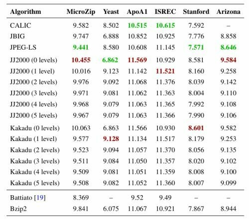
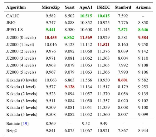
Lossless compression results in bpp for generic (not microarray-specific) image compressors and individual image compression, obtained by the authors. Standard compression parameters have been used for all algorithms except for JPEG2000, where different DWT decomposition levels have been applied. All images are 16 bpp. Best results are highlighted in green and worst results in red. Results for the best microarray-specific technique and the best general compressor are repeated at the bottom for ease of reference.
Table 6.
Lossless compression results in bpp for generic (not microarray-specific) image compressors and individual image compression, obtained by the authors. Standard compression parameters have been used for all algorithms except for JPEG2000, where different DWT decomposition levels have been applied. All images are 16 bpp. Best results are highlighted in green and worst results in red. Results for the best microarray-specific technique and the best general compressor are repeated at the bottom for ease of reference.
| Algorithm | MicroZip | Yeast | ApoA1 | ISREC | Stanford | Arizona |
|---|---|---|---|---|---|---|
| CALIC | 9.582 | 8.502 | 10.515 | 10.615 | 7.592 | – |
| JBIG | 9.747 | 6.888 | 10.852 | 10.925 | 7.776 | 8.858 |
| JPEG-LS | 9.441 | 8.580 | 10.608 | 11.145 | 7.571 | 8.646 |
| JJ2000 (0 levels) | 10.064 | 6.862 | 11.569 | 10.929 | 8.581 | 9.584 |
| JJ2000 (1 level) | 9.583 | 9.123 | 11.142 | 11.521 | 8.160 | 9.258 |
| JJ2000 (2 levels) | 9.530 | 9.092 | 11.068 | 11.376 | 8.039 | 9.142 |
| JJ2000 (3 levels) | 9.519 | 9.081 | 11.062 | 11.363 | 8.004 | 9.110 |
| JJ2000 (4 levels) | 9.517 | 9.079 | 11.063 | 11.365 | 7.992 | 9.108 |
| JJ2000 (5 levels) | 9.515 | 9.079 | 11.063 | 11.366 | 7.990 | 9.106 |
| Kakadu (0 levels) | 10.063 | 6.863 | 11.566 | 10.930 | 8.601 | 9.582 |
| Kakadu (1 level) | 9.577 | 9.128 | 11.134 | 11.517 | 8.179 | 9.253 |
| Kakadu (2 levels) | 9.523 | 9.094 | 11.057 | 11.370 | 8.056 | 9.135 |
| Kakadu (3 levels) | 9.511 | 9.084 | 11.050 | 11.357 | 8.020 | 9.102 |
| Kakadu (4 levels) | 9.509 | 9.081 | 11.051 | 11.359 | 8.008 | 9.100 |
| Kakadu (5 levels) | 9.508 | 9.082 | 11.052 | 11.360 | 8.007 | 9.099 |
| Battiato [19] | 8.369 | – | 9.52 | 9.49 | – | – |
| Bzip2 | 9.394 | 6.075 | 11.067 | 10.921 | 7.867 | 8.944 |
Publisher’s Note: MDPI stays neutral with regard to jurisdictional claims in published maps and institutional affiliations. |
© 2012 by the authors. Licensee MDPI, Basel, Switzerland. This article is an open access article distributed under the terms and conditions of the Creative Commons Attribution (CC BY) license (https://creativecommons.org/licenses/by/4.0/).
Share and Cite
MDPI and ACS Style
Hernández-Cabronero, M.; Blanes, I.; Marcellin, M.W.; Serra-Sagristà, J. Standard and Specific Compression Techniques for DNA Microarray Images. Algorithms 2012, 5, 30-49. https://doi.org/10.3390/a5010030
AMA Style
Hernández-Cabronero M, Blanes I, Marcellin MW, Serra-Sagristà J. Standard and Specific Compression Techniques for DNA Microarray Images. Algorithms. 2012; 5(1):30-49. https://doi.org/10.3390/a5010030
Chicago/Turabian StyleHernández-Cabronero, Miguel, Ian Blanes, Michael W. Marcellin, and Joan Serra-Sagristà. 2012. "Standard and Specific Compression Techniques for DNA Microarray Images" Algorithms 5, no. 1: 30-49. https://doi.org/10.3390/a5010030