An Agent-Based Fuzzy Collaborative Intelligence Approach for Predicting the Price of a Dynamic Random Access Memory (DRAM) Product

Abstract

Predicting the price of a dynamic random access memory (DRAM) product is a critical task to the manufacturer. However, it is not easy to contend with the uncertainty of the price. In order to effectively predict the price of a DRAM product, an agent-based fuzzy collaborative intelligence approach is proposed in this study. In the agent-based fuzzy collaborative intelligence approach, each agent uses a fuzzy neural network to predict the DRAM price based on its view. The agent then communicates its view and forecasting results to other agents with the aid of an automatic collaboration mechanism. According to the experimental results, the overall performance was improved through the agents’ collaboration.

1. Introduction

Dynamic random access memory (DRAM) manufacturing is a very competitive industry. If a DRAM manufacturer is unable to grasp the future price changes, then it may fail because of the substantial losses. Tarui and Tarui [1] found that for DRAM long-term trends do exist and could be approximately modeled. The same phenomenon can also be observed in other industries [2,3,4,5,6,7,8,9,10]. Cupertino [11] was not so optimistic. He claimed that only the turning points in the semiconductor industry could be anticipated somehow. Instead of directly observing price, Grimm [12] and Aizcorbe [13] both proposed quality-adjusted price indexes for some semiconductor devices. Triplett [14] proposed a hedonic price index for some semiconductor products formed from an envelope of demand and supply functions for individual buyers and sellers. Overall, the market for DRAM is highly cyclical. The oversupply of DRAM in the market drives DRAM prices downward. At the same time, there is additional price pressure from personal computer manufacturers. These situations sometimes result in the price of a DRAM product dipping below its production cost, making for a very difficult business environment. In short, there are numerous factors that will affect the price of DRAM [15]. Although it is impossible to consider all these factors at the same time, if we can model DRAM price as a function of some of them, then the function can be used to predict DRAM price. Another common practice is to consider DRAM price changes as a time series, so as to infer the future DRAM price from the historical values. Attempts in this field dated back to Lepselter and Sze [16], in which the π rule is proposed, which described the trend in the average price of packaged DRAM chips as a logarithmic function of time. The π rule states that in the face of rapid price decreases, the peak volume of chips shipped corresponds to a per-chip price of π dollars. The price continues to decline and eventually settles at about π/2 dollars per chip. This nicely described the trends in the prices of DRAMs up to 64 K. Subsequently, Tarui and Tarui [1] modified the π rule and proposed the Bi-rule by considering the fact that bit cost would be reduced by one half with each succeeding DRAM generation. The trends in the prices of DRAMs up to 16 M indeed reflected this fact. However, for DRAMs manufactured with much more advanced technologies, these simple rules did not work very well.

In Chen and Wang [17], some experts predicted the price of a DRAM product during some future periods with fuzzy values, which are then interpolated to determine the prices of the other periods. Such a way is subjective, and suffers from the accumulation in the fuzziness. Ong et al. [18] optimized the configuration of the auto-regressive integrated moving average (ARIMA) approach with a genetic algorithm (GA), and applied it to predict the price of a DRAM product. Chen [15] employed the fuzzy ARIMA (FARIMA) approach proposed by Tseng et al. [19] to accomplish the same task.

In addition, in some occasions, the range covering the actual value needs to be estimated for various managerial purposes. This means the precision of DRAM price forecasting must be elevated as well. Recently, Chen [20] employed the fuzzy linear regression and back propagation network (FLR-BPN) approach that reflected such considerations.

On the other hand, with the widespread array of Internet applications, dealing with disparate data sources is becoming increasingly popular. Furthermore, due to technical limitations, security or privacy considerations, the integral access to a number of sources is often limited [21,22]. For these reasons, Pedrycz [22] proposed the concepts of collaborative computing intelligence and collaborative fuzzy modeling, and developed the so-called fuzzy collaborative system. However, most existing fuzzy collaboration systems are used for clustering, the so-called fuzzy collaborative clustering system [23,24].

This study is aimed at developing an agent-based fuzzy collaborative intelligence approach for forecasting the price of a DRAM product. Fuzzy collaborative forecasting systems for similar purposes have rarely been discussed in the literature, yet they have great potential [25,26,27,28,29,30,31,32,33]. The remainder of this paper is arranged in the following manner. Section 2 provides the details of the agent-based fuzzy collaborative intelligence approach. In Section 3, a real case is used to evaluate the effectiveness of the agent-based fuzzy collaborative intelligence approach. The performances of some existing methods in this field are also examined for a comparison. Section 4 concludes this paper and points out some interesting topics for future work.

2. Methodology

The operating procedure of the agent-based fuzzy collaborative intelligence approach consists of several steps that will be described in the following sections:

(1) The agent-based fuzzy collaborative intelligence approach starts from the formation of the agent group.

(2) Each agent automatically determines the setting 23 of the fuzzy back propagation network (FBPN) reasoning module associated with the agent.

(3) Each agent predicts the DRAM price based on the agent’s view.

(4) Each agent communicates its view and forecasting results to other agents with the aid of the automatic collaboration mechanism. Upon receipt, the agent adjusts its setting, so as to improve the overall performance.

(5) To aggregate the forecasting results, a radial basis function (RBF) network is employed by the automatic collaboration mechanism.

(6) The collaboration process is terminated if the improvement in the forecasting performance becomes negligible. Otherwise, return to step (4).

In the agent-based fuzzy collaborative intelligence approach, each agent uses a FBPN to predict the DRAM price. Although there have been some more advanced artificial neural networks, such as the compositional pattern-producing network, cascading neural network, dynamic neural network, and others, a well-trained FBPN with an optimized structure can still produce very good results, which is why it is selected for this study:

(1) Inputs: K inputs, corresponding to the prices K months ago. To facilitate the search for solutions, it is strongly recommended to normalize the inputs to a range narrower than [0 1]:

$$\mathit{N}(\mathit{x})={\mathit{N}}_{\mathit{L}}+\frac{\mathit{x}-{\mathit{x}}_{\min }}{{\mathit{x}}_{\max \mathrm{-}}{\mathit{x}}_{\min }}·({\mathit{N}}_{\mathit{U}}-{\mathit{N}}_{\mathit{L}})$$

(1)

where N(x) is the normalized value of x; N_L and N_U indicate the lower and upper bounds of the range of the normalized value, respectively. x_min and x_max are the minimum and maximum of x, respectively. The formula can be written as

$$\mathit{x}=\frac{\mathit{N}\mathrm{(}\mathit{x}\mathrm{)}-{\mathit{N}}_{\mathit{L}}}{{\mathit{N}}_{\mathit{U}}-{\mathit{N}}_{\mathit{L}}}·\mathrm{(}{\mathit{x}}_{\max \mathrm{-}}{\mathit{x}}_{\min }\mathrm{)}+{\mathit{x}}_{\min }$$

(2)

if the un-normalized value is to be obtained instead.

(2) The FBPN has only one hidden layer, which can approximate arbitrarily any function that contains a continuous mapping from one finite space to another. The number of nodes in the hidden layer is chosen from 1 to 2K.

(3) The output from the FBPN is the normalized price forecast.

(4) The activation function used for the hidden layer is the log sigmoid function.

(5) A total of 10000 epochs will be run each time. The start conditions are randomized to reduce the possibility of being stuck on local optima.

The procedure for determining the parameter values is now described. After pre-classification, a portion of the adopted examples is fed as “training examples” into the FBPN to determine the parameter values. Two phases are involved at the training stage. At first, in the forward phase, inputs are multiplied with weights, summated, and transferred to the hidden layer. Then activated signals are outputted from the hidden layer as such:

$${\tilde{\mathit{h}}}_{\mathit{l}}=\mathrm{(}{\mathit{h}}_{\mathit{l}\mathrm{1}}\mathrm{,}{\mathit{h}}_{\mathit{l}\mathrm{2}}\mathrm{,}{\mathit{h}}_{\mathit{l}\mathrm{3}}\mathrm{)}=\frac{\mathrm{1}}{\mathrm{1}+{\mathit{e}}^{\mathrm{-}{\tilde{\mathit{n}}}_{\mathit{l}}^{\mathit{h}}}}=\mathrm{(}\frac{\mathrm{1}}{\mathrm{1}+{\mathit{e}}^{\mathrm{-}{\mathit{n}}_{\mathit{l}\mathrm{1}}^{\mathit{h}}}}\mathrm{,}\frac{\mathrm{1}}{\mathrm{1}+{\mathit{e}}^{\mathrm{-}{\mathit{n}}_{\mathit{l}\mathrm{2}}^{\mathit{h}}}}\mathrm{,}\frac{\mathrm{1}}{\mathrm{1}+{\mathit{e}}^{\mathrm{-}{\mathit{n}}_{\mathit{l}\mathrm{3}}^{\mathit{h}}}}\mathrm{)}$$

(3)

where ${\tilde{\mathit{h}}}_{\mathit{l}}$ is the output from hidden-layer node l, and

$${\tilde{\mathit{n}}}_{\mathit{l}}^{\mathit{h}}=\mathrm{(}{\mathit{n}}_{\mathit{l}\mathrm{1}}^{\mathit{h}}\mathrm{,}{\mathit{n}}_{\mathit{l}\mathrm{2}}^{\mathit{h}}\mathrm{,}{\mathit{n}}_{\mathit{l}\mathrm{3}}^{\mathit{h}}\mathrm{)}={\tilde{\mathit{I}}}_{\mathit{l}}^{\mathit{h}}\mathrm{(}-\mathrm{)}{\tilde{\theta }}_{\mathit{l}}^{\mathit{h}}=\mathrm{(}{\mathit{I}}_{\mathit{l}\mathrm{1}}^{\mathit{h}}-{\mathrm{\theta }}_{\mathit{l}\mathrm{3}}^{\mathit{h}}\mathrm{,}{\mathit{I}}_{\mathit{l}\mathrm{2}}^{\mathit{h}}-{\mathrm{\theta }}_{\mathit{l}\mathrm{2}}^{\mathit{h}}\mathrm{,}{\mathit{I}}_{\mathit{l}\mathrm{3}}^{\mathit{h}}-{\mathrm{\theta }}_{\mathit{l}\mathrm{1}}^{\mathit{h}}\mathrm{)}$$

(4)

$$\begin{array}{c}{\tilde{\mathit{I}}}_{\mathit{l}}^{\mathit{h}}=\mathrm{(}{\mathit{I}}_{\mathit{l}\mathrm{1}}^{\mathit{h}}\mathrm{,}{\mathit{I}}_{\mathit{l}\mathrm{2}}^{\mathit{h}}\mathrm{,}{\mathit{I}}_{\mathit{l}\mathrm{3}}^{\mathit{h}}\mathrm{)}=\sum _{\mathit{all}\begin{array}{cc}& \mathit{k}\end{array}}{\tilde{\mathit{w}}}_{\mathit{kl}}^{\mathit{h}}·{\mathit{x}}_{\mathit{k}}=\mathrm{(}\sum _{\mathit{all}\begin{array}{cc}& \mathit{k}\end{array}}\mathrm{m}\mathrm{i}\mathrm{n}\mathrm{(}{\mathit{w}}_{\mathit{kl}\mathrm{1}}^{\mathit{h}}{\mathit{x}}_{\mathit{k}}\mathrm{,}\hfill \\ {\mathit{w}}_{\mathit{kl}\mathrm{3}}^{\mathit{h}}{\mathit{x}}_{\mathit{k}}\mathrm{),}\sum _{\begin{array}{ccc}\mathit{all}& & \mathit{k}\end{array}}{\mathit{w}}_{\mathit{xk}\mathrm{2}}^{\mathit{h}}{\mathit{x}}_{\mathit{k}}\mathrm{,}\sum _{\mathit{all}\begin{array}{cc}& \mathit{k}\end{array}}\mathrm{m}\mathrm{a}\mathrm{x}\mathrm{(}{\mathit{w}}_{\mathit{kl}\mathrm{1}}^{\mathit{h}}{\mathit{x}}_{\mathit{k}}\mathrm{,}{\mathit{w}}_{\mathit{kl}\mathrm{3}}^{\mathit{h}}{\mathit{x}}_{\mathit{k}}\mathrm{))}\hfill \end{array}$$

(5)

${\tilde{\theta }}_{\mathit{l}}^{\mathit{h}}$is the threshold for screening out weak signals by hidden-layer node l; ${\tilde{\mathit{w}}}_{\mathit{kl}}^{\mathit{h}}$is the weight of the connection between input node k and hidden-layer node l; x_k is the k-th input; $\mathrm{(}-\mathrm{)}$ and $\mathrm{(}\times \mathrm{)}$denote fuzzy subtraction and multiplication, respectively. ${\tilde{\mathit{h}}}_{\mathit{l}}$’s are also transferred to the output layer with the same procedure. Finally, the output of the FBPN is generated as follows:

$${\tilde{\mathit{o}}}_{\mathit{i}}=\mathrm{(}{\mathit{o}}_{\mathit{i}\mathrm{1}}\mathrm{,}{\mathit{o}}_{\mathit{i}\mathrm{2}}\mathrm{,}{\mathit{o}}_{\mathit{i}\mathrm{3}}\mathrm{)}=\frac{\mathrm{1}}{\mathrm{1}+{\mathit{e}}^{\mathrm{-}{\tilde{\mathit{n}}}^{\mathit{o}}}}=\mathrm{(}\frac{\mathrm{1}}{\mathrm{1}+{\mathit{e}}^{\mathrm{-}{\mathit{n}}_{\mathrm{1}}^{\mathit{o}}}}\mathrm{,}\frac{\mathrm{1}}{\mathrm{1}+{\mathit{e}}^{\mathrm{-}{\mathit{n}}_{\mathrm{2}}^{\mathit{o}}}}\mathrm{,}\frac{\mathrm{1}}{\mathrm{1}+{\mathit{e}}^{\mathrm{-}{\mathit{n}}_{\mathrm{3}}^{\mathit{o}}}}\mathrm{)}$$

(6)

where

$${\tilde{\mathit{n}}}^{\mathit{o}}=\mathrm{(}{\mathit{n}}_{\mathrm{1}}^{\mathit{o}}\mathrm{,}{\mathit{n}}_{\mathrm{2}}^{\mathit{o}}\mathrm{,}{\mathit{n}}_{\mathrm{3}}^{\mathit{o}}\mathrm{)}={\tilde{\mathit{I}}}^{\mathit{o}}\mathrm{(}-\mathrm{)}{\tilde{\theta }}^{\mathit{o}}=\mathrm{(}{\mathit{I}}_{\mathrm{1}}^{\mathit{o}}-{\mathrm{\theta }}_{\mathrm{3}}^{\mathit{o}}\mathrm{,}{\mathit{I}}_{\mathrm{2}}^{\mathit{o}}-{\mathrm{\theta }}_{\mathrm{2}}^{\mathit{o}}\mathrm{,}{\mathit{I}}_{\mathrm{3}}^{\mathit{o}}-{\mathrm{\theta }}_{\mathrm{1}}^{\mathit{o}}\mathrm{)}$$

(7)

$$\begin{array}{c}{\tilde{\mathit{I}}}^{\mathit{o}}=\mathrm{(}{\mathit{I}}_{\mathrm{1}}^{\mathit{o}}\mathrm{,}{\mathit{I}}_{\mathrm{2}}^{\mathit{o}}\mathrm{,}{\mathit{I}}_{\mathrm{3}}^{\mathit{o}}\mathrm{)}=\sum _{\mathit{all}\mathit{l}}{\tilde{\mathit{w}}}_{\mathit{l}}^{\mathit{o}}\mathrm{(}\times \mathrm{)}{\tilde{\mathit{h}}}_{\mathit{l}}\hfill \\ \cong \mathrm{(}\sum _{\mathit{all}\begin{array}{cc}& \mathit{l}\end{array}}\mathrm{m}\mathrm{i}\mathrm{n}\mathrm{(}{\mathit{w}}_{\mathit{l}\mathrm{1}}^{\mathit{o}}{\mathit{h}}_{\mathit{l}\mathrm{1}}\mathrm{,}\begin{array}{cc}{\mathit{w}}_{\mathit{l}\mathrm{3}}^{\mathit{o}}{\mathit{h}}_{\mathit{l}\mathrm{3}}& \mathrm{),}\end{array}\sum _{\begin{array}{ccc}\mathit{all}& & \mathit{l}\end{array}}{\mathit{w}}_{\mathit{l}\mathrm{2}}^{\mathit{o}}{\mathit{h}}_{\mathit{l}\mathrm{2}}\mathrm{,}\sum _{\mathit{all}\begin{array}{cc}& \mathit{l}\end{array}}\mathrm{m}\mathrm{a}\mathrm{x}\mathrm{(}{\mathit{w}}_{\mathit{l}\mathrm{1}}^{\mathit{o}}{\mathit{h}}_{\mathit{l}\mathrm{1}}\mathrm{,}{\mathit{w}}_{\mathit{l}\mathrm{3}}^{\mathit{o}}{\mathit{h}}_{\mathit{l}\mathrm{3}}\mathrm{))}\hfill \end{array}$$

(8)

$\tilde{\mathit{o}}$is the FBPN output, which is the normalized fuzzy price forecast; ${\tilde{\theta }}^{\mathit{o}}$is the threshold for screening out weak signals by the output node; ${\tilde{\mathit{w}}}_{\mathit{l}}^{\mathit{o}}$is the weight of the connection between hidden-layer node l and the output node. Subsequently in the backward phase, the training of the FBPN is decomposed into three subtasks: determining the center value, and upper and lower bounds of the parameters. First, to determine the center value of each parameter (such as ${\mathit{w}}_{\mathit{kl}\mathrm{2}}^{\mathit{h}}$, ${\mathrm{\theta }}_{\mathit{l}\mathrm{2}}^{\mathit{h}}$, ${\mathit{w}}_{\mathit{l}\mathrm{2}}^{\mathit{o}}$, and ${\mathrm{\theta }}_{\mathrm{2}}^{\mathit{o}}$), the FBPN is treated as a crisp one. Some advanced algorithms are applicable for this purpose, such as the gradient descent (GD) algorithms, the conjugate gradient algorithms, and others [34]. In the proposed methodology, the Fletcher-Reeves (CGF) algorithm is chosen. At every new step, the search direction will be conjugated to all previous ones, which eliminates the need to calculate the Hessian.

Subsequently, the following goal programming (GP) problem is solved to determine the upper bound of each parameter (e.g., ${\mathit{w}}_{\mathit{kl}\mathrm{3}}^{\mathit{h}}$, ${\mathrm{\theta }}_{\mathit{l}\mathrm{3}}^{\mathit{h}}$, ${\mathit{w}}_{\mathit{l}\mathrm{3}}^{\mathit{o}}$, and ${\mathrm{\theta }}_{\mathrm{3}}^{\mathit{o}}$) so that the actual value will be less than the upper bound of the network output:

$$\mathit{Min}\sum _{\mathrm{all}\mathit{t}}{\mathrm{\pi }}_{\mathit{t}}$$

(9)

subject to

$$\mathrm{l}\mathrm{n}\mathrm{(}\frac{\mathrm{1}}{{\mathit{P}}_{\mathit{t}\mathrm{3}}}-\mathrm{1}\mathrm{)}={\mathrm{\theta }}_{\mathrm{3}}^{\mathit{o}}-\sum _{\mathrm{all}\mathit{l}}{\mathit{w}}_{\mathit{l}\mathrm{3}}^{\mathit{o}}{\mathit{h}}_{\mathit{l}\mathrm{3}}$$

(10)

$$\sum _{\mathrm{all}\mathit{l}}{\mathit{w}}_{\mathit{l}\mathrm{3}}^{\mathit{o}}{\mathit{h}}_{\mathit{l}\mathrm{3}}-{\mathrm{\theta }}_{\mathrm{3}}^{\mathit{o}}=-\mathrm{l}\mathrm{n}\mathrm{(}\mathrm{1}/{\mathrm{\pi }}_{\mathit{t}}-\mathrm{1}\mathrm{)}$$

(11)

$$\sum _{\mathrm{all}\mathit{l}}{\mathit{w}}_{\mathit{l}\mathrm{3}}^{\mathit{o}}{\mathit{h}}_{\mathit{l}\mathrm{3}}-{\mathrm{\theta }}_{\mathrm{3}}^{\mathit{o}}\le -\mathrm{l}\mathrm{n}\mathrm{(}\mathrm{1}/{\mathrm{\psi }}_{\mathit{R}}\mathrm{(}\mathit{g}\mathrm{)}-\mathrm{1}\mathrm{)}$$

(12)

$$\sum _{\mathrm{all}\mathit{l}}{\mathit{w}}_{\mathit{l}\mathrm{3}}^{\mathit{o}}{\mathit{h}}_{\mathit{l}\mathrm{3}}\le {\mathrm{\theta }}_{\mathrm{3}}^{\mathit{o}}-\mathrm{l}\mathrm{n}\mathrm{(}\frac{\mathrm{1}-{\mathit{s}}_{\mathit{R}}\mathrm{(}\mathit{g}\mathrm{)}}{{\mathit{a}}_{\mathit{t}}-{\mathit{s}}_{\mathit{R}}\mathrm{(}\mathit{g}\mathrm{)}{\mathit{P}}_{\mathit{t}\mathrm{2}}}-\mathrm{1}\mathrm{)}$$

(13)

$$\sum _{\mathrm{all}\mathit{l}}{\mathit{w}}_{\mathit{l}\mathrm{3}}^{\mathit{o}}{\mathit{h}}_{\mathit{l}\mathrm{3}}\ge {\mathrm{\theta }}_{\mathrm{3}}^{\mathit{o}}-\mathrm{l}\mathrm{n}\mathrm{(}\frac{\mathrm{1}}{{\mathit{a}}_{\mathit{t}}}-\mathrm{1}\mathrm{)}$$

(14)

$$\sum _{\mathrm{all}\mathit{k}}{\mathit{w}}_{\mathit{kl}\mathrm{3}}^{\mathit{h}}{\mathit{x}}_{\mathit{k}}-{\mathrm{\theta }}_{\mathit{l}\mathrm{3}}^{\mathit{h}}\ge -\mathrm{l}\mathrm{n}\mathrm{(}\mathrm{1}/{\mathit{h}}_{\mathit{l}\mathrm{3}}-\mathrm{1}\mathrm{)}$$

(15)

$$\sum _{\mathrm{all}\mathit{k}}{\mathit{w}}_{\mathit{kl}\mathrm{3}}^{\mathit{h}}{\mathit{x}}_{\mathit{k}}-{\mathrm{\theta }}_{\mathit{l}\mathrm{3}}^{\mathit{h}}\le -\mathrm{l}\mathrm{n}\mathrm{(}\mathrm{1}/{\mathit{h}}_{\mathit{l}\mathrm{3}}-\mathrm{1}\mathrm{)}$$

(16)

$$\mathit{k}=1\sim \mathit{K}\mathrm{;}\mathit{l}=1\sim \mathit{L}$$

(17)

${\tilde{\mathit{P}}}_{\mathit{t}}$is the fuzzy price forecast of month t; ${\mathit{a}}_{\mathit{t}}$is the normalized value of the actual price of month t. All actual values will fall within the corresponding fuzzy forecasts. The objective function is to minimize the sum of the half-ranges (π_t) of the fuzzy price forecasts, which is calculated according to constraint (11). Constraint (12) forces the half-range to be narrower than the agent’s requirement ${\mathrm{\psi }}_{\mathit{R}}\mathrm{(}\mathit{g}\mathrm{)}$. The other constraints limit the changes that should be made to the network parameters ( ${\mathit{w}}_{\mathit{il}\mathrm{3}}^{\mathit{h}}$, ${\mathrm{\theta }}_{\mathit{l}\mathrm{3}}^{\mathit{h}}$, ${\mathit{w}}_{\mathit{l}\mathrm{3}}^{\mathit{o}}$, and ${\mathrm{\theta }}_{\mathrm{3}}^{\mathit{o}}$) for the same purpose. s_R(g) is the acceptable satisfaction level on the right-hand side. If s_R(g) is high, then h_l3 will be large, which leads to a large π_t. A number of possible values for s_R(g) are enumerated to yield many different solutions to the goal programming problem. Of these optimization results, the one giving the minimum upper bound is chosen.

In a similar way, the following GP problem is solved to determine the lower bound of each parameter (e.g., ${\mathit{w}}_{\mathit{kl}\mathrm{1}}^{\mathit{h}}$, ${\mathrm{\theta }}_{\mathit{l}\mathrm{1}}^{\mathit{h}}$, ${\mathit{w}}_{\mathit{l}\mathrm{1}}^{\mathit{o}}$, and ${\mathrm{\theta }}_{\mathrm{1}}^{\mathit{o}}$):

$$\mathit{Min}\sum _{\mathrm{all}\mathit{t}}{\mathrm{\pi }}_{\mathit{t}}$$

(18)

subject to

$$\mathrm{l}\mathrm{n}\mathrm{(}\frac{\mathrm{1}}{{\mathit{P}}_{\mathit{t}\mathrm{1}}}-\mathrm{1}\mathrm{)}={\mathrm{\theta }}_{\mathrm{1}}^{\mathit{o}}-\sum _{\mathrm{all}\mathit{l}}{\mathit{w}}_{\mathit{l}\mathrm{1}}^{\mathit{o}}{\mathit{h}}_{\mathit{l}\mathrm{1}}$$

(19)

$$\sum _{\mathrm{all}\mathit{l}}{\mathit{w}}_{\mathit{l}\mathrm{1}}^{\mathit{o}}{\mathit{h}}_{\mathit{l}\mathrm{1}}-{\mathrm{\theta }}_{\mathrm{1}}^{\mathit{o}}=-\mathrm{l}\mathrm{n}\mathrm{(}\mathrm{1}/{\mathrm{\pi }}_{\mathit{t}}-\mathrm{1}\mathrm{)}$$

(20)

$$\sum _{\mathrm{all}\mathit{l}}{\mathit{w}}_{\mathit{l}\mathrm{1}}^{\mathit{o}}{\mathit{h}}_{\mathit{l}\mathrm{1}}-{\mathrm{\theta }}_{\mathrm{1}}^{\mathit{o}}\le -\mathrm{l}\mathrm{n}\mathrm{(}\mathrm{1}/{\mathrm{\psi }}_{\mathit{R}}\mathrm{(}\mathit{g}\mathrm{)}-\mathrm{1}\mathrm{)}$$

(21)

$$\sum _{\mathrm{all}\mathit{l}}{\mathit{w}}_{\mathit{l}\mathrm{1}}^{\mathit{o}}{\mathit{h}}_{\mathit{l}\mathrm{1}}\le {\mathrm{\theta }}_{\mathrm{1}}^{\mathit{o}}-\mathrm{l}\mathrm{n}\mathrm{(}\frac{\mathrm{1}-{\mathit{s}}_{\mathit{L}}\mathrm{(}\mathit{g}\mathrm{)}}{{\mathit{a}}_{\mathit{t}}-{\mathit{s}}_{\mathit{L}}\mathrm{(}\mathit{g}\mathrm{)}{\mathit{P}}_{\mathit{t}\mathrm{2}}}-\mathrm{1}\mathrm{)}$$

(22)

$$\sum _{\mathrm{all}\mathit{l}}{\mathit{w}}_{\mathit{l}\mathrm{1}}^{\mathit{o}}{\mathit{h}}_{\mathit{l}\mathrm{1}}\le {\mathrm{\theta }}_{\mathrm{1}}^{\mathit{o}}-\mathrm{l}\mathrm{n}\mathrm{(}\frac{\mathrm{1}}{{\mathit{a}}_{\mathit{t}}}-\mathrm{1}\mathrm{)}$$

(23)

$$\sum _{\mathrm{all}\mathit{k}}{\mathit{w}}_{\mathit{kl}\mathrm{1}}^{\mathit{h}}{\mathit{x}}_{\mathit{k}}-{\mathrm{\theta }}_{\mathit{l}\mathrm{1}}^{\mathit{h}}\ge -\mathrm{l}\mathrm{n}\mathrm{(}\mathrm{1}/{\mathit{h}}_{\mathit{l}\mathrm{1}}-\mathrm{1}\mathrm{)}$$

(24)

$$\sum _{\mathrm{all}\mathit{k}}{\mathit{w}}_{\mathit{kl}\mathrm{1}}^{\mathit{h}}{\mathit{x}}_{\mathit{k}}-{\mathrm{\theta }}_{\mathit{l}\mathrm{1}}^{\mathit{h}}\le -\mathrm{l}\mathrm{n}\mathrm{(}\mathrm{1}/{\mathit{h}}_{\mathit{l}\mathrm{1}}-\mathrm{1}\mathrm{)}$$

(25)

$$\mathit{k}=1\sim \mathit{K}\mathrm{;}\mathit{l}=1\sim \mathit{L}$$

(26)

s_L(g) is the acceptable satisfaction level on the left-hand side. If s_L(g) is high, then h_l1 will be small, which leads to a large π_t. The forecasts by all agents are communicated to each other so that they can modify their settings and generate better forecasts if all views are taken into account.

A collaboration mechanism is established to modify the views. The view of an agent is indicated with VS_g = {ψ_R(g), ψ_L(g), s_R(g), s_L(g)}, g ∈ [1 G], and are packaged into information granules using extensible markup language (XML). Subsequently, a communication agent is used to transmit information granules among agents through a centralized P2P architecture. The communication protocol is as follows:

Input Agent E_g, 1 ≤ g≤ G, provides input data ${\tilde{\mathit{P}}}_{\mathit{t}}$for T periods, where 1 ≤ t≤ T. In case of computing the network output, the view vector VS_g is public.

Output Agent E_g, 1 ≤ g≤ G, learns $\mathrm{(}\mathit{D}\mathrm{(}{\tilde{\mathit{P}}}_{\mathit{t}}\mathrm{)}-{\mathit{a}}_{\mathit{t}}\mathrm{)/}{\mathit{a}}_{\mathit{t}}$without anything else, where $\mathit{D}\mathrm{(}{\tilde{\mathit{P}}}_{\mathit{t}}\mathrm{)}$is computed using the center-of-gravity method:

$$\mathit{D}\mathrm{(}{\tilde{\mathit{P}}}_{\mathit{t}}\mathrm{)}=\frac{{\mathit{P}}_{\mathit{t}\mathrm{1}}+{\mathit{P}}_{\mathit{t}\mathrm{2}}+{\mathit{P}}_{\mathit{t}\mathrm{3}}}{\mathrm{3}}$$

(27)

The collaboration in the fuzzy collaborative intelligence approach is automated. After collaboration, agent g adjusts its setting according to the following GP models:

$$\mathit{Min}\sum _{\mathrm{all}\mathit{t}}{\mathrm{\pi }}_{\mathit{t}}$$

(28)

subject to

$${\mathit{b}}_{\mathit{t}}^{\mathit{L}}\mathrm{(}\mathit{g}\mathrm{)}=\left\{\begin{array}{ccc}\begin{array}{c}\mathrm{1}\\ \mathrm{0}\end{array}& \mathit{if}& \begin{array}{c}{\mathit{P}}_{\mathit{t}\mathrm{1}}\mathrm{(}\mathit{g}\mathrm{)}\ge \underset{\mathit{g}\mathrm{\ne }\mathit{k}}{\max }{\mathit{P}}_{\mathit{t}\mathrm{1}}\mathrm{(}\mathit{k}\mathrm{)}\\ \mathit{otherwise}\end{array}\end{array}\right.$$

(29)

$${\mathit{b}}_{\mathit{t}}^{\mathit{R}}\mathrm{(}\mathit{g}\mathrm{)}=\left\{\begin{array}{ccc}\begin{array}{c}\mathrm{1}\\ \mathrm{0}\end{array}& \mathit{if}& \begin{array}{c}{\mathit{P}}_{\mathit{t}\mathrm{3}}\mathrm{(}\mathit{g}\mathrm{)}\le \underset{\mathit{g}\mathrm{\ne }\mathit{k}}{\min }{\mathit{P}}_{\mathit{t}\mathrm{3}}\mathrm{(}\mathit{k}\mathrm{)}\\ \mathit{otherwise}\end{array}\end{array}\right.$$

(30)

$${\mathrm{\beta }}_{\mathit{t}}^{\mathit{L}}\mathrm{(}\mathit{g}\mathrm{)}=\left\{\begin{array}{ccc}\begin{array}{c}{\mathit{P}}_{\mathit{t}\mathrm{1}}\mathrm{(}\mathit{g}\mathrm{)}-\underset{\mathit{g}\mathrm{\ne }\mathit{k}}{\max }{\mathit{P}}_{\mathit{t}\mathrm{1}}\mathrm{(}\mathit{k}\mathrm{)}\\ \mathrm{0}\end{array}& \mathit{if}& \begin{array}{c}{\mathit{P}}_{\mathit{t}\mathrm{1}}\mathrm{(}\mathit{g}\mathrm{)}\ge \underset{\mathit{g}\mathrm{\ne }\mathit{k}}{\max }{\mathit{P}}_{\mathit{t}\mathrm{1}}\mathrm{(}\mathit{k}\mathrm{)}\\ \mathit{otherwise}\end{array}\end{array}\right.$$

(31)

$${\mathrm{\beta }}_{\mathit{t}}^{\mathit{R}}\mathrm{(}\mathit{g}\mathrm{)}=\left\{\begin{array}{ccc}\begin{array}{c}{\mathit{P}}_{\mathit{t}\mathrm{3}}\mathrm{(}\mathit{g}\mathrm{)}-\underset{\mathit{g}\mathrm{\ne }\mathit{k}}{\min }{\mathit{P}}_{\mathit{t}\mathrm{3}}\mathrm{(}\mathit{k}\mathrm{)}\\ \mathrm{0}\end{array}& \mathit{if}& \begin{array}{c}{\mathit{P}}_{\mathit{t}\mathrm{3}}\mathrm{(}\mathit{g}\mathrm{)}\ge \underset{\mathit{g}\mathrm{\ne }\mathit{k}}{\min }{\mathit{P}}_{\mathit{t}\mathrm{3}}\mathrm{(}\mathit{k}\mathrm{)}\\ \mathit{otherwise}\end{array}\end{array}\right.$$

(32)

$$\mathrm{m}\mathrm{a}\mathrm{x}\mathrm{(}\sum _{\mathit{t}\mathrm{=}\mathrm{1}}^{\mathit{T}}\frac{{\mathrm{\beta }}_{\mathit{t}}^{\mathit{L}}\mathrm{(}\mathit{g}\mathrm{)}}{{\mathit{b}}_{\mathit{t}}^{\mathit{L}}\mathrm{(}\mathit{g}\mathrm{)}}\mathrm{,}\sum _{\mathit{t}\mathrm{=}\mathrm{1}}^{\mathit{T}}\frac{{\mathrm{\beta }}_{\mathit{t}}^{\mathit{R}}\mathrm{(}\mathit{g}\mathrm{)}}{{\mathit{b}}_{\mathit{t}}^{\mathit{R}}\mathrm{(}\mathit{g}\mathrm{)}}\mathrm{)}\ge {\mathrm{\rho }}_{\mathrm{1}}$$

(33)

$$\mathrm{l}\mathrm{n}\mathrm{(}\frac{\mathrm{1}}{{\mathit{P}}_{\mathit{t}\mathrm{3}}}-\mathrm{1}\mathrm{)}={\mathrm{\theta }}_{\mathrm{3}}^{\mathit{o}}-\sum _{\mathrm{all}\mathit{l}}{\mathit{w}}_{\mathit{l}\mathrm{3}}^{\mathit{o}}{\mathit{h}}_{\mathit{l}\mathrm{3}}$$

(34)

$$\sum _{\mathrm{all}\mathit{l}}{\mathit{w}}_{\mathit{l}\mathrm{3}}^{\mathit{o}}{\mathit{h}}_{\mathit{l}\mathrm{3}}-{\mathrm{\theta }}_{\mathrm{3}}^{\mathit{o}}=-\mathrm{l}\mathrm{n}\mathrm{(}\mathrm{1}/{\mathrm{\pi }}_{\mathit{t}}-\mathrm{1}\mathrm{)}$$

(35)

$$\sum _{\mathrm{all}\mathit{l}}{\mathit{w}}_{\mathit{l}\mathrm{3}}^{\mathit{o}}{\mathit{h}}_{\mathit{l}\mathrm{3}}-{\mathrm{\theta }}_{\mathrm{3}}^{\mathit{o}}\le -\mathrm{l}\mathrm{n}\mathrm{(}\mathrm{1}/{\mathrm{\psi }}_{\mathit{R}}^{\mathrm{\text{'}}}\mathrm{(}\mathit{g}\mathrm{)}-\mathrm{1}\mathrm{)}$$

(36)

$$\sum _{\mathrm{all}\mathit{l}}{\mathit{w}}_{\mathit{l}\mathrm{3}}^{\mathit{o}}{\mathit{h}}_{\mathit{l}\mathrm{3}}\le {\mathrm{\theta }}_{\mathrm{3}}^{\mathit{o}}-\mathrm{l}\mathrm{n}\mathrm{(}\frac{\mathrm{1}-{\mathit{s}}_{\mathit{R}}^{\mathrm{\text{'}}}\mathrm{(}\mathit{g}\mathrm{)}}{{\mathit{a}}_{\mathit{t}}-{\mathit{s}}_{\mathit{R}}^{\mathrm{\text{'}}}\mathrm{(}\mathit{g}\mathrm{)}{\mathit{P}}_{\mathit{t}\mathrm{2}}}-\mathrm{1}\mathrm{)}$$

(37)

$$\sum _{\mathrm{all}\mathit{l}}{\mathit{w}}_{\mathit{l}\mathrm{3}}^{\mathit{o}}{\mathit{h}}_{\mathit{l}\mathrm{3}}\ge {\mathrm{\theta }}_{\mathrm{3}}^{\mathit{o}}-\mathrm{l}\mathrm{n}\mathrm{(}\frac{\mathrm{1}}{{\mathit{a}}_{\mathit{t}}}-\mathrm{1}\mathrm{)}$$

(38)

$$\sum _{\mathrm{all}\mathit{k}}{\mathit{w}}_{\mathit{kl}\mathrm{3}}^{\mathit{h}}{\mathit{x}}_{\mathit{k}}-{\mathrm{\theta }}_{\mathit{l}\mathrm{3}}^{\mathit{h}}\ge -\mathrm{l}\mathrm{n}\mathrm{(}\mathrm{1}/{\mathit{h}}_{\mathit{l}\mathrm{3}}-\mathrm{1}\mathrm{)}$$

(39)

$$\sum _{\mathrm{all}\mathit{k}}{\mathit{w}}_{\mathit{kl}\mathrm{3}}^{\mathit{h}}{\mathit{x}}_{\mathit{k}}-{\mathrm{\theta }}_{\mathit{l}\mathrm{3}}^{\mathit{h}}\le -\mathrm{l}\mathrm{n}\mathrm{(}\mathrm{1}/{\mathit{h}}_{\mathit{l}\mathrm{3}}-\mathrm{1}\mathrm{)}$$

(40)

$$\mathit{k}=1\sim \mathit{K}\mathrm{;}\mathit{l}=1\sim \mathit{L}$$

(41)

$$\mathrm{0}\le {\mathit{s}}_{\mathit{R}}^{\mathrm{\text{'}}}\le \mathrm{1}$$

(42)

$$\mathrm{0}\le {\mathrm{\psi }}_{\mathit{R}}^{\mathrm{\text{'}}}\le \varphi$$

(43)

and

$$\mathit{Min}\sum _{\mathrm{all}\mathit{t}}{\mathrm{\pi }}_{\mathit{t}}$$

(44)

subject to

$${\mathit{b}}_{\mathit{t}}^{\mathit{L}}\mathrm{(}\mathit{g}\mathrm{)}=\left\{\begin{array}{ccc}\begin{array}{c}\mathrm{1}\\ \mathrm{0}\end{array}& \mathit{if}& \begin{array}{c}{\mathit{P}}_{\mathit{t}\mathrm{1}}\mathrm{(}\mathit{g}\mathrm{)}\ge \underset{\mathit{g}\mathrm{\ne }\mathit{k}}{\max }{\mathit{P}}_{\mathit{t}\mathrm{1}}\mathrm{(}\mathit{k}\mathrm{)}\\ \mathit{otherwise}\end{array}\end{array}\right.$$

(45)

$${\mathit{b}}_{\mathit{t}}^{\mathit{R}}\mathrm{(}\mathit{g}\mathrm{)}=\left\{\begin{array}{ccc}\begin{array}{c}\mathrm{1}\\ \mathrm{0}\end{array}& \mathit{if}& \begin{array}{c}{\mathit{P}}_{\mathit{t}\mathrm{3}}\mathrm{(}\mathit{g}\mathrm{)}\le \underset{\mathit{g}\mathrm{\ne }\mathit{k}}{\min }{\mathit{P}}_{\mathit{t}\mathrm{3}}\mathrm{(}\mathit{k}\mathrm{)}\\ \mathit{otherwise}\end{array}\end{array}\right.$$

(46)

$${\mathrm{\beta }}_{\mathit{t}}^{\mathit{L}}\mathrm{(}\mathit{g}\mathrm{)}=\left\{\begin{array}{ccc}\begin{array}{c}{\mathit{P}}_{\mathit{t}\mathrm{1}}\mathrm{(}\mathit{g}\mathrm{)}-\underset{\mathit{g}\mathrm{\ne }\mathit{k}}{\max }{\mathit{P}}_{\mathit{t}\mathrm{1}}\mathrm{(}\mathit{k}\mathrm{)}\\ \mathrm{0}\end{array}& \mathit{if}& \begin{array}{c}{\mathit{P}}_{\mathit{t}\mathrm{1}}\mathrm{(}\mathit{g}\mathrm{)}\ge \underset{\mathit{g}\mathrm{\ne }\mathit{k}}{\max }{\mathit{P}}_{\mathit{t}\mathrm{1}}\mathrm{(}\mathit{k}\mathrm{)}\\ \mathit{otherwise}\end{array}\end{array}\right.$$

(47)

$${\mathrm{\beta }}_{\mathit{t}}^{\mathit{R}}\mathrm{(}\mathit{g}\mathrm{)}=\left\{\begin{array}{ccc}\begin{array}{c}{\mathit{P}}_{\mathit{t}\mathrm{3}}\mathrm{(}\mathit{g}\mathrm{)}-\underset{\mathit{g}\mathrm{\ne }\mathit{k}}{\min }{\mathit{P}}_{\mathit{t}\mathrm{3}}\mathrm{(}\mathit{k}\mathrm{)}\\ \mathrm{0}\end{array}& \mathit{if}& \begin{array}{c}{\mathit{P}}_{\mathit{t}\mathrm{3}}\mathrm{(}\mathit{g}\mathrm{)}\ge \underset{\mathit{g}\mathrm{\ne }\mathit{k}}{\min }{\mathit{P}}_{\mathit{t}\mathrm{3}}\mathrm{(}\mathit{k}\mathrm{)}\\ \mathit{otherwise}\end{array}\end{array}\right.$$

(48)

$$\mathrm{m}\mathrm{a}\mathrm{x}\mathrm{(}\sum _{\mathit{t}\mathrm{=}\mathrm{1}}^{\mathit{T}}\frac{{\mathrm{\beta }}_{\mathit{t}}^{\mathit{L}}\mathrm{(}\mathit{g}\mathrm{)}}{{\mathit{b}}_{\mathit{t}}^{\mathit{L}}\mathrm{(}\mathit{g}\mathrm{)}}\mathrm{,}\sum _{\mathit{t}\mathrm{=}\mathrm{1}}^{\mathit{T}}\frac{{\mathrm{\beta }}_{\mathit{t}}^{\mathit{R}}\mathrm{(}\mathit{g}\mathrm{)}}{{\mathit{b}}_{\mathit{t}}^{\mathit{R}}\mathrm{(}\mathit{g}\mathrm{)}}\mathrm{)}\ge {\mathrm{\rho }}_{\mathrm{2}}$$

(49)

$$\mathrm{l}\mathrm{n}\mathrm{(}\frac{\mathrm{1}}{{\mathit{P}}_{\mathit{t}\mathrm{1}}}-\mathrm{1}\mathrm{)}={\mathrm{\theta }}_{\mathrm{1}}^{\mathit{o}}-\sum _{\mathrm{all}\mathit{l}}{\mathit{w}}_{\mathit{l}\mathrm{1}}^{\mathit{o}}{\mathit{h}}_{\mathit{l}\mathrm{1}}$$

(50)

$$\sum _{\mathrm{all}\mathit{l}}{\mathit{w}}_{\mathit{l}\mathrm{1}}^{\mathit{o}}{\mathit{h}}_{\mathit{l}\mathrm{1}}-{\mathrm{\theta }}_{\mathrm{1}}^{\mathit{o}}=-\mathrm{l}\mathrm{n}\mathrm{(}\mathrm{1}/{\mathrm{\pi }}_{\mathit{t}}-\mathrm{1}\mathrm{)}$$

(51)

$$\sum _{\mathrm{all}\mathit{l}}{\mathit{w}}_{\mathit{l}\mathrm{1}}^{\mathit{o}}{\mathit{h}}_{\mathit{l}\mathrm{1}}-{\mathrm{\theta }}_{\mathrm{1}}^{\mathit{o}}\le -\mathrm{l}\mathrm{n}\mathrm{(}\mathrm{1}/{\mathrm{\psi }}_{\mathit{L}}^{\mathrm{\text{'}}}\mathrm{(}\mathit{g}\mathrm{)}-\mathrm{1}\mathrm{)}$$

(52)

$$\sum _{\mathrm{all}\mathit{l}}{\mathit{w}}_{\mathit{l}\mathrm{1}}^{\mathit{o}}{\mathit{h}}_{\mathit{l}\mathrm{1}}\le {\mathrm{\theta }}_{\mathrm{1}}^{\mathit{o}}-\mathrm{l}\mathrm{n}\mathrm{(}\frac{\mathrm{1}-{\mathit{s}}_{\mathit{L}}^{\mathrm{\text{'}}}\mathrm{(}\mathit{g}\mathrm{)}}{{\mathit{a}}_{\mathit{t}}-{\mathit{s}}_{\mathit{L}}^{\mathrm{\text{'}}}\mathrm{(}\mathit{g}\mathrm{)}{\mathit{P}}_{\mathit{t}\mathrm{2}}}-\mathrm{1}\mathrm{)}$$

(53)

$$\sum _{\mathrm{all}\mathit{l}}{\mathit{w}}_{\mathit{l}\mathrm{1}}^{\mathit{o}}{\mathit{h}}_{\mathit{l}\mathrm{1}}\le {\mathrm{\theta }}_{\mathrm{1}}^{\mathit{o}}-\mathrm{l}\mathrm{n}\mathrm{(}\frac{\mathrm{1}}{{\mathit{a}}_{\mathit{t}}}-\mathrm{1}\mathrm{)}$$

(54)

$$\sum _{\mathrm{all}\mathit{k}}{\mathit{w}}_{\mathit{kl}\mathrm{1}}^{\mathit{h}}{\mathit{x}}_{\mathit{k}}-{\mathrm{\theta }}_{\mathit{l}\mathrm{1}}^{\mathit{h}}\ge -\mathrm{l}\mathrm{n}\mathrm{(}\mathrm{1}/{\mathit{h}}_{\mathit{l}\mathrm{1}}-\mathrm{1}\mathrm{)}$$

(55)

$$\sum _{\mathrm{all}\mathit{k}}{\mathit{w}}_{\mathit{kl}\mathrm{1}}^{\mathit{h}}{\mathit{x}}_{\mathit{k}}-{\mathrm{\theta }}_{\mathit{l}\mathrm{1}}^{\mathit{h}}\le -\mathrm{l}\mathrm{n}\mathrm{(}\mathrm{1}/{\mathit{h}}_{\mathit{l}\mathrm{1}}-\mathrm{1}\mathrm{)}$$

(56)

$$\mathrm{0}\le {\mathit{s}}_{\mathit{L}}^{\mathrm{\text{'}}}\le \mathrm{1}$$

(57)

$$\mathrm{0}\le {\mathrm{\psi }}_{\mathit{L}}^{\mathrm{\text{'}}}\le \varphi$$

(58)

$$\mathit{i}=1\sim \mathit{K}\mathrm{;}\mathit{l}=1\sim \mathit{m}$$

(59)

where ρ₁ and ρ₂ are the thresholds for the average contraction of the ranges of fuzzy forecasts through the agents’ collaboration. The agent adjusts its setting of ψ_R(g), ψ_L(g), s_R(g), and s_L(g) according to constraints (43), (58), (42) and (57), respectively, so that adequate performance improvement can be obtained through collaboration, as required by constraints (33) and (49).

Subsequently, a RBF is used to aggregate the forecasts by the agents. The RBF network has three layers: The input, hidden (middle) and output layers. Inputs to the RBF are the forecasts by all agents. Each input is assigned to a node in the input layer and passed directly to the hidden layer without being weighted. The transfer function used for the hidden layer is Gaussian transfer function, while that for the output layer is the linear transfer function. For determining the parameter values, k-means (KM) is first employed to find out the centers of the RBF units. Subsequently, the nearest-neighbour method is employed to determine their widths. The weights of the connections can be derived by linear regression.

3. A Case Study

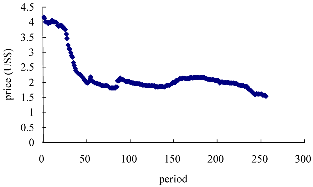
A real case is used to validate the effectiveness of the agent-based fuzzy collaborative intelligence approach. To this end, the price data of a DDR2 1G DRAM product have been collected for 256 days (see Figure 1).

Figure 1. The collected dynamic random access memory (DRAM) price data.

Figure 1. The collected dynamic random access memory (DRAM) price data.

Five existing approaches, moving average (MA), exponential smoothing (ES), BPN, ARIMA, and Chen’s fuzzy and neural approach, were also applied to this real case. Chen and Wang’s fuzzy interpolation approach was not compared because it is too subjective. MA uses a number of historical actual data values to generate a forecast. The moving period of MA has a reference value. Increasing the number of periods averaged does smooth out fluctuations better, but it makes the method less sensitive to real changes in the data. For this reason, this study tried a variety of moving periods (from 3 to 7), in which the best option was kept for later analyses.

ES is a weighted moving-average forecasting method, in which the latest estimate is equal to the old estimate adjusted by a fraction of the difference between the last period’s actual value and the old estimate. The smoothing constant in ES ranged from 0 to 1, and was optimized by enumerating some possible values

ARIMA is the generalization of an autoregressive moving average (ARMA) model that is usually used to fit time series data [35]. ARIMA consists of three stages: identification, estimation, and checking. To identify the order in the ARIMA process, the minimum information criterion (MINIC) method was employed. The stationarity and seasonal stationarity in the data were examined with the augmented dickey fuller (ADF) unit root tests [19].

BPN, also known as the multi-layer feed-forward neural network, is one of the most commonly used artificial neural networks. In BPN, inputs include the prices of K periods before. Here, K was set to be equal to the number of moving periods in MA for a fair comparison. The BPN was trained for 70,000 epochs per replication with randomized initial weights.

To evaluate the accuracy of each method, three measures including root mean squared error (RMSE), mean absolute error/deviation (MAE/D), and mean absolute percentage error (MAPE) were calculated. On the other hand, we assessed the precision of MA, ES, BPN, and ARIMA with 6σ:

$$6\mathrm{\sigma }=\mathrm{6}\sqrt{\frac{\sum _{\mathit{t}=\mathit{K}+\mathrm{1}}^{\mathit{T}}\mathrm{(}{\mathit{F}}_{\mathit{t}}-{\mathit{A}}_{\mathit{t}}\mathrm{)}{\mathrm{}}^{\mathrm{2}}}{\mathit{T}-\mathit{K}-\mathit{K}-\mathrm{1}}}$$

(56)

To the contrary, for evaluating the precision of Chen’s fuzzy and neural approach or the agent-based fuzzy collaborative intelligence approach, the average range of fuzzy price forecasts was considered. In both ways, the probability of containing the actual value in the fuzzy or interval forecast was approximately 100%. See Table 1 for the performances of various approaches in the two aspects. From the tabulated results it can be seen that the difference between the forecasting results and the real data is very small. The magnitude of the errors ranged from 0.00% to 3.47% with an average of only 0.59%. In fitting the collected data, the agent-based fuzzy collaborative intelligence approach achieved a very good performance. Among the three accuracy measures, MAPE and RMSE are similar in nature. The performance of the agent-based fuzzy collaborative intelligence approach with respect to these two measures was obviously better than those of the compared approaches. The advantage of the agent-based fuzzy collaborative intelligence approach in the accuracy aspect was most obvious when it came to MAE. MAE is highly indicative when the values are very small. We notice that ARIMA achieves good performance in this regard. The collaboration in the proposed methodology is aimed at the adjustment of the forecast by referencing the forecasts of others. The same treatment can be applied to ARIMA to further improve the forecasting performance of price forecasting. Meanwhile, the agent-based fuzzy collaborative intelligence approach elevated the forecasting precision to a level that was much higher than those of the five compared approaches. It became possible to establish a very narrow interval for every fuzzy price forecast, which is meaningful to many managerial purposes.

Table 1. The forecasting performances of different approaches.

		MA	ES	BPN	ARIMA	Chen’s approach	The proposed methodology
accuracy	MAE	0.040	0.020	0.052	0.016	0.015	0.013
	MAPE	1.72%	0.87%	2.47%	0.69%	0.64%	0.59%
	RMSE	0.068	0.040	0.077	0.030	0.028	0.024
precision	6σ or average range	0.313	0.238	0.468	0.182	0.105	0.079

Table 1. The forecasting performances of different approaches.

		MA	ES	BPN	ARIMA	Chen’s approach	The proposed methodology
accuracy	MAE	0.040	0.020	0.052	0.016	0.015	0.013
	MAPE	1.72%	0.87%	2.47%	0.69%	0.64%	0.59%
	RMSE	0.068	0.040	0.077	0.030	0.028	0.024
precision	6σ or average range	0.313	0.238	0.468	0.182	0.105	0.079

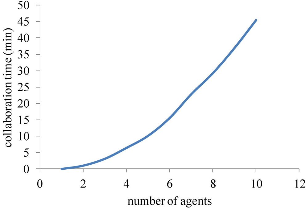
In the experiment, with the increase in the number of agents, the collaboration timesignificantly increased (see Figure 2).

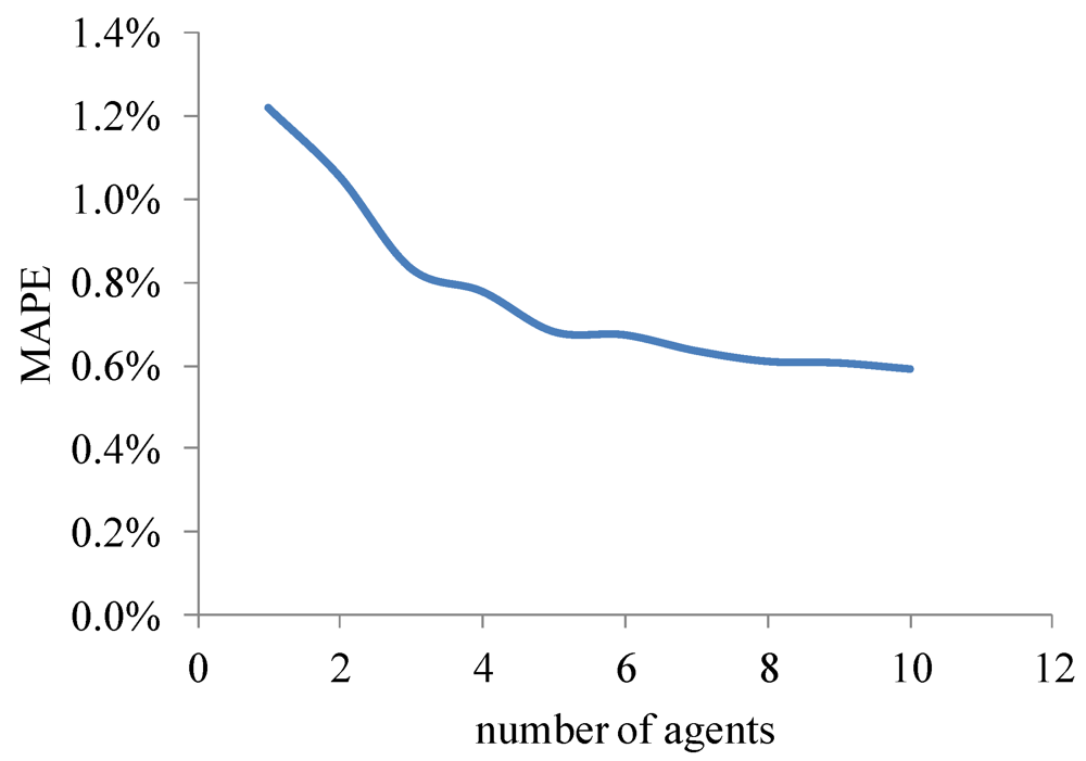
In contrast, the accuracy was improved with the increase in the number of agents (see Figure 3), but gradually approached to a constant value. Although it may appear that the agent-based fuzzy collaborative intelligence approach spent a considerable amount of time to improve the accuracy, but in fact only two agents and a handful of runs were required to achieve satisfactory results.

Figure 2. The required collaboration time.

Figure 2. The required collaboration time.

Figure 3. The accuracy of the agent-based fuzzy collaborative intelligence approach.

Figure 3. The accuracy of the agent-based fuzzy collaborative intelligence approach.

4. Conclusions

Much evidence has revealed that collaborative intelligence has potential application in forecasting. On the other hand, agent based collaboration has become an important field of research, and new applications of agent collaboration are expected to appear. In order to effectively predict the price of a DRAM product, an agent-based fuzzy collaborative intelligence approach is proposed in this study. In the agent-based fuzzy collaborative intelligence approach, each agent predicts the DRAM price using the FBPN approach based on its view. The agent then communicates its view and forecasting results to other agents with the aid of an automatic collaboration mechanism. After receiving that information, the agent modifies its setting and increases the overall accuracy. The forecasts by different agents are aggregated using an RBF.

After applying the agent-based fuzzy collaborative intelligence approach to a real case, the following experimental results were obtained:

(1) The aggregate results were considerably improved through the agents’ collaboration. Especially, the forecasting accuracy, measured in terms of MAE, MAPE, and RMSE, of the agent-based fuzzy collaborative intelligence approach was much better than those of some existing methods.

(2) It is therefore possible to predict the DRAM price level very precisely and accurately using a group of agents governed by an automatic collaboration mechanism.

More sophisticated collaboration mechanisms can be developed in similar ways in future studies. In addition, some advanced artificial neural networks have been proposed to improve the accuracy of time series prediction. These methods can be fuzzified to replace the FBPN used in this study. The proposed methodology can also be applied to predict other types of time series, such as stock price, production costs, product yield, etc. However, the computation becomes very complicated if many agents are involved. For this reason, future studies may restrict the size of the agent coalition.