Extracting Hierarchies from Data Clusters for Better Classification

1
Saint Petersburg State Polytechnical University, Polytechnicheskaya 29, Saint Petersburg 194064, Russia
2
HP Labs Russia, Artilleriyskaya 1, Saint Petersburg 191014, Russia
*
Authors to whom correspondence should be addressed.
Algorithms 2012, 5(4), 506-520; https://doi.org/10.3390/a5040506
Submission received: 2 July 2012
/
Revised: 24 September 2012
/
Accepted: 17 October 2012
/
Published: 23 October 2012
(This article belongs to the Special Issue Selected Papers from Text Mining Workshop at the 2012 SIAM International Conference on Data Mining)
Abstract
:In this paper we present the PHOCS-2 algorithm, which extracts a “Predicted Hierarchy Of ClassifierS”. The extracted hierarchy helps us to enhance performance of flat classification. Nodes in the hierarchy contain classifiers. Each intermediate node corresponds to a set of classes and each leaf node corresponds to a single class. In the PHOCS-2 we make estimation for each node and achieve more precise computation of false positives, true positives and false negatives. Stopping criteria are based on the results of the flat classification. The proposed algorithm is validated against nine datasets.
1. Introduction
The notion of classification is very general. It can be used in many applications, for example, text mining, multimedia processing, medical or biological sciences, etc. The goal of text classification is to assign an electronic document to one or more categories based on its contents.
The traditional single-label classification is concerned with a set of documents associated with a single label (class) from a set of disjoint labels. For multi-label classification, the problem arises as each document can have more than one label [1,2].
In some classification problems, labels are associated with a hierarchical structure, in which case the task belongs to hierarchical classification. If each document may correspond to more than one node of the hierarchy, then we deal with multi-label hierarchical classification. In this case, we can use both hierarchical and flat classification algorithms. In hierarchical classification, a hierarchy of classifiers can be built using a hierarchy of labels. If labels do not have a hierarchical structure, we can extract a hierarchy of labels from a dataset. It can help us to enhance classification performance.
However, there are some general issues in the area of hierarchical classification:
- In some cases classification performance cannot be enhanced using a hierarchy of labels. Some authors [3] showed that flat classification outperforms a hierarchical one in case of a large number of labels. So one should always compare a hierarchy with the flat case as a base line at each step of the hierarchy extraction.
- A hierarchy is built using some assumptions and estimations. One needs to make more accurate estimations in order not to let performance decrease due to rough computations. In hierarchical classification, a small mistake made by the top level of classifiers greatly affects the performance of the whole classification.
- Algorithms of extracting hierarchies require some external parameters. One needs to reach balance between the number of parameters and the effectiveness of an algorithm. Eventually, a smaller number of parameters leads to more simple usage.
In the previous work [4] we proposed and benchmarked the PHOCS algorithm that extracts a hierarchy of labels, and we showed that hierarchical classification could be better than a flat one. The main contribution of this work is enhancing the PHOCS algorithm.
We pursue the goal to increase performance of hierarchical classification using hierarchies built by the PHOCS algorithm. We want to reach this goal by solving the problems listed above. We make the estimation function more precise. We make estimation of false positives, true positives and false negatives and then calculate relative measures. We change stopping criteria as well. In the first version of the PHOCS, we used an external parameter that made the depth of our predicted hierarchy no more than five. We removed this parameter, and as stopping criteria, we now use a comparison of our estimated performance with the flat classification results.
2. State of the Art
In text classification, most of the studies deal with flat classification, when it is assumed that there are no relationships between the categories. There are two basic hierarchical classification methods, namely, the big-bang approach and the top-down level-based approach [5].
In the big-bang approach, a document is assigned to a class in one single step, whereas in the top-down level-based approach, classification is performed with the classifiers built at each level of a hierarchy.
In the top-down level-based approach, a classification problem is decomposed into a set of smaller problems corresponding to hierarchical splits in a tree. First, classes are distinguished at the top level, and then the lower level distinctions are determined only within the subclasses at the appropriate top-level class. Each of these sub-problems can be solved much more accurately as well [6,7]. Moreover, a greater accuracy is achievable because classifiers can identify and ignore commonalities between the subtopics of a specific class, and concentrate on those features that distinguish them [8]. This approach is used by most hierarchical classification methods due to its simplicity [5,6,9,10,11]. They utilize the known hierarchical (taxonomy) structure built by experts.
One of the obvious problems with the top-down approach is that misclassification at a higher level of a hierarchy may force a document to be wrongly routed before it gets classified at a lower level. Another problem is that sometimes there is no predefined hierarchy and one has first to build it. It is usually built from data or from data labels. We address the latter problem, which seems to us not that computationally complex, since the number of labels is usually less than the number of data attributes.
In our research, we follow the top-down level based approach utilizing a hierarchical topic structure to break down the problem of classification into a sequence of simpler problems.
There are approaches implying linear discriminant projection of categories to create hierarchies based on their similarities: [12,13]. They show that classification performance gets better as compared with a flat case. There is a range of methods aimed to reduce the complexity of training flat classifiers. Usually they partition data into two parts and create a two-level hierarchy, e.g., [14].
The HOMER method [15] constructs a Hierarchy Of Multi-label classifiERs, each one dealing with a much smaller set of labels with respect to and with a more balanced example distribution. This leads to an improved estimated performance along with linear training and logarithmic testing complexities with respect to . At the first step, the HOMER automatically organizes labels into a tree-shaped hierarchy. This is accomplished by recursively partitioning a set of labels into a number of nodes using the balance clustering algorithm. Then it builds one multi-label classifier at each node apart from the leaves.
In the PHOCS, we use the same concept of hierarchy and meta-labels. Tsoumakas et al. [16] also introduce the RAkEL classifier (RAndom k labELsets, k is a parameter specifying the size of labelsets) that outperforms some well-known multi-label classifiers.
In the recent work [17], the authors used datasets with predefined hierarchies and tried to guess them, but did not construct a hierarchy that could be good for classification. Generally, this is a more challenging task than a standard hierarchical multi-label classification, when classifiers are based on a known class hierarchy. In our research, we pursue a similar objective.
In 2011 the second Pascal challenge on large-scale classification was held. Wang et al. [3] got the first place in two of the three benchmarks. They enhanced the flat kNN method and outperformed hierarchical classification. They used an interesting method of building a hierarchy as well, which employs only existing labels without the use of any meta-labels. The performance was lower than in the flat case. There are two specific issues when building a taxonomy in a such way. For example, Reuters-21578 already has meta-labels that generalize other labels. They are not used in the classification. Some datasets do not have such meta-labels or any structure of labels. Another issue is that two very similar labels, associated with two contiguous categories, should be on one layer. However, in such way of building hierarchy the may be put in a parent-child relation. To solve the mentioned issues, we will build a hierarchy using meta-labels.
3. Multi-Label Hierarchical Classification
3.1. General Concept
The main idea is transformation of a multi-label classification task with a large set of labels L into a tree-shaped hierarchy of simpler multi-label classification tasks, each one dealing with a small number k of labels: (sometimes . Below follows the explanation of the general concept of the multi-label hierarchical classification [4].
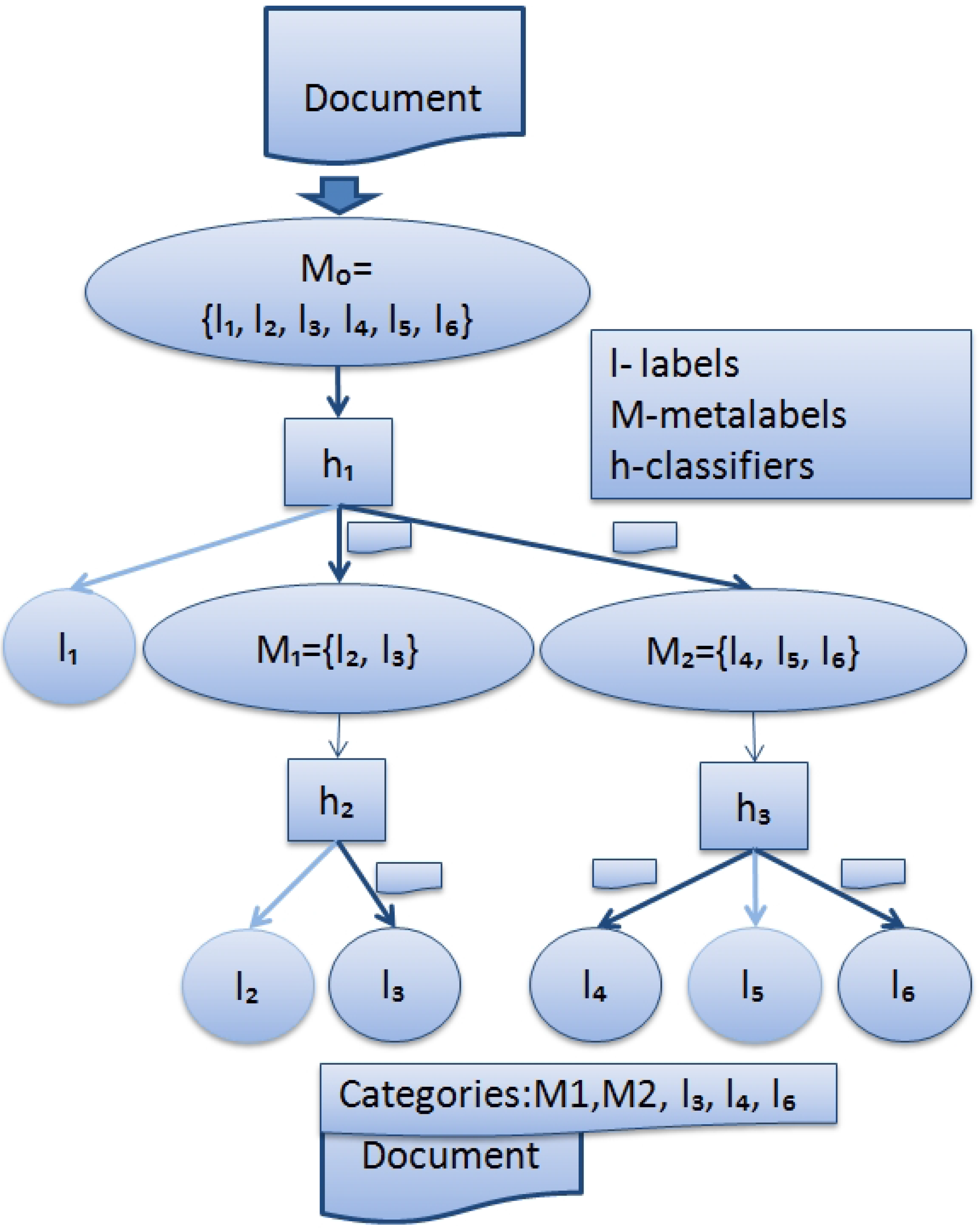
Each node n of this tree contains a set of labels . Figure 1 shows 6 leaves and 3 internal nodes. There are leaves, each containing a singleton (a single element set) with a different label j of L. Each internal node n contains a union of labelsets of its children: . The root accommodates all the labels: .
Meta-label of node n is defined as conjunction of the labels associated with that node: . Meta-labels have the following semantics: a document is considered annotated with the meta-label if it is annotated with at least one of the labels in . Each internal node n of a hierarchy also accommodates a multi-label classifier . The task of is to predict one or more meta-labels of its children. Therefore, the set of labels for is .
Figure 1 shows a sample hierarchy produced for a multi-label classification task with 6 labels.
Figure 1.
Hierarchical multi-label classification work flow.

For multi-label classification of a new document, the classifier starts with and then forwards it to the multi-label classifier of the child node c only if is among the predictions of . The main issue in building hierarchies is how to distribute the labels of among the k children. One can distribute k subsets in such a way that the labels belonging to the same subset remain similar. In [15], the number k of labels is a set given for each .
3.2. Building One Layer: Example
In this work, we solve the problem of distribution of labels among children nodes by choosing the best value of k at each node according to the estimation of the hierarchy performance. We use the divide-and-conquer paradigm for our algorithm design [15]. Our algorithm starts from the whole set of labels and its goal is to build a hierarchy of labels optimizing classification performance. In each step, we divide the current set of labels into groups that correspond to the child nodes of that set. Our algorithm is recursive and proceeds until the current set contains only one label. Such sets will be leaves of the hierarchy.
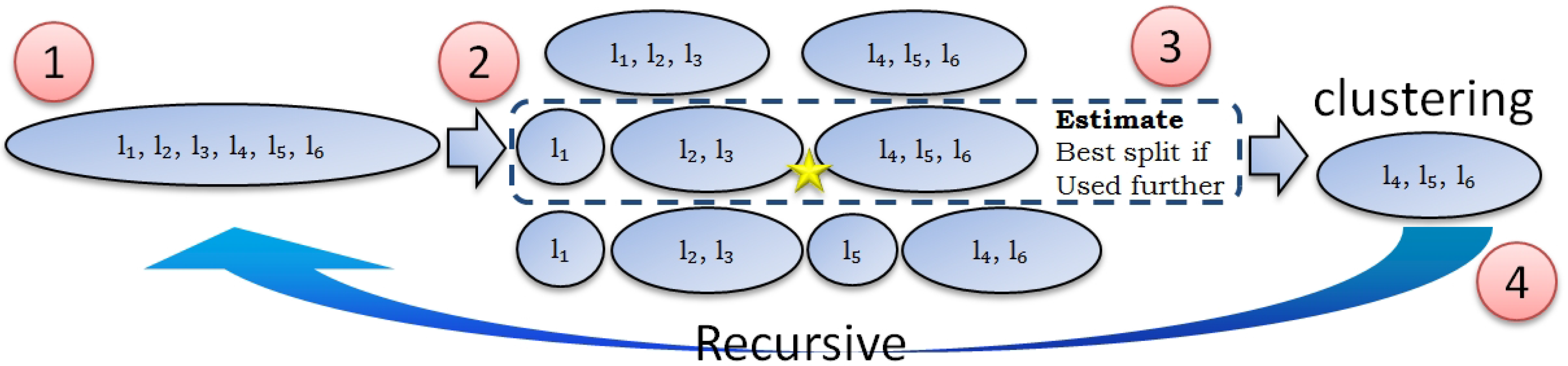
Illustration of one step of our algorithm can be found in Figure 2. It will proceed in the following way.
Figure 2.
Example: building one layer.

- We have 6 labels.
- We cluster labels with different k, which results in 3 different partitions ().
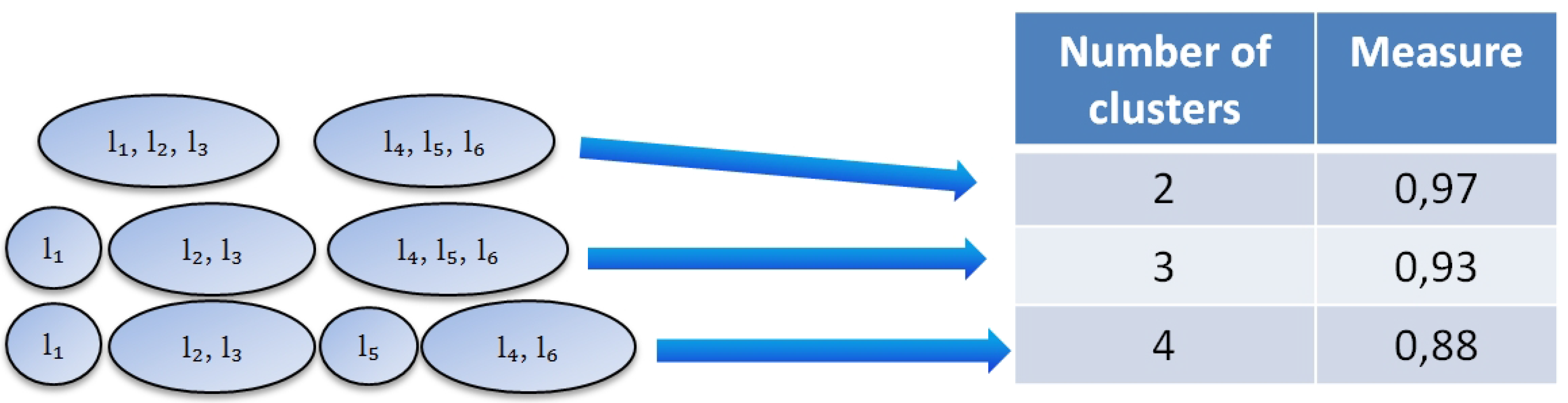
- We estimate which partition is the best for the classification using the performance estimation function (chapter 4). In this example we use partition number 2 (Figure 3).
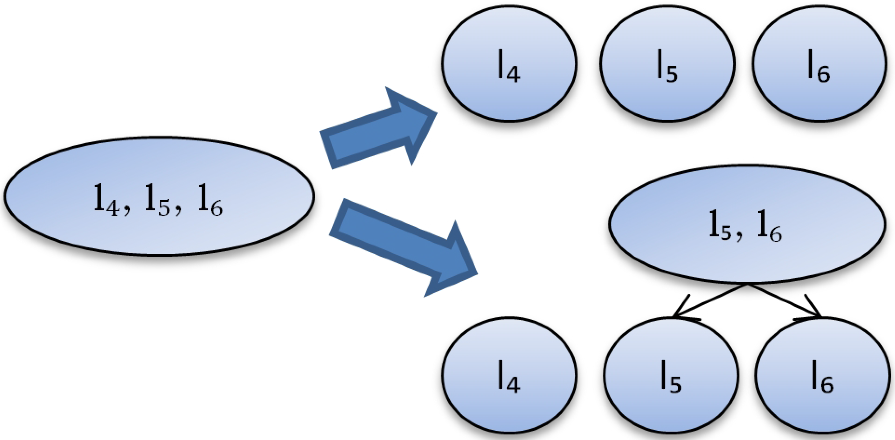
- We use the partition selected at the previous step and go to step 2 to process {} (Figure 4). There is no need to make clustering for {} and {} since their partitioning is obvious.
Figure 3.
Example of partitions.
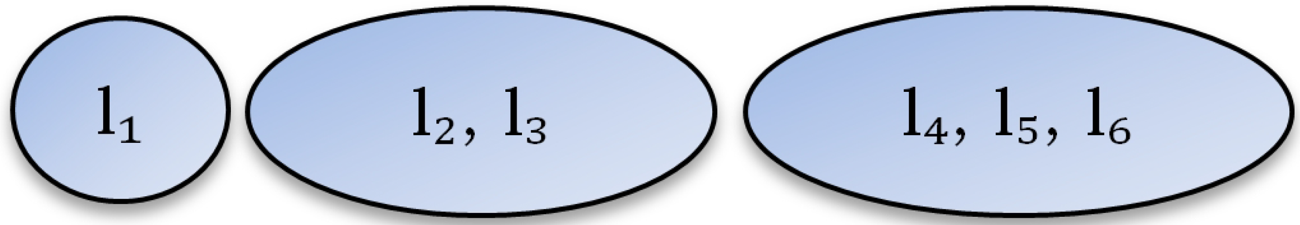
Figure 4.
Different ways of splitting the labels.

3.3. Algorithm For Building Hierarchies
Our algorithm is recursive (Algorithm 1). It takes a training dataset as an input, and the minimum and maximum numbers of clusters and . It starts from the whole set of labels, makes K-means clustering of them for a different number of clusters from to (line 4). We cluster labels using documents as binary features for clustering. If a label is associated with a document, then a corresponding feature value is 1, otherwise 0. Feature space size equals N, where N is the number of documents. We compose meta-labels from clusters for each partition (line 5) and measure their efficiency using a classification task (line 6).
All sets of clusters are candidates for the next layer of the hierarchy. We choose the best partition with the help of an estimation algorithm (line 8). Using the best-estimated partition, we build meta-labels (each meta-label consists of classes from one cluster, line 10). After that, we make this process recursive for the child meta-labels.
3.4. Algorithm Complexity
Let equals 2. Denote N as the number of documents. Denote M as the number of attributes. Denote as the number of labels. Consider the computational complexity of the first step of the algorithm. Each clustering has complexity (Algorithm 1). We will also train binary classifiers for one clustering (line 6 in Algorithm 1), the complexity of training one classifier is . So the complexity of cycle (lines 3–7 in Algorithm 1) has complexity . The prediction function has the complexity for each cluster. For all the clusters it is (line 8 in Algorithm 1). So the running time in the root node can be defined as the sum of these quantities: .
| Algorithm 1 The PHOCS algorithm for hierarchy building | |
| 1: | function Hierarchy() |
| 2: | |
| 3: | for do |
| 4: | |
| 5: | |
| 6: | |
| 7: | end for |
| 8: | |
| 9: | if then |
| 10: | |
| 11: | for do |
| 12: | |
| 13: | |
| 14: | end for |
| 15: | end if |
| 16: | end function |
| 17: | function PerformanceMeasure() |
| 18: | |
| 19: | return |
| 20: | end function |
| 21: | function PerfEstimate() |
| 22: | //Described in Section 4 |
| 23: | end function |
Let us consider the computational complexity of building one layer. Suppose each node at this level has N documents, although they are fewer. Since each label of L lies in a single cluster, the total complexity of all clusterings on the layer is . Similarly, the complexity of the prediction function for all clusters in all nodes will not exceed . Denote the mean number of labels in the document as A, whereas in fact, the number of documents in all nodes at the same level does not exceed . If the classifier learning algorithm has linear complexity with respect to the number of documents, the complexity of building all classifiers will not exceed . So the running time of building a layer can be defined as the sum of these quantities: . In most cases it is less than , where is complexity of building a multi-label classifier in binary transformation case.
We showed the complexity of building one layer. The number of layers in a good hierarchy does not exceed 5. In our paper we used the decision tree algorithm [18]. For .
4. Performance Estimation
4.1. General Idea
The goal of the performance estimation function is to estimate classification performance of each partition. With our estimation function, we want to determine which partition is better. We employ a training set for this function. At the same time we need a test set in order to decide which partition is better. We use a part of the training set for this, and the other part remains for training purposes.
We build a classifier for each partition. Each cluster represents one class. We classify the documents and get the performance measure that shows how good a particular partition is. Various measures can be used in our algorithm. The goal of our algorithm is to build a hierarchy with an optimum performance measure. For example, for partition into 2 clusters we get the classification performance measure (Figure 5). For partition into 3 clusters the measure is and for partition into 4 clusters it is .
Figure 5.
Example: filling in the table.

We believe that on further layers of the hierarchy, the partition into k clusters will be the same as in the performance table (Figure 5). We also know various features of clusters, such as size, diversity, etc. Therefore, it is possible to explore all possible partitions as well as final hierarchies and to estimate their performance. For example, one may want to make estimation for partition into 3 clusters (Figure 3).
Cluster {} has only one class and we assume that its performance is 1. Cluster {} has 2 classes and its performance is believed to be similar to the performance from the table, which is . Cluster {} can be clustered further in 2 different ways (Figure 4). We calculate the number of labels at different levels for the sake of simplicity. So we do not distinguish which labels are in the cluster of size 2: {}, {} or {}. Finally, we have only two different partitions (Figure 4).
We make performance estimation for the first partition based on the table from Figure 5. It is . The performance of the second partition cannot be estimated using the referenced table since it contains a sub-hierarchy. We propose a certain approach for doing this.
4.2. Approach
In the previous version of our algorithm (we will refer to it as to PHOCS-1) we made estimation in the following way. We used -measure as a performance measure and assumed that the -measure becomes smaller layer by layer (as the hierarchy is growing), that is, the -measure on layer k is larger than on layer . We estimated it at level as , where i is the layer number. This estimation is rather rough and it is possible to make it finer. We propose to use absolute values of errors and the structure of nodes as well as more information about clusters—their size and performance values.
We will denote:
- C – cluster size;
- – the number of documents in the cluster;
- K – the number of child clusters;
- – the average number of labels for documents in the cluster;
- S – the number of possible further partitions for the cluster;
- index is used for estimated numbers and measures;
- index is used for the best estimation for the cluster (among all possible partitions of this cluster);
- index is used for estimation of the whole partition (split);
- index denotes the number of partitions for a particular cluster;
- index is used for the values of the performance measure in the table that we fill in (like in Figure 5). Each record in the table corresponds to a specific number of child clusters K.
Our goal is to estimate the absolute values of true positives (), false negatives () and false positives (). Then we have to calculate relative performance measures that can be used for optimizing the hierarchy, such as -measure (), Precision () or Recall ().
Figure 6.
Estimating performance for cluster {}.
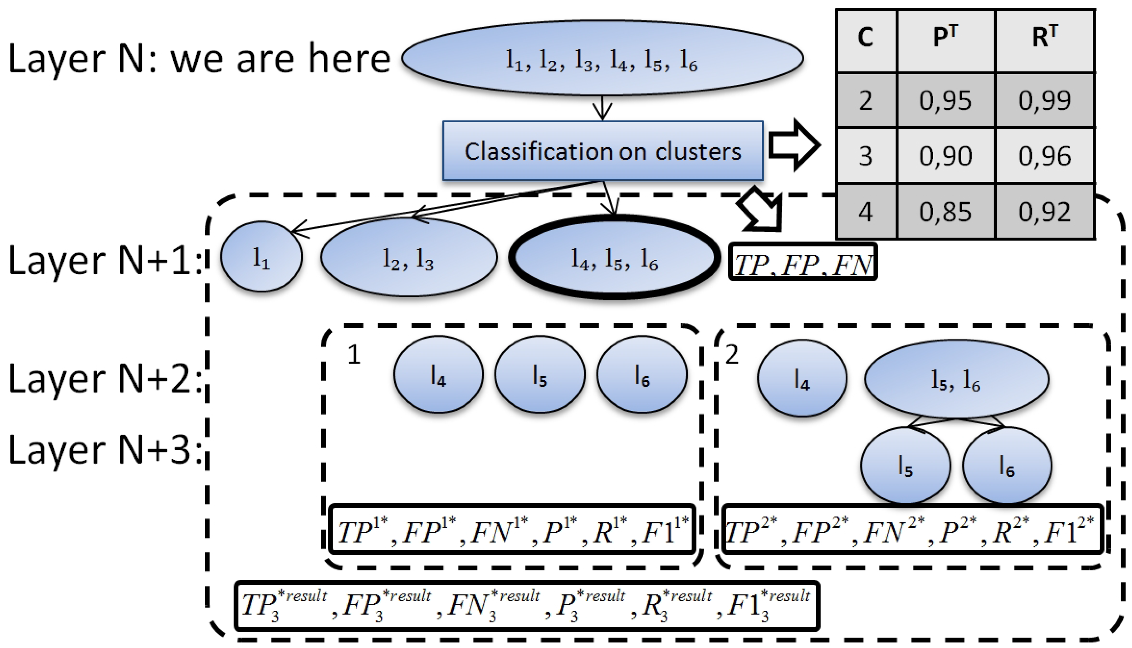
The example of estimation process is represented in Figure 6. Assume that we are currently on layer N. On this layer we have already made clustering (Figure 2, step 2) and filled in the performance table (Figure 5). Assume, we are estimating classification performance for one of the partitions {} (Figure 3 and Figure 6) with two ways of splitting (Figure 4, ). , , and are computed in the following way:
- . The number of true positives will decrease with each next level of the hierarchy. will depend on R and we will approximate it with the following function: . K equals 3 for and 2 for (Figure 6, layer ).
- . We know , , . So, .
- . The main problem is to estimate . Indeed the result of should be between and . We use a rather pessimistic estimation of it: .
We computed , , on different layers of our cluster. We believe that a hierarchy should be rather balanced with leaves on the last two layers only. Let us denote the last layer as M. Then there are two groups of leaves: leaves on the last layer () and leaves on the previous layer (). . For example, Figure 6 represents a cluster of size 3. All leaves are on layer for the first split. One leaf is on layer and two leaves are on layer for the second split.
Then we are able to compute relative measures for our cluster:
Therefore, we are able to find the best further partitioning of the cluster. If we maximize , then the best partitioning of the cluster will be partitioning with the maximal . We will use with absolute estimations for the best estimated partitioning of our cluster. .
We take into account the size of clusters in order to compute estimation for the whole partition (split). The more documents there are in a cluster the higher influence they have on the estimation. Estimation is made for each cluster separately. First, we find the best further partitioning of the cluster. Second, we summarize the absolute numbers:
Now we are able to compute the relative measures ,, and .
The general idea is to minimize the number of external parameters in our algorithm. should always equal 2, and is the only external parameter and it should not be greater than the square root of . We have changed the stopping criteria of our algorithm. We make comparison with the flat classification result as stopping criteria. If our prediction is worse than the flat case, then we stop further building of the hierarchy (in the previous version we stopped building a hierarchy after several layers).
4.3. Performance Estimation Function
Let us summarize the proposed approach for performance estimation in a sequence of steps. We had completed the following steps before the call of the performance estimation function:
- A certain number of labels is given.
- The labels are clustered. As a result, we have different partitions.
- Classification is done using the clusters for different partitions.
- A table with the performance measures of classification for all clusters is filled in (, and ). , , for all clusters are saved.
The input for the performance estimation function is the following:
- Partitions configuration (the number of different partitions, their sizes).
- Clusters configuration (, , as the result of classification, C, , ).
- A table with the measures (, and ).
Finally, we are able to list all steps of the performance estimation function (denoted as function PerfEstimate in the Algorithm 1):
- For each possible further partitioning of each cluster in each partition:
- (a)
- count the number of leaves on different layers of the predicted taxonomy (, )
- (b)
- estimate the number of positives and negatives , , .
- (c)
- estimate relative measures , , .
- For each cluster, estimate the best further partitioning ().
- For each partition (for each k), estimate the absolute and relative parameters on the current layer: , , , , , .
- Choose the best partition based on .
The estimation function returns the best partition and the estimated performance for it.
5. Experiments
All the experiments are performed on multi-label datasets available at [19]. Table 1 exhibits basic statistics, such as the number of examples and labels, along with the statistics that are relevant to the label sets [16].
Multi-Label classification problem can be solved in different ways [2]. Problem transformation methods allow converting a multi-label problem to a single-label one. Below is the list of the most frequently used approaches:
- Binary Relevance. One builds a classifier for each label, which will make a decision about this label.
- Label Power-set transformation. One builds a multiclass classifier, where each class corresponds to a set of labels associated with a document.
- One vs. one. One trains a classifier for each pair of labels. The decision is made by voting.

| Name | Docs | Labels | Bound of labelsets | Actual labelsets |
|---|---|---|---|---|
| Mediamill | 43907 | 101 | 43907 | 6555 |
| Bibtex | 7395 | 159 | 7395 | 2856 |
| Medical | 978 | 45 | 978 | 94 |
| Enron | 1702 | 53 | 1702 | 753 |
| Yeast | 2417 | 14 | 2417 | 198 |
| Genbase | 662 | 27 | 662 | 32 |
| Corel5k | 5000 | 374 | 5000 | 3175 |
| CAL500 | 502 | 174 | 502 | 502 |
| Scene | 2407 | 6 | 64 | 15 |
We use Binary Relevance transformation because of the nature of the data (Table 1). The last column shows the number of classes in case of Label Power-set transformation. This transformation can work on Scene, Genbase and Medical. In other datasets, the number of classes will be rather large so the number of training examples for each class will be low and classification performance will be poor as well.
It is also rather hard to build one versus one flat classifier. There will be classifiers for Corel5k. It is much easier to use it in a hierarchy, and we plan to do it in our future work.
Each dataset is divided into the training and test parts in the proportion 2 to 1, respectively. There are no any other transformations of the datasets. In particular, there is no attribute selection. The first four datasets are used in all experiments and the last five are used only with the PHOCS-2.
The decision tree algorithm [18] is chosen as the basic multi-label classifier. The K-means algorithm is used for clustering and building hierarchies. The micro and macro measures of classification accuracy (precision (P), recall (R) and -measure) are used [20].
The parameter values for the PHOCS are chosen as and . Such is chosen since the number of labels in our experiments has the order of 100, so the hierarchy contains at least 2 layers.
The experiment results are represented in Table 2.
We removed the external parameter, so the PHOCS-2 has only two parameters: , which should always equal 2, and , which can be the only external parameter in the ideal case. We got a better -measure in comparison with the results from [4] for all four datasets that we used there. In all cases the current version of the algorithm demonstrated the best performance (-measure).
The experimental study of the PHOCS-2 performance on nine multi-label datasets justifies its effectiveness. We got significantly better results in five of them compared with the flat case. It was difficult to improve the result of the Genbase, because its performance is already , and we have not improved the performance in the Mediamill and the Yeast. HOMER [15] was tested only on two datasets. One of them is Mediamill and we can compare results. There is no baseline in [15]. PHOCSv2 outperforms HOMER by in -measure on Mediamill dataset.
| Dataset name | Classifier topology | MICRO | MACRO | ||||
|---|---|---|---|---|---|---|---|
| F1 | P | R | F1 | P | R | ||
| Mediamill | Flat | 0.54 | 0.66 | 0.45 | 0.10 | 0.24 | 0.08 |
| PHOCS v1 | 0.53 | 0.58 | 0.52 | 0.13 | 0.24 | 0.14 | |
| PHOCS v2 | 0.53 | 0.55 | 0.52 | 0.11 | 0.22 | 0.10 | |
| Bibtex | Flat | 0.31 | 0.81 | 0.19 | 0.14 | 0.40 | 0.11 |
| PHOCS v1 | 0.37 | 0.61 | 0.21 | 0.22 | 0.38 | 0.18 | |
| PHOCS v2 | 0.39 | 0.65 | 0.28 | 0.22 | 0.44 | 0.18 | |
| Medical | Flat | 0.80 | 0.85 | 0.75 | 0.26 | 0.32 | 0.25 |
| PHOCS v1 | 0.82 | 0.84 | 0.81 | 0.30 | 0.34 | 0.30 | |
| PHOCS v2 | 0.83 | 0.86 | 0.79 | 0.30 | 0.34 | 0.30 | |
| Enron | Flat | 0.46 | 0.66 | 0.35 | 0.09 | 0.13 | 0.08 |
| PHOCS v1 | 0.50 | 0.62 | 0.42 | 0.10 | 0.15 | 0.09 | |
| PHOCS v2 | 0.50 | 0.55 | 0.46 | 0.11 | 0.15 | 0.11 | |
| Yeast | Flat | 0.59 | 0.61 | 0.58 | 0.38 | 0.41 | 0.38 |
| PHOCS v2 | 0.59 | 0.59 | 0.60 | 0.39 | 0.39 | 0.39 | |
| Genbase | Flat | 0.97 | 1.00 | 0.95 | 0.67 | 0.70 | 0.65 |
| PHOCS v2 | 0.98 | 1.00 | 0.96 | 0.68 | 0.70 | 0.67 | |
| Corel5k | Flat | 0.04 | 0.24 | 0.02 | 0.00 | 0.01 | 0.00 |
| PHOCS v2 | 0.09 | 0.18 | 0.06 | 0.01 | 0.01 | 0.00 | |
| CAL500 | Flat | 0.37 | 0.50 | 0.30 | 0.10 | 0.13 | 0.10 |
| PHOCS v2 | 0.40 | 0.37 | 0.43 | 0.16 | 0.16 | 0.20 | |
| Scene | Flat | 0.61 | 0.67 | 0.57 | 0.52 | 0.61 | 0.50 |
| PHOCS v2 | 0.63 | 0.66 | 0.59 | 0.54 | 0.61 | 0.54 | |
In most cases, our algorithm provides better F1 due to better Recall. We are able to optimize other measures as well. It is useful when one has specific requirements to a classifiers performance.
6. Results and Conclusion
We proposed several enhancements for the PHOCS algorithm that builds hierarchies from flat clusterings in order to enhance classification accuracy. To build a better hierarchy we used absolute values of errors, employed the number and structure of nodes, cluster sizes and individual performance values for each cluster. We changed the stopping criteria as well to compare our hierarchy with a flat one.
The experimental study shows effectiveness of the enhancements. We have removed one of the parameters as well. As a result, it has become easier to use the PHOCS.
Our future work will be related to improving the performance estimation function and adding a possibility to return to a previous layer in case of false prediction. We would like to use or create a classifier that can take advantage of a hierarchy. Another goal is to compare our algorithm with EkNN [3] that has won the second Pascal challenge.
References
- Xue, G.R.; Xing, D.; Yang, Q.; Yu, Y. Deep classification in large-scale text hierarchies. In Proceedings of the 31st Annual International ACM SIGIR Conference on Research and Development in Information Retrieval, Singapore, Singapore, 20–24 July 2008; ACM: New York, NY, USA, 2008; pp. 619–626. [Google Scholar]
- Tsoumakas, G.; Katakis, I. Multi-Label classification: An overview. Int. J. Data Warehous. Min. 2007, 3, 1–13. [Google Scholar] [CrossRef]
- Wang, X.; Zhao, H.; Lu, B.L. Enhanced K-nearest neighbour algorithm for largescale hierarchical Multi-label Classification. In Proceedings of the Joint ECML/PKDD PASCAL Workshop on Large-Scale Hierarchical Classification, Athens, Greece, 5 September 2011.
- Ulanov, A.; Sapozhnikov, G.; Shevlyakov, G.; Lyubomishchenko, N. Enhancing accuracy of multilabel classification by extracting hierarchies from flat clusterings. In Proceedings of the 2011 22nd International Workshop on Database and Expert Systems, Toulouse, France, 29 August–2 September 2011; pp. 203–207.
- Sun, A.; Lim, E.P. Hierarchical text classification and evaluation. In ICDM ’01: Proceedings of the 2001 IEEE International Conference on Data Mining, San Jose, CA, USA, 29 November–2 December 2001; pp. 521–528.
- Dumais, S.; Chen, H. Hierarchical classification of web content. In Proceedings of the 23rd Annual International ACM SIGIR Conference On Research and Development in Information Retrieval, Athens, Greece, 24–28 July 2000; ACM: Athens, Greece, 2000; pp. 256–263. [Google Scholar]
- Pulijala, A.; Gauch, S. Hierachcal text classification. In Proceedings of the CITSA 2004, Orlando, FL, USA, 18–21 July 2004; pp. 257–262.
- D’Alessio, S.; Murray, K.; Schiaffino, R.; Kershenbaum, A. The effect of using hierarchical classifiers in text categorization. In Proceedings of 6th International Conference Recherche dInformation Assistee par Ordinateur (RIAO-00), Paris, France, 12–14 April 2000; pp. 302–313.
- Koller, D.; Sahami, M. Hierarchically classifying documents using very few words. In Proceedings of ICML-97, 14th International Conference on Machine Learning, Nashville, TN, USA, 8–12 July 1997; Fisher, D.H., Ed.; Morgan Kaufmann Publishers: San Francisco, CA, USA, 1997; pp. 170–178. [Google Scholar]
- Chakrabarti, S.; Dom, B.; Indyk, P. Enhanced hypertext categorization using hyperlinks. In SIGMOD ’98: Proceedings of the 1998 ACM SIGMOD International Conference on Management of Data, Seattle, WA, USA, 2–4 June 1998; ACM Press: New York, NY, USA, 1998; Volume 27, pp. 307–318. [Google Scholar]
- Weigend, A.S.; Wiener, E.D.; Pedersen, J.O. Exploiting hierarchy in text categorization. Inf. Retr. 1999, 1, 193–216. [Google Scholar] [CrossRef]
- Gao, B.; Liu, T.Y.; Feng, G.; Qin, T.; Cheng, Q.S.; Ma, W.Y. Hierarchical taxonomy preparation for text categorization using consistent bipartite spectral graph copartitioning. IEEE Trans. Knowl. Data Eng. 2005, 17, 1263–1273. [Google Scholar]
- Li, T.; Zhu, S.; Ogihara, M. Hierarchical document classification using automatically generated hierarchy. J. Intell. Inf. Syst. 2007, 29, 211–230. [Google Scholar] [CrossRef]
- Cesa-Bianchi, N.; Gentile, C.; Zaniboni, L. Hierarchical classification: Combining bayes with SVM. In ICML ’06: Proceedings of the 23rd International Conference on Machine Learning, Pittsburg, PA, USA, 25–29 June 2006; ACM: New York, NY, USA, 2006; pp. 177–184. [Google Scholar]
- Tsoumakas, G.; Katakis, I.; Vlahavas, I. Effective and efficient multilabel classification in domains with large number of labels. In Proceedings of the ECML/PKDD 2008 Workshop on Mining Multidimensional Data (MMD’08), Antwerp, Belgium, 15–19 September 2008.
- Tsoumakas, G.; Katakis, I.; Vlahavas, I. Random k-labelsets for multilabel classification. Knowl. Data Eng. IEEE Trans. 2011, 23, 1079–1089. [Google Scholar] [CrossRef]
- Brucker, F.; Benites, F.; Sapozhnikova, E. Multi-Label classification and extracting predicted class hierarchies. Pattern Recognit. 2011, 44, 724–738. [Google Scholar] [CrossRef]
- Webb, G.I. Decision tree grafting from the all-tests-but-one partition. In Proceedings of the 16th International Joint Conference on Artificial Intelligence-Volume 2, Stockholm, Sweden, 31 July–6 August 1999; Morgan Kaufmann Publishers Inc.: San Francisco, CA, USA, 1999; pp. 702–707. [Google Scholar]
- Machine Learning & Knowledge Discovery Group Home Page. Available online: http://mlkd.csd.auth.gr/multilabel.html (accessed on 22 October 2012).
- Manning, C.D.; Raghavan, P.; Schutze, H. Introduction to Information Retrieval; Cambridge University Press: New York, NY, USA, 2008. [Google Scholar]
© 2012 by the authors; licensee MDPI, Basel, Switzerland. This article is an open access article distributed under the terms and conditions of the Creative Commons Attribution license (http://creativecommons.org/licenses/by/3.0/).
Share and Cite
MDPI and ACS Style
Sapozhnikov, G.; Ulanov, A. Extracting Hierarchies from Data Clusters for Better Classification. Algorithms 2012, 5, 506-520. https://doi.org/10.3390/a5040506
AMA Style
Sapozhnikov G, Ulanov A. Extracting Hierarchies from Data Clusters for Better Classification. Algorithms. 2012; 5(4):506-520. https://doi.org/10.3390/a5040506
Chicago/Turabian StyleSapozhnikov, German, and Alexander Ulanov. 2012. "Extracting Hierarchies from Data Clusters for Better Classification" Algorithms 5, no. 4: 506-520. https://doi.org/10.3390/a5040506