Finite Element Quadrature of Regularized Discontinuous and Singular Level Set Functions in 3D Problems

Abstract

Regularized Heaviside and Dirac delta function are used in several fields of computational physics and mechanics. Hence the issue of the quadrature of integrals of discontinuous and singular functions arises. In order to avoid ad-hoc quadrature procedures, regularization of the discontinuous and the singular fields is often carried out. In particular, weight functions of the signed distance with respect to the discontinuity interface are exploited. Tornberg and Engquist (Journal of Scientific Computing, 2003, 19: 527–552) proved that the use of compact support weight function is not suitable because it leads to errors that do not vanish for decreasing mesh size. They proposed the adoption of non-compact support weight functions. In the present contribution, the relationship between the Fourier transform of the weight functions and the accuracy of the regularization procedure is exploited. The proposed regularized approach was implemented in the eXtended Finite Element Method. As a three-dimensional example, we study a slender solid characterized by an inclined interface across which the displacement is discontinuous. The accuracy is evaluated for varying position of the discontinuity interfaces with respect to the underlying mesh. A procedure for the choice of the regularization parameters is proposed.

1. Introduction

Regularization of singular and highly localized fields is a widely diffuse practice in several computational mechanics fields, such as thermal analysis, advection-diffusion problems [1], in Boundary Element Method applications [2], electronic structure calculations [3], for applications to modeling delamination in multilayered composites [4], and for capturing the behaviour of plastic hinges in Timoshenko beam elements [5]. Among other methods [6,7], the eXtended Finite Element Method (XFEM) [6,8,9,10] is a powerful technique for modelling engineering problems characterized by discontinuous and singular functions. XFEM is based on incorporating Heaviside and highly localized functions reproducing the expected shape of the interpolated fields. In this context, quadrature of terms containing discontinuous and singular functions is performed by subdividing the elements crossed by discontinuities in quadrature sub-domains [8], or, alternatively, by making use of adaptive quadrature [3,11]. Subdivision into quadrature sub-domains can be cumbersome in the multidimensional case. Ventura [12] proposed an alternative technique for the integration of discontinuous integrands based on the use of equivalent polynomials.

Alternatively, regularization makes it possible to use standard Gauß quadrature and to avoid sub-domain quadrature. Regularized XFEM is also an effective alternative to nonlocal and cohesive crack-models [13,14,15,16]. The key concept underlying regularization of discontinuous and highly localized functions is simple: the Dirac delta function is replaced by a weight function whose support is governed by a length parameter ρ, while the standard Heaviside function is constructed by integration of such a weight function. For vanishing ρ, the Heaviside and delta functions are recovered [17]. Regularization obviously introduces approximations in the computation. Tornberg et al. [18,19] proved that the total error of integration can be split into the sum of the analytical and the numerical (quadrature) error. Specifically, the analytical error is governed by the approximation of the delta function, while the numerical error is governed by the differentiability of the regularized delta function besides the order of the quadrature rule.

The level set method [20] is a highly successful computational technique for tracking the spatial evolution of three-dimensional interfaces. An attractive feature is that interfaces are implicitly described and do not need to be parameterized. The use of the level set method [20] leads to a straightforward extension of regularized Heaviside and delta functions to the multidimensional case. Albeit regularization can be carried out by means of compact support weight functions, in [1,3,19,21] it has been proved that three-dimensional extensions based on compact support weight functions can lead to inconsistent results, as errors do not reduce with discretization refinement. The problem is that the moment conditions no longer hold for any shift (dilation) of the weight function with respect to the quadrature grid. Hence non-compact support weight functions should be used.

The structure of the paper is briefly summarized. In Section 2, we define a displacement field discontinuous across an interface. The discontinuity is expressed by means of the Heaviside function. The strain obtained by differentiation displays a delta function dependence, i.e., it is singular. The necessity of numerically integrating these functions arises. In order to perform quadrature in a more straightforward way, we replace the delta function with a regularized version. Regularization is achieved by introducing a smooth weight function whose support is governed by a regularization length (Section 3). Following [22], we exploit the relationship between Fourier transforms of the weight functions and accuracy of the regularization procedure in Section 3.1. As compact support functions were shown to be non-satisfying, we introduce non-compact support weight functions in Section 3.3. The truncation error is discussed in Section 3.2. Section 4 contains a brief presentation of the regularization procedure based on XFEM. A three-dimensional bar characterized by a discontinuous interface is discussed as a benchmark test in Section 5. In particular, the case of inclined discontinuities with respect to the underlying mesh is shown to be sensitive to the truncated support width. The influence of the truncation of the non-compact support is illustrated. A procedure for choosing the regularization parameter and the truncated support width is proposed.

2. Regularization in the Level Set Context

Let the volume V be divided into $V_1$ and $V_2$ by the interface Γ. At any point $\mathbf{x}\in \Gamma$, the interface is characterized by the normal vector $\mathbf{n}\left(\mathbf{x}\right)$. The position of Γ is implicitly defined by means of the signed distance function with respect to Γ [20]

$$d\left(\mathbf{x}\right)=\left\{\begin{array}{cc}\text{dist}(\mathbf{x},\Gamma )\hfill & \text{if}\mathbf{x}\in V_1\hfill \\ -\text{dist}(\mathbf{x},\Gamma )\hfill & \text{if}\mathbf{x}\in V_2\hfill \end{array}\right.$$

(1)

We introduce the Heaviside function $\mathscr{H}\left(d\right(\mathbf{x}\left)\right)$ such that $\mathscr{H}\left(d\right(\mathbf{x}\left)\right)=1$ for $d\left(\mathbf{x}\right)>0$ and $\mathscr{H}\left(d\right(\mathbf{x}\left)\right)=-1$ for $d\left(\mathbf{x}\right)\le 0$, and focus on discontinuous functions of the type

$$\mathbf{u}\left(\mathbf{x}\right)=\mathbf{v}\left(\mathbf{x}\right)+\mathscr{H}\left(d\right(\mathbf{x}\left)\right)\mathbf{j}\left(\mathbf{x}\right)$$

(2)

where $\mathbf{v}\left(\mathbf{x}\right)$ is the regular part of the field u, while $\mathbf{j}\left(\mathbf{x}\right)$ denotes the amplitude of the jump of $\mathbf{u}\left(\mathbf{x}\right)$ across Γ. Differentiation of the discontinuous vector function (2) leads to a singular function of the type

$$\epsilon \left(\mathbf{x}\right)=\nabla \mathbf{u}\left(\mathbf{x}\right)=\nabla \mathbf{v}\left(\mathbf{x}\right)+\mathscr{H}\left(\mathbf{x}\right)\nabla \mathbf{j}\left(\mathbf{x}\right)+\delta \left(d\right(\mathbf{x}\left)\right)\left(\mathbf{j}\right(\mathbf{x})\otimes \mathbf{n}(\mathbf{x}\left)\right)$$

(3)

where ∇ denotes differentiation. The delta function $\delta \left(d\right(\mathbf{x}\left)\right)$ is introduced through the generalized gradient $\nabla \mathscr{H}\left(d\right(\mathbf{x}\left)\right)=\delta \left(d\right(\mathbf{x}\left)\right)\mathbf{n}\left(\mathbf{x}\right)$.

Our purpose is to numerically integrate terms containing either discontinuous functions such as Equation (2), or singular functions such as Equation (3). In order to avoid quadrature subdomains, we want to replace the Heaviside function $\mathscr{H}$ by a regularized Heaviside function ${\mathscr{H}}_{\rho }$ and the delta function δ by a regularized version ${\delta }_{\rho }$. In the one-dimensional case, denoting with t the scalar distance from the discontinuity, regularization can be carried out by replacing the delta function $\delta \left(d\right(\mathbf{x}\left)\right)$ with [18,23]

$${\delta }_{\rho }\left(t\right)=\frac{1}{V_{\rho }}\phi \left(\frac{t}{\rho }\right),\underset{\rho \to 0}{lim}{\delta }_{\rho }\left(t\right)=\delta \left(t\right)$$

(4)

where the weight function φ is a smooth function depending on a length ρ such that

$${\int }_{-\infty }^{\infty }{\delta }_{\rho }\left(\xi \right)d\xi =\frac{1}{V_{\rho }}{\int }_{-\infty }^{\infty }\phi \left(\xi \right)d\xi =1$$

(5)

The normalization parameter $V_{\rho }$ depends on the type of the weight function and the dimension of the space [17]. Examples of weight functions are shown in Table 1; other examples can be found in [24]. The one-dimensional regularized Heaviside function is then obtained as

$${\mathscr{H}}_{\rho }\left(t\right)={\int }_{-\infty }^t{\delta }_{\rho }\left(t_1\right)d{t}_1$$

(6)

A straightforward extension to the multi-dimensional case can be carried out by assuming the regularized delta function to be a function of the signed distance function d (1)

$${\delta }_{\rho }\left(d\right)=\frac{1}{V_{\rho }}\phi \left(\frac{d}{\rho }\right)$$

(7)

In this paper, the level set definition (7) is adopted.

Table 1. Examples of weight functions.

weight function
hat function	${\phi }_H\left(t\right)=1-\frac{\left|t\right|}{\rho }\text{if}t\le 1,{\phi }_H\left(t\right)=0\text{otherwise}$
bell	${\phi }_B\left(t\right)={\left(1-\frac{t^2}{{\rho }^2}\right)}^4\text{if}\left|t\right|\le \rho ,{\phi }_B\left(t\right)=0\text{otherwise}$
Laplacian	${\phi }_L\left(t\right)=e^{\frac{-\left|t\right|}{\rho }}$
Gaußian	${\phi }_G\left(t\right)=e^{-\frac{t^2}{\rho }}$

Table 1. Examples of weight functions.

weight function
hat function	${\phi }_H\left(t\right)=1-\frac{\left|t\right|}{\rho }\text{if}t\le 1,{\phi }_H\left(t\right)=0\text{otherwise}$
bell	${\phi }_B\left(t\right)={\left(1-\frac{t^2}{{\rho }^2}\right)}^4\text{if}\left|t\right|\le \rho ,{\phi }_B\left(t\right)=0\text{otherwise}$
Laplacian	${\phi }_L\left(t\right)=e^{\frac{-\left|t\right|}{\rho }}$
Gaußian	${\phi }_G\left(t\right)=e^{-\frac{t^2}{\rho }}$

3. Error Analysis for Regularized Delta and Heaviside Functions

Let $\mathcal{ℱ}\left(\mathbf{x}\right)$ be a discontinuous or singular function, and consider the problem of the exact integration of the product $\mathcal{ℱ}\left(\mathbf{x}\right)v\left(\mathbf{x}\right)$ over the volume V

$${\int }_V\mathcal{ℱ}\left(\mathbf{x}\right)v\left(\mathbf{x}\right)d\mathbf{x}$$

(8)

where $v\left(\mathbf{x}\right)$ is a sufficiently regular scalar function for the Equation (8) to make sense [18,23]. Assume that the function ${\mathcal{ℱ}}_{\rho }$ is the regularized version of $ℱ$, namely ${\mathcal{ℱ}}_{\rho }$ is either equal to the regularized Heaviside function ${\mathscr{H}}_{\rho }$ or the regularized Delta function ${\delta }_{\rho }$. Our aim is to compute the integral Equation (8) through a quadrature procedure applied to its regularized version. Let

$${\mathcal{ℰ}}_{\rho ,v}\left({\mathcal{ℱ}}_{\rho }\right)={\int }_V\mathcal{ℱ}\left(\mathbf{x}\right)v\left(\mathbf{x}\right)d\mathbf{x}-{\int }_V{\mathcal{ℱ}}_{\rho }\left(\mathbf{x}\right)v\left(\mathbf{x}\right)d\mathbf{x}$$

(9)

be the analytical error when replacing the Heaviside function by its regularized version and

$$E_{\text{quad},v}{\left({\mathcal{ℱ}}_{\rho }\right)}_V={\int }_V{\mathcal{ℱ}}_{\rho }\left(\mathbf{x}\right)v\left(\mathbf{x}\right)d\mathbf{x}-\text{quad}{\left({\mathcal{ℱ}}_{\rho }\left(\mathbf{x}\right)v\left(\mathbf{x}\right)\right)}_V$$

(10)

be the numerical error related to the numerical quadrature. Tornberg [18] showed that the total error associated with the replacement of the exact integral Equation (8) with its approximated quadrature can be expressed as

$${\mathcal{ℰ}}_{\text{tot},v}\left({\mathcal{ℱ}}_{\rho }\right)={\int }_V\mathcal{ℱ}\left(\mathbf{x}\right)v\left(\mathbf{x}\right)d\mathbf{x}-\text{quad}{\left({\mathcal{ℱ}}_{\rho }\left(\mathbf{x}\right)v\left(\mathbf{x}\right)\right)}_V={\mathcal{ℰ}}_{\rho ,v}\left({\mathcal{ℱ}}_{\rho }\right)+{\mathcal{ℰ}}_{\text{quad},v}{\left({\mathcal{ℱ}}_{\rho }\right)}_V$$

(11)

Following [18,25], analytical and numerical errors are competing source of error as

• the analytical error $E_{\rho ,v}\left({\mathcal{ℱ}}_{\rho }\right)$ typically increases with increasing ρ ;
• the numerical error $E_{\text{quad},v}{\left({\mathcal{ℱ}}_{\rho }\right)}_V$ is large for ρ small compared with the mesh size and decreases for increasing ρ.

More precisely, the $q-$order of the moment condition

$${\int }_{-\infty }^{\infty }{\mathcal{ℱ}}_{\rho }\left(x\right)x^{r}dx=\left\{\begin{array}{cc}1\hfill & \text{if}r=0\hfill \\ 0\hfill & \text{if}1\le r\le q\hfill \end{array}\right.$$

(12)

influences the analytical error of the regularized delta approximation [18]. Moreover, while the analytical error depends on the number of satisfied moment conditions, differentiability influences the numerical error.

In particular, consider an error analysis based on the progressive mesh refinement for fixed ρ. If the mesh size h is rather large compared with the regularization parameter ρ, the numerical error $E_{\text{quad},v}\left({\mathcal{ℱ}}_{\rho }\right)$ is expected to compete with the analytical error $E_{\rho ,v}\left({\mathcal{ℱ}}_{\rho }\right)$. Subsequently, when $h/\rho$ decreases, the analytical error will be more evident while the numerical error decreases.

In the following sections we focus on the analytical and the numerical errors corresponding to regularizing the Delta function, namely ${\mathcal{ℱ}}_{\rho }={\delta }_{\rho }$.

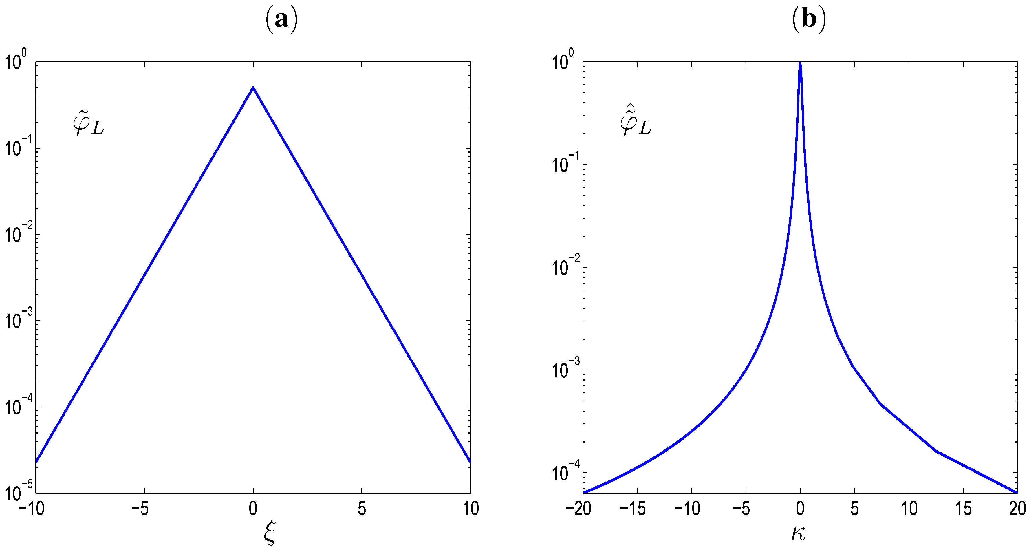
3.1. Fourier Transforms

Let us consider a finite element spatial discretization of the geometrical domain where the representative mesh size is equal to h. In the case of regularized functions with compact support ${\ell }_{\rho }$ we can write ${\ell }_{\rho }=mh$ where m is a positive integer or non-integer number. Tornberg and Engquist [19] proved that, whenever m is a non-integer number in the one-dimensional case, or, alternatively, the two-dimensional and the three-dimensional cases are considered, the error Equation (11) does not decrease for decreasing mesh size. This drawback was discussed by taking into consideration the discrete form of the first moment condition—also denoted as mass condition—whose satisfaction is necessary in order for the regularized formulation to preserve homogeneous fields. Zahedi and Tornberg [22] showed that, even in the one-dimensional case, simple compact support functions such as the hat function or the cosine function lead to a satisfying convergence in the one-dimensional case when $m=1$ and half the support is taken equal to $mh$. However, compact support functions fail to satisfy the mass condition for any non-integer m. In the two-dimensional and the three-dimensional case, this limitation becomes more evident [19]. This is because the number of quadrature points within the support is not constant, but it changes depending on the discretization and the geometry of the interface with respect to the mesh. It should be emphasized that, though effective, we are not focusing on mesh adaptive schemes [3]. We consider instead meshes that do not necessarily conform to the interface position, in line with the spirit of the XFEM [24]. If we choose indeed compact support functions, the width of the support will depend on the position of the interface with respect to the mesh. Consequently, the mesh has to conform to the weight function.

In order to discuss the accuracy of the quadrature procedure, we exploit the results recently obtained by [22] based on the Fourier transforms $\widehat{\phi }$ of φ

$$\widehat{\phi }\left(\kappa \right)={\int }_{-\infty }^{\infty }\phi \left(\xi \right)e^{-2\pi i\kappa \xi }d\xi$$

(13)

Conversely, we have that

$$\phi \left(\xi \right)={\int }_{-\infty }^{\infty }\widehat{\phi }\left(\kappa \right)e^{2\pi i\kappa \xi }d\kappa$$

(14)

Under the hypothesis that the space is covered by a regular grid $\left\{{\mathbf{x}}_j\right\}$, with $j\in \mathbb{Z}$, of quadrature points, Zahedi and Tornberg [22] showed that the discrete version of the moment conditions (12) is related to the derivatives of the Fourier transform $\widehat{\phi }$ as follows

$$M_r({\delta }_{\rho },h)=\frac{1}{{(-2\pi i)}^r}\frac{{\partial }^r\widehat{\phi }\left(m\kappa \right)}{\partial {\kappa }^r}{|}_{\kappa =0}+\frac{1}{{(-2\pi i)}^r}\sum _{\kappa \in \mathbb{Z},\kappa \ne 0}{e}^{-2\pi i\kappa p}\frac{{\partial }^r\widehat{\phi }\left(m\kappa \right)}{\partial {\kappa }^r}$$

(15)

Now, suppose that $\widehat{\phi }\left(\kappa \right)\approx 0$ for $\kappa \ge \beta$; consequently, the last term on the r.h.s. of Equation (15)

$$e^{-2\pi i\kappa p}\frac{{\partial }^r\widehat{\phi }\left(m\right)}{\partial {\kappa }^r}+e^{-2\pi i\kappa p}\frac{{\partial }^r\widehat{\phi }\left(2m\right)}{\partial {\kappa }^r}+\dots$$

(16)

turns out to vanish for any $m\ge \lambda$. Hence if the conditions

$$\frac{{\partial }^r}{\partial {\kappa }^r}\widehat{\phi }\left(\kappa \right){{|}_{\kappa =0}=1,\text{for}r=0,\frac{{\partial }^r}{\partial {\kappa }^r}\widehat{\phi }\left(\kappa \right)|}_{\kappa =0}=0\text{for}1\le r<q$$

(17)

are satisfied for $r=0,1,\dots ,q-1$, then ${\delta }_{\rho }$ satisfies q discrete moment conditions. In particular, if $\widehat{\phi }\left(0\right)=1$, the mass condition

$${\int }_{-\infty }^{\infty }{\phi }_{\rho }\left(x\right)dx=\widehat{\phi }\left(0\right)=1$$

(18)

is satisfied [19]. Moreover, the derivatives of the Fourier transform and the moment conditions on φ are related by the relationship $\frac{{\partial }^r\widehat{\phi }}{\partial {\kappa }^r}{|}_{\kappa =0}={(-i)}^p{\int }_{-\infty }^{\infty }\phi \left(\xi \right){\xi }^{r}d\xi$. Hence the relationships

$$\frac{{\partial }^r\widehat{\phi }\left(\kappa \right)}{\partial {\kappa }^r}{|}_{\kappa =0}=0\iff {\int }_{-\infty }^{\infty }\phi \left(\xi \right){\xi }^{r}d\xi =0$$

(19)

hold for any $r>1$. Note that the Fourier transform of a compact support weight function is generally non-compact [22].

3.2. Truncation Error

Considering that the support of a non-compact support function will be truncated at a certain distance from the interface Γ, truncation will introduce a further source of approximation. However, it can be shown that the analytical error decreases for decreasing mesh size h while this does not generally happen in the case of compact support functions. However, the analytical error mainly depends on the truncation error, which is introduced in neglecting the contributions of quadrature points placed beyond a certain distance [22]. Hence we can fix ρ independently of the mesh size and increase the support until the numerical error is below an acceptable value.

To recapitulate, we have two possibilities:

• we choose weight functions with compact support equal to the finite element size multiplied by a suitable integer number m that depends on h, namely ${\ell }_{\rho }\propto mh$ [1,3]. This means that whenever the mesh changes, the weight function has to be changed accordingly, otherwise non-vanishing errors for decreasing mesh size are obtained.
• we choose non-compact support weight functions whose Fourier transform $\widehat{\phi }$ satisfies differentiability conditions; the length ${\ell }_{\rho }$ will denote the truncated support of φ. This makes it possible to have ${\ell }_{\rho }$ independent of h when ${\ell }_{\rho }\ge {\gamma }_{\widehat{\phi }}h$, where ${\gamma }_{\widehat{\phi }}$ is the width of the truncated support of the Fourier transform $\widehat{\phi }$.

We want to investigate option 2. This requires evaluating the error due to truncation of the weight function. Denote the truncated delta function ${\delta }_{\rho }^{\omega }$ as

$${\delta }_{\rho }^{\omega }\left(t\right)=\left\{\begin{array}{cc}{\delta }_{\rho }\left(t\right)\hfill & \text{for}t\in [-\omega ,\omega ]\hfill \\ 0\hfill & \text{otherwise}\hfill \end{array}\right.$$

(20)

where $w={\ell }_{\rho }/2$, ${\ell }_{\rho }$ being the width of the truncated support of the weight function. Tornberg and Engquist [19] showed that the analytical error ${\mathcal{ℰ}}_{\omega }$ associated with truncation can be neglected provided that

$$\begin{array}{cc}& {\int }_{-\omega }^{\omega }{\delta }_{\rho }^{\omega }\left(t\right)dt=1\hfill \end{array}$$

(21a)

$$\begin{array}{cc}& {\int }_{-\omega }^{\omega }{\delta }_{\rho }^{\omega }\left(t\right)tdt=0\hfill \end{array}$$

(21b)

As ${\delta }_{\rho }^{\omega }$ is even then

$${\int }_{-\infty }^{-\omega }{\delta }_{\rho }\left(t\right)tdt+{\int }_{\omega }^{\infty }{\delta }_{\rho }\left(t\right)tdt=0$$

(22)

Consequently,

$${\int }_{-\infty }^{\infty }{\delta }_{\rho }\left(t\right)tdt={\int }_{-\infty }^{-\omega }{\delta }_{\rho }\left(t\right)tdt+{\int }_{\omega }^{\infty }{\delta }_{\rho }\left(t\right)tdt+{\int }_{-\omega }^{\omega }{\delta }_{\rho }^{\omega }\left(t\right)tdt=0$$

(23)

Therefore Equation (23) implies that the truncated weight function satisfies the moment condition (21b). In order to prove condition (21a), we estimate

$$I_1+I_2={\int }_{-\infty }^{-\omega }{\delta }_{\rho }\left(t\right)dt+{\int }_{\omega }^{\infty }{\delta }_{\rho }\left(t\right)dt$$

(24)

For instance taking $\phi =e^{-\frac{\left|t\right|}{\rho }}$ leads to $I_1=I_2=\rho e^{-\frac{\omega }{\rho }}$. Hence the analytical error decreases for increasing support width ${\ell }_{\rho }=2\omega$. The maximum value of the error, equal to ρ, is reached for $\omega =0$. In the following we will omit ω and use ${\delta }_{\rho }$ to indicate the truncated regularized delta.

3.3. Example

In Table 2, we compare the Fourier transforms and the corresponding derivatives of modified versions ${\tilde{\phi }}_L$ and ${\tilde{\phi }}_G$ of the exponential and the Gauß weight functions, respectively. The Fourier transform was calculated using the forward definition (13) [26]. The weight function ${\tilde{\phi }}_L\left(t\right)=(1/2)e^{-\left|\xi \right|}$ where $\xi =\frac{t}{\rho }$ and its Fourier transform ${\widehat{\tilde{\phi }}}_L\left(\kappa \right)$ are compared in Figure 1. We can note that ${\widehat{\tilde{\phi }}}_L\left(\kappa \right)\le {10}^{-4}$ for $\kappa \ge 20$, which suggests that we can reach at maximum the accuracy ${10}^{-4}$ if we truncate the weight function ${\phi }_L$ assuming $\rho \ge 20h$. The value $20h$ provides an upper bound for ρ, any smaller value of ρ should be discarded.

Table 2. Fourier transforms of two weight functions.

$\phi \left(\xi \right)$	$\widehat{\phi }\left(\kappa \right)$	$\widehat{\phi }\left(0\right)$	${\displaystyle \frac{\partial \widehat{\phi }}{\partial \kappa }{|}_{\kappa =0}}$	${\displaystyle \frac{{\partial }^2\widehat{\phi }}{\partial {\kappa }^2}{|}_{\kappa =0}}$
${\tilde{\phi }}_L=\frac{1}{2}{e}^{-\left|\xi \right|}$	${\displaystyle \frac{1}{1+4{\pi }^2{\kappa }^2}}$	1	0	$\ne 0$
${\tilde{\phi }}_G=2\sqrt{\pi }{e}^{-4{\pi }^2{\xi }^2}$	${\displaystyle e^{\frac{-{\kappa }^2}{4}}}$	1	0	$\ne 0$

Table 2. Fourier transforms of two weight functions.

$\phi \left(\xi \right)$	$\widehat{\phi }\left(\kappa \right)$	$\widehat{\phi }\left(0\right)$	${\displaystyle \frac{\partial \widehat{\phi }}{\partial \kappa }{|}_{\kappa =0}}$	${\displaystyle \frac{{\partial }^2\widehat{\phi }}{\partial {\kappa }^2}{|}_{\kappa =0}}$
${\tilde{\phi }}_L=\frac{1}{2}{e}^{-\left|\xi \right|}$	${\displaystyle \frac{1}{1+4{\pi }^2{\kappa }^2}}$	1	0	$\ne 0$
${\tilde{\phi }}_G=2\sqrt{\pi }{e}^{-4{\pi }^2{\xi }^2}$	${\displaystyle e^{\frac{-{\kappa }^2}{4}}}$	1	0	$\ne 0$

Figure 1. (a) Exponential weight function ${\tilde{\phi }}_L=1/2e^{-\left|\xi \right|}$; (b) Fourier transform ${\widehat{\tilde{\phi }}}_L={\displaystyle \frac{1}{1+4{\pi }^2{\kappa }^2}}$. The vertical axis is in log-scale.

Figure 1. (a) Exponential weight function ${\tilde{\phi }}_L=1/2e^{-\left|\xi \right|}$; (b) Fourier transform ${\widehat{\tilde{\phi }}}_L={\displaystyle \frac{1}{1+4{\pi }^2{\kappa }^2}}$. The vertical axis is in log-scale.

According to the previous results, ${\tilde{\phi }}_L$ and ${\tilde{\phi }}_G$ satisfy the moment conditions up to order 2. We have checked that the results pertaining to the width of the support of the simplified weight functions ${\tilde{\phi }}_L$ and $\widetilde{{\phi }_G}$ can be extended to the weight functions ${\phi }_L$ and ${\phi }_G$. In the numerical analysis, ${\phi }_L=e^{-\left|\xi \right|}$ is exploited, the discussion of the case ${\phi }_G$ is part of a research in progress.

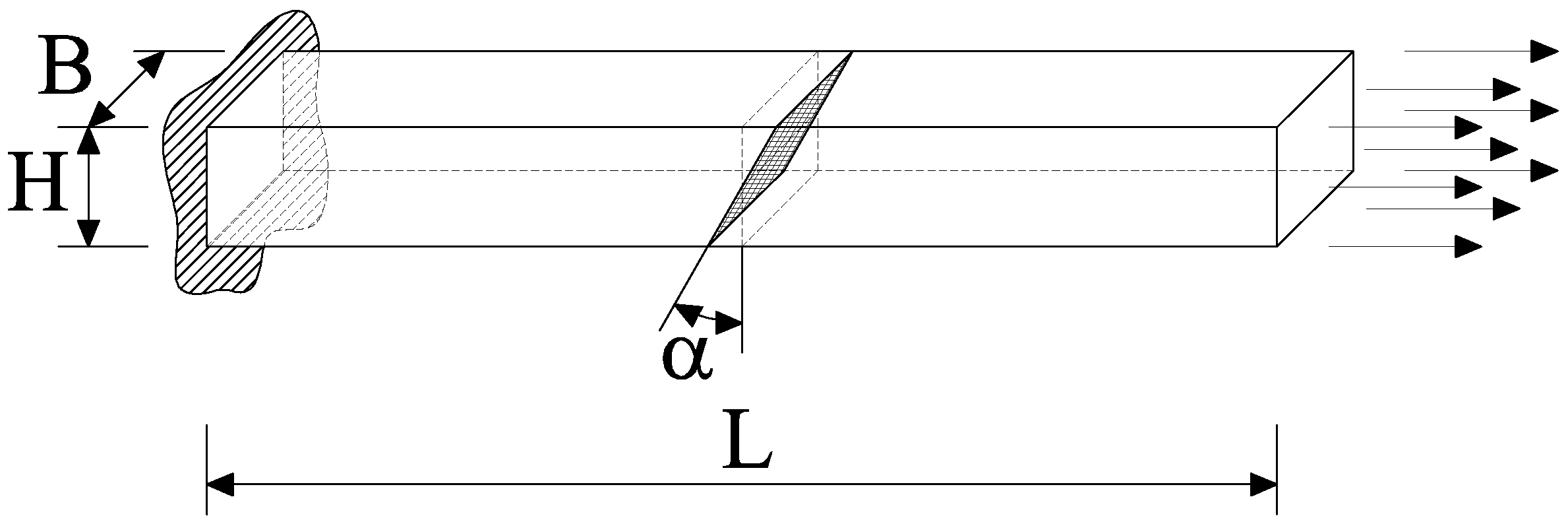
4. Basic Statements of the Regularized XFEM Formulation

We consider a regularized XFEM developed for strain localization and cohesive interfaces [13,17,27]. The displacement field is approximated by enriching the space of the shape functions with additional functions that fulfill the partition of unity property of the standard finite element method. The enrichment functions consist of the product of the Heaviside function by the standard shape functions N

$$\mathbf{u}\left(\mathbf{x}\right)=\mathbf{N}\left(\mathbf{x}\right)\mathbf{V}+\mathscr{H}\left(d\right(\mathbf{x}\left)\right)\mathbf{N}\left(\mathbf{x}\right)\mathbf{J}$$

(25)

In Equation (25), V is the vector containing the degrees of freedom of the standard part of the displacement field v, while J collects the enriched degrees of freedom related to the displacement jump across the interface. The strain field is computed via compatibility from Equation (25) as

$$\epsilon \left(\mathbf{x}\right)=\mathbf{B}\left(\mathbf{x}\right)\mathbf{V}+\mathscr{H}\left(d\left(\mathbf{x}\right)\right)\mathbf{B}\left(\mathbf{x}\right)\mathbf{J}+\delta \left(d\left(\mathbf{x}\right)\right)\overline{\mathbf{N}}\left(\mathbf{x}\right)\mathbf{J}$$

(26)

where B is the compatibility matrix, $\overline{\mathbf{N}}$ is related to the term in Equation (3) containing the (generalized) gradient $\nabla \mathscr{H}=\delta \mathbf{n}$. Following the methodology proposed in [13,17] regularization is carried out. The regularized displacement and strain fields become

$$\begin{array}{cc}\hfill {\mathbf{u}}_{\rho }\left(\mathbf{x}\right)& =\mathbf{N}\left(\mathbf{x}\right)\mathbf{V}+{\mathscr{H}}_{\rho }\left(d\left(\mathbf{x}\right)\right)\mathbf{N}\left(\mathbf{x}\right)\mathbf{J}\hfill \end{array}$$

(27a)

$$\begin{array}{cc}\hfill {\epsilon }_{\rho }\left(\mathbf{x}\right)& ={\epsilon }_a\left(\mathbf{x}\right)+{\epsilon }_b\left(\mathbf{x}\right)\hfill \end{array}$$

(27b)

where

$$\begin{array}{cc}\hfill {\epsilon }_a\left(\mathbf{x}\right)& =\mathbf{B}\left(\mathbf{x}\right)\mathbf{V}+{\mathscr{H}}_{\rho }\left(d\left(\mathbf{x}\right)\right)\mathbf{B}\left(\mathbf{x}\right)\mathbf{J}\hfill \end{array}$$

(28a)

$$\begin{array}{cc}\hfill {\epsilon }_b\left(\mathbf{x}\right)& ={\delta }_{\rho }\left(d\left(\mathbf{x}\right)\right)\overline{\mathbf{N}}\left(\mathbf{x}\right)\mathbf{J}\hfill \end{array}$$

(28b)

Let the material occupying volume V be elastic with Young’s modulus E. The regularized interface is characterized by the Young’s modulus by unit length $\overline{\mathbf{E}}/{\delta }_{\rho }=\mathbf{E}/\left(\beta {\delta }_{\rho }\right)$, where $\beta <1$ and $\beta >1$ mean that the regularized interface is weaker or stronger, respectively, than the bulk, while for $\beta =1$ the Young’s moduli of the interface and the bulk coincide. The dimensional consistency and the motivations for assuming $\overline{\mathbf{E}}$ in this way were thoroughly discussed in [17]. Let us omit the spatial dependence. It was proved in [17] that the internal virtual work has to be assumed as

$$\begin{array}{cc}& {\int }_V{\sigma }_a·{\epsilon }_a+{\sigma }_b·{\epsilon }_{b}dV=\hfill \\ & {\int }_V(\mathbf{E}\mathbf{B}\mathbf{V}+{\mathscr{H}}_{\rho }\mathbf{E}\mathbf{B}\mathbf{J})·(\mathbf{B}\mathbf{V}+{\mathscr{H}}_{\rho }\mathbf{B}\mathbf{J})dV+{\int }_V\left(\overline{\mathbf{E}}\overline{\mathbf{N}}\mathbf{J}\right)·\left({\delta }_{\rho }\overline{\mathbf{N}}\mathbf{J}\right)dV=\hfill \\ & {\int }_V{\mathbf{B}}^t\mathbf{E}\mathbf{B}dV\mathbf{V}·\mathbf{V}+{\int }_V{\mathscr{H}}_{\rho }{\mathbf{B}}^t\mathbf{E}\mathbf{B}dV\mathbf{J}·\mathbf{V}+{\int }_V{\mathscr{H}}_{\rho }{\mathbf{B}}^t\mathbf{E}\mathbf{B}dV\mathbf{V}·\mathbf{J}+\hfill \\ & {\int }_V{\mathscr{H}}_{\rho }^2{\mathbf{B}}^t\mathbf{E}\mathbf{B}dV\mathbf{J}·\mathbf{J}+{\int }_{V_{\rho }}{\delta }_{\rho }{\overline{\mathbf{N}}}^t\overline{\mathbf{E}}\overline{\mathbf{N}}dV\mathbf{J}·\mathbf{J}\hfill \end{array}$$

(29)

where the constitutive laws

$$\begin{array}{cc}& {\sigma }_a=\mathbf{E}{\epsilon }_a=\mathbf{E}\mathbf{B}\mathbf{V}+\mathbf{E}{\mathscr{H}}_{\rho }\mathbf{B}\mathbf{J},\hfill \end{array}$$

(30a)

$$\begin{array}{cc}& {\sigma }_b=\overline{\mathbf{E}}{\epsilon }_b=\overline{\mathbf{E}}\mathbf{N}\mathbf{J}\hfill \end{array}$$

(30b)

are adopted. Equation (29) can be written in a more compact form as

$${\int }_V\sigma ·\epsilon dV={\int }_V\mathbf{u}·\mathbf{K}\mathbf{u}dV$$

(31)

where the stiffness matrix

$$\mathbf{K}=\left(\begin{array}{cc}{\mathbf{K}}_{vv}& {\mathbf{K}}_{vj}\\ {\mathbf{K}}_{jv}& {\mathbf{K}}_{jj}\end{array}\right)$$

(32)

collects the following submatrices

$$\begin{array}{cccccc}\hfill {\mathbf{K}}_{vv}={\mathbf{B}}^t\mathbf{E}\mathbf{B},& & \hfill {\mathbf{K}}_{jv}& ={\mathscr{H}}_{\rho }{\mathbf{B}}^t\mathbf{E}\mathbf{B}={\mathbf{K}}_{ja}^t,\hfill & & {\mathbf{K}}_{jj}={\delta }_{\rho }{\overline{\mathbf{N}}}^t\overline{\mathbf{E}}\overline{\mathbf{N}}+{\mathscr{H}}_{\rho }^2{\mathbf{B}}^t\mathbf{E}\mathbf{B}\hfill \end{array}$$

(33)

The model has been implemented in X3D^©, a Fortran three-dimensional code based on the eXtended Finite Element method. All the submatrices (33) were computed by means of standard Gauß quadrature. More details on the quadrature procedure are given in Section 5.

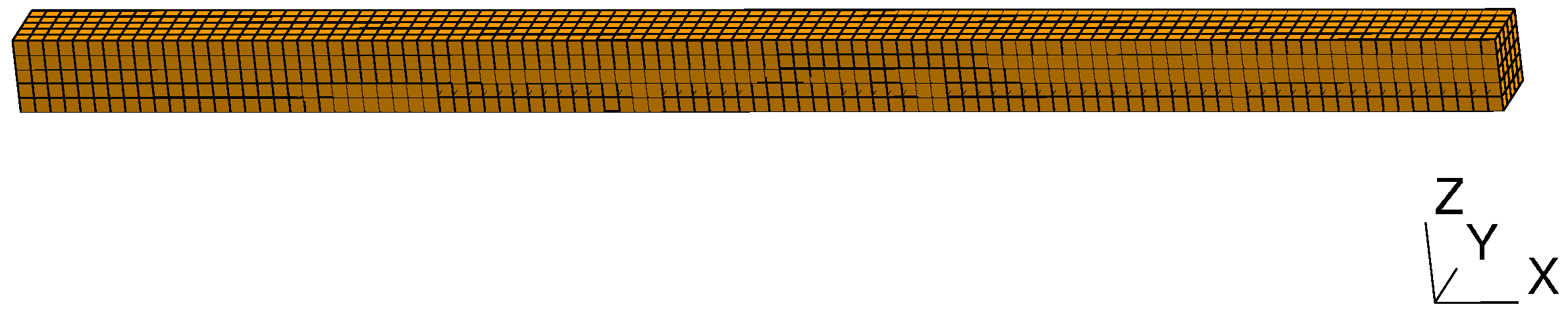
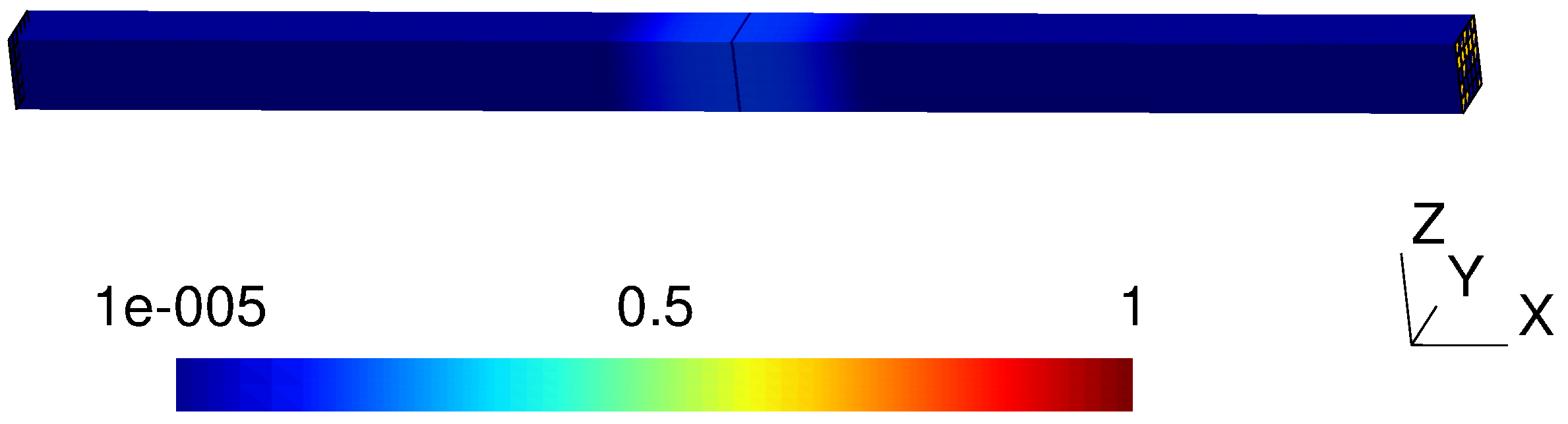
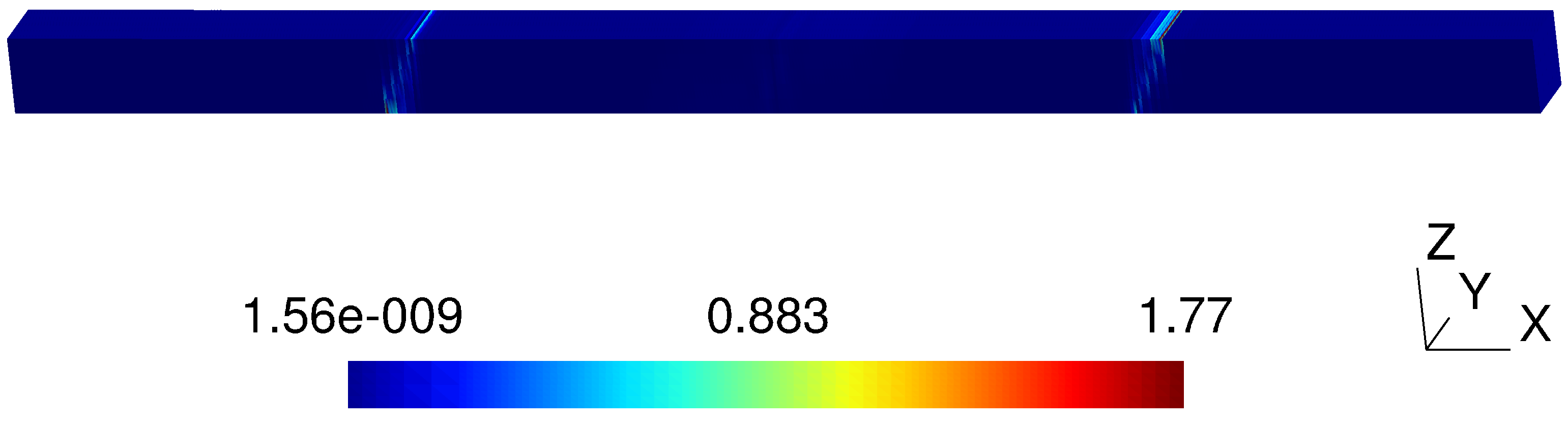
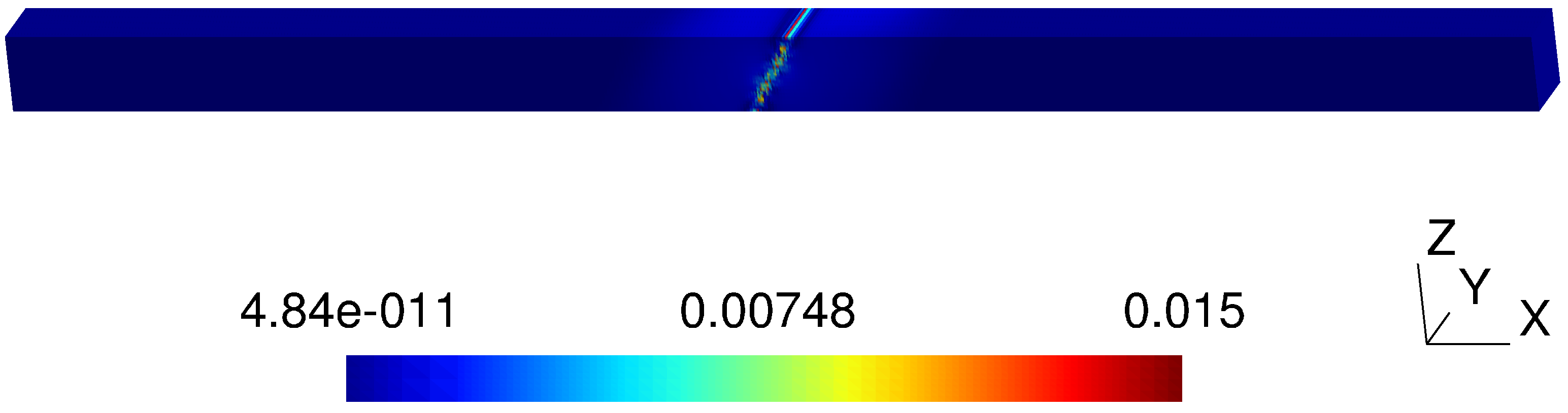
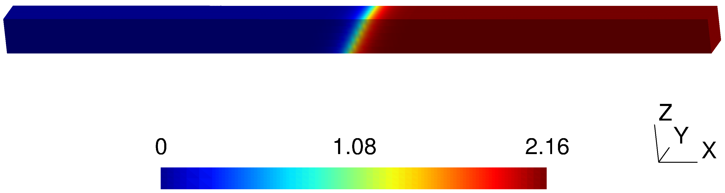
5. Numerical Results

The accuracy of the proposed model is evaluated by considering the slender three-dimensional solid shown in Figure 2 with length $L=2$ cm, cross section $A=H\times B$, $H=B=L/10$. The element is clamped at one end and subjected to load control at the free end. An interface at $L/2$ is placed. Meshes of hexahedra are considered consisting of at least $5\times 5$ elements in the cross section and increasing number of elements along the loading direction (see Figure 3). Enriched hexahedra possess a quadrature grid of $8^3$ Gauß points, while non-enriched hexahedra contain $2^3$ Gauß points. The analytical solution predicts a uniform state of stress along the loading direction. The uniform norm of the error, namely the maximal error on the stress component ${\sigma }_{xx}$

$$\mathcal{ℰ}=\frac{\parallel {\sigma }_{xx}-{\sigma }_{xx}^h{\parallel }_{\infty }}{{\sigma }_{xx}}$$

(34)

is evaluated [23]. The parameter β characterizing the ratio between the Young’s modulus of the bulk and that of the interface is set equal to ${10}^{-4}$.

Figure 2. Geometry of the uniaxial test.

Figure 2. Geometry of the uniaxial test.

Figure 3. Typical mesh.

Figure 3. Typical mesh.

Table 3 and Table 4 illustrate the errors obtained in the case of vertical interface with $\alpha =0^{\circ }$ for fixed ρ and fixed h, respectively. In both cases, the support width ${\ell }_{\rho }=20\rho$ was adopted. The ratio $\rho /h$ is incremented, in the former case by decreasing h, and in the latter case by increasing ρ. Figure 4 displays the error in percentage for the case of $\rho =L/100$, $\rho /h=5$ and the support width ${\ell }_{\rho }=20\rho$.

Table 3. Error for decreasing h, fixed $\rho =L/100$, vertical discontinuity $\alpha =0^{\circ }$; the support width is ${\ell }_{\rho }=20\rho$.

Mesh	$\rho /h$	$ℰ$
$5\times 5\times 5$	$5.2\times {10}^{-2}$	0.42
$9\times 5\times 5$	$9.4\times {10}^{-2}$	0.18
$19\times 5\times 5$	$2\times {10}^{-1}$	$6\times {10}^{-2}$
$55\times 5\times 5$	$5.7\times {10}^{-1}$	$2\times {10}^{-2}$
$99\times 5\times 5$	1.0	$1\times {10}^{-2}$
$255\times 5\times 5$	2.6	$3\times {10}^{-3}$
$500\times 5\times 5$	5.2	$2\times {10}^{-3}$
$749\times 5\times 5$	7.8	$1\times {10}^{-3}$
$999\times 5\times 5$	10.5	$9\times {10}^{-4}$
$1499\times 5\times 5$	16.5	$6\times {10}^{-4}$

Table 3. Error for decreasing h, fixed $\rho =L/100$, vertical discontinuity $\alpha =0^{\circ }$; the support width is ${\ell }_{\rho }=20\rho$.

Mesh	$\rho /h$	$ℰ$
$5\times 5\times 5$	$5.2\times {10}^{-2}$	0.42
$9\times 5\times 5$	$9.4\times {10}^{-2}$	0.18
$19\times 5\times 5$	$2\times {10}^{-1}$	$6\times {10}^{-2}$
$55\times 5\times 5$	$5.7\times {10}^{-1}$	$2\times {10}^{-2}$
$99\times 5\times 5$	1.0	$1\times {10}^{-2}$
$255\times 5\times 5$	2.6	$3\times {10}^{-3}$
$500\times 5\times 5$	5.2	$2\times {10}^{-3}$
$749\times 5\times 5$	7.8	$1\times {10}^{-3}$
$999\times 5\times 5$	10.5	$9\times {10}^{-4}$
$1499\times 5\times 5$	16.5	$6\times {10}^{-4}$

Table 4. Error for increasing ρ, fixed $h=L/749$ corresponding to the $749\times 5\times 5$ mesh, inclination of the vertical discontinuity $\alpha =0^{\circ }$; the support width is ${\ell }_{\rho }=20\rho$.

$\rho /h$	$ℰ$
$4.9\times {10}^{-2}$	$4.0\times {10}^{-1}$
$1.5\times {10}^{-1}$	$8.7\times {10}^{-2}$
$3.5\times {10}^{-1}$	$2.8\times {10}^{-2}$
$5.4\times {10}^{-1}$	$1.7\times {10}^{-2}$
$7.4\times {10}^{-1}$	$1.2\times {10}^{-2}$
1	$8.4\times {10}^{-3}$
2.5	$3.5\times {10}^{-3}$
4.8	$1.8\times {10}^{-3}$
7.8	$1.2\times {10}^{-3}$
17.3	$5.5\times {10}^{-4}$
37	$2.9\times {10}^{-4}$

Table 4. Error for increasing ρ, fixed $h=L/749$ corresponding to the $749\times 5\times 5$ mesh, inclination of the vertical discontinuity $\alpha =0^{\circ }$; the support width is ${\ell }_{\rho }=20\rho$.

$\rho /h$	$ℰ$
$4.9\times {10}^{-2}$	$4.0\times {10}^{-1}$
$1.5\times {10}^{-1}$	$8.7\times {10}^{-2}$
$3.5\times {10}^{-1}$	$2.8\times {10}^{-2}$
$5.4\times {10}^{-1}$	$1.7\times {10}^{-2}$
$7.4\times {10}^{-1}$	$1.2\times {10}^{-2}$
1	$8.4\times {10}^{-3}$
2.5	$3.5\times {10}^{-3}$
4.8	$1.8\times {10}^{-3}$
7.8	$1.2\times {10}^{-3}$
17.3	$5.5\times {10}^{-4}$
37	$2.9\times {10}^{-4}$

Figure 4. Error $ℰ$(34) in % for the $\alpha =0^{\circ }$ discontinuity, $h=L/500$, $\rho /h=5$ and support width ${\ell }_{\rho }=20\rho$.

Figure 4. Error $ℰ$(34) in % for the $\alpha =0^{\circ }$ discontinuity, $h=L/500$, $\rho /h=5$ and support width ${\ell }_{\rho }=20\rho$.

The same analysis is repeated for one case of inclined interface, namely $\alpha ={30}^{\circ }$. The corresponding results are reported in Table 5 and Table 6. In Table 5, the mesh of 255 elements along the length was refined in the cross section in order to reduce mesh distortion [28]. In particular, in Table 6, the influence on the numerical error of the support width is illustrated. While here, unlike in the case $\alpha =0^{\circ }$, the support width ${\ell }_{\rho }=20\rho$ leads to non-satisfying results, the minimal error obtained by adopting a support ${\ell }_{\rho }=40\rho$ is of the order ${10}^{-3}$, while the quality of the convergence is non-satisfying as $ℰ$ oscillates. Conversely, adoption of ${\ell }_{\rho }=60\rho$ improves convergence. Note that in Table 5 and Table 6, a smaller value of the ratio $\rho /h$ is used than in Table 5, because larger ρ may lead to ${\ell }_{\rho }$ larger than the length L. The map of the stress error in percentage for varying truncated support width are displayed in Figure 5 and Figure 6, corresponding to ${\ell }_{\rho }=40\rho$ and ${\ell }_{\rho }=60\rho$, respectively. In the former figure, the total error is dominated by the truncation error, because it is localized at the enriched volume boundary. In the latter figure, the truncation error disappears, while the relevant error is localized along the inclined interface. In both figures, the ratio $\rho /h=5$ is used. Consequently, the enrichment involves several layers of elements. This reflects the fact that the displacement jump across the discontinuity is smeared over a width larger than the representative element size, as shown in Figure 7.

Table 5. Error for decreasing h, fixed $\rho =L/100$, $\alpha ={30}^{\circ }$, support width ${\ell }_{\rho }=40\rho$.

Mesh	$\rho /h$	$ℰ$
$5\times 5\times 5$	$5.2\times {10}^{-2}$	$3.1\times {10}^{-1}$
$9\times 5\times 5$	$9.4\times {10}^{-2}$	$3.8\times {10}^{-2}$
$19\times 5\times 5$	$2\times {10}^{-1}$	$3\times {10}^{-3}$
$55\times 5\times 5$	$5.7\times {10}^{-1}$	$3.2\times {10}^{-4}$
$99\times 5\times 5$	1.0	$5.5\times {10}^{-4}$
$255\times 5\times 20$	2.6	$1.6\times {10}^{-4}$

Table 5. Error for decreasing h, fixed $\rho =L/100$, $\alpha ={30}^{\circ }$, support width ${\ell }_{\rho }=40\rho$.

Mesh	$\rho /h$	$ℰ$
$5\times 5\times 5$	$5.2\times {10}^{-2}$	$3.1\times {10}^{-1}$
$9\times 5\times 5$	$9.4\times {10}^{-2}$	$3.8\times {10}^{-2}$
$19\times 5\times 5$	$2\times {10}^{-1}$	$3\times {10}^{-3}$
$55\times 5\times 5$	$5.7\times {10}^{-1}$	$3.2\times {10}^{-4}$
$99\times 5\times 5$	1.0	$5.5\times {10}^{-4}$
$255\times 5\times 20$	2.6	$1.6\times {10}^{-4}$

Table 6. Error for increasing ρ, various support widths ${\ell }_{\rho }$, fixed $h=L/749$ in a $749\times 5\times 5$ mesh, and inclined interface with $\alpha ={30}^{\circ }$.

$\rho /h$	${\mathcal{E}}_{{\ell }_{\rho }=20\rho }$	${\mathcal{E}}_{{\ell }_{\rho }=40\rho }$	${\mathcal{ℰ}}_{{\ell }_{\rho }=60\rho }$
$4.9\times {10}^{-2}$	$>10$	$1.4\times {10}^{-1}$	$1.4\times {10}^{-1}$
$1.5\times {10}^{-1}$	$>10$	$2.2\times {10}^{-2}$	$2.2\times {10}^{-2}$
$3.5\times {10}^{-1}$	$>10$	$6.7\times {10}^{-3}$	$6.8\times {10}^{-3}$
$5.4\times {10}^{-1}$	$>10$	$4.2\times {10}^{-3}$	$4.4\times {10}^{-3}$
$7.4\times {10}^{-1}$	$>10$	$9.6\times {10}^{-3}$	$3.1\times {10}^{-3}$
1	$>10$	$1\times {10}^{-2}$	$1.9\times {10}^{-3}$
2.5	$>10$	$8.4\times {10}^{-3}$	$2.8\times {10}^{-4}$
4.8	$>10$	$7.7\times {10}^{-3}$	$2.7\times {10}^{-4}$
7.8	$>10$	$6.4\times {10}^{-3}$	$2.1\times {10}^{-4}$

Table 6. Error for increasing ρ, various support widths ${\ell }_{\rho }$, fixed $h=L/749$ in a $749\times 5\times 5$ mesh, and inclined interface with $\alpha ={30}^{\circ }$.

$\rho /h$	${\mathcal{E}}_{{\ell }_{\rho }=20\rho }$	${\mathcal{E}}_{{\ell }_{\rho }=40\rho }$	${\mathcal{ℰ}}_{{\ell }_{\rho }=60\rho }$
$4.9\times {10}^{-2}$	$>10$	$1.4\times {10}^{-1}$	$1.4\times {10}^{-1}$
$1.5\times {10}^{-1}$	$>10$	$2.2\times {10}^{-2}$	$2.2\times {10}^{-2}$
$3.5\times {10}^{-1}$	$>10$	$6.7\times {10}^{-3}$	$6.8\times {10}^{-3}$
$5.4\times {10}^{-1}$	$>10$	$4.2\times {10}^{-3}$	$4.4\times {10}^{-3}$
$7.4\times {10}^{-1}$	$>10$	$9.6\times {10}^{-3}$	$3.1\times {10}^{-3}$
1	$>10$	$1\times {10}^{-2}$	$1.9\times {10}^{-3}$
2.5	$>10$	$8.4\times {10}^{-3}$	$2.8\times {10}^{-4}$
4.8	$>10$	$7.7\times {10}^{-3}$	$2.7\times {10}^{-4}$
7.8	$>10$	$6.4\times {10}^{-3}$	$2.1\times {10}^{-4}$

Figure 5. Error $ℰ$(34) in % for the $\alpha ={30}^{\circ }$ discontinuity, $h=L/500$, $\rho /h=5$ and support width ${\ell }_{\rho }=40\rho$. Note that the truncation error is dominant.

Figure 5. Error $ℰ$(34) in % for the $\alpha ={30}^{\circ }$ discontinuity, $h=L/500$, $\rho /h=5$ and support width ${\ell }_{\rho }=40\rho$. Note that the truncation error is dominant.

Figure 6. Error $ℰ$(34) in % for the $\alpha ={30}^{\circ }$ discontinuity, $h=L/500$, $\rho /h=5$ and support width ${\ell }_{\rho }=60\rho$. Note that the relevant error is localized along the inclined interface.

Figure 6. Error $ℰ$(34) in % for the $\alpha ={30}^{\circ }$ discontinuity, $h=L/500$, $\rho /h=5$ and support width ${\ell }_{\rho }=60\rho$. Note that the relevant error is localized along the inclined interface.

Figure 7. Displacement μ_x for the $\alpha ={30}^{\circ }$ discontinuity, $h=L/500$, $\rho /h=5$ and support width ${\ell }_{\rho }=40\rho$.

Figure 7. Displacement μ_x for the $\alpha ={30}^{\circ }$ discontinuity, $h=L/500$, $\rho /h=5$ and support width ${\ell }_{\rho }=40\rho$.

We have obtained a level-set dependent delta function approximation ${\delta }_{\rho }$. The function ${\delta }_{\rho }$ satisfies three moment conditions up to a precision C when $\widehat{\phi }\left(\kappa \right)\le C$ for any $\kappa \ge C$. This circumstance occurs if the ratio $\rho /h$ is greater than 20. Moreover, the width of the support width ${\ell }_{\rho }$ should be chosen at least equal to $40\rho$ in order to contain the truncation error. Hence, we can conclude that, generally, the support width should be larger than $40\rho$.

5.1. Algorithm

An algorithmic scheme taking into account the previous analysis is the following:

Step 1 Fix the tolerance parameters C, $C_{\mathcal{E}}$

Step 2 Evaluate β such that $\widehat{\phi }\left(\beta \right)\le C$

Step 3 Assume $\rho =\beta h$, ${\ell }_{\rho }=m\rho$, $i=0$

Step 4 Perform the analysis and evaluate $ℰ$.

while $\mathcal{E}>C_{\mathcal{E}}$

set ${\ell }_{\rho }=im\rho$;

$i=i+1$.

end while

6. Conclusions

In this paper, Gauß quadrature was used in a three-dimensional XFEM analysis of regularized interfaces. The relationship between Fourier transforms of the weight function and the analytical error was exploited. The main advantages are the simplicity of the approach and the fact that adaptive remeshing and quadrature are avoided. The numerical accuracy of regularized non-compact support was discussed in a benchmark test consisting of a 3D slender solid subjected to a tensile loading. The truncated support width ${\ell }_{\rho }$ and the ratio $\rho /h$ are the main parameters to be considered for controlling the approximation. It was shown that non-compact support weight functions make it possible to get a reasonable accuracy of the results. In particular:

• truncation of the support width ${\ell }_{\rho }$ influences the analytical error, as the moment conditions (12) are not exactly satisfied;
• the computed error $ℰ$ decreases for increasing values of the ratio $\rho /h$, that is either increasing ρ for fixed h or decreasing h for fixed ρ;
• discontinuities and singularities along interfaces that are non-aligned with the mesh are prone to severe errors when the support width ${\ell }_{\rho }<40\rho$.

The results shown in this contribution are part of an ongoing research on general quadrature procedures for discontinuous and singular functions in three-dimensional structural problems.

References

1. Abbas, S.; Alizada, A.; Fries, T. The XFEM for high-gradient solutions in convection-dominated problems. Int. J. Numer. Methods Eng. 2010, 82, 1044–1072. [Google Scholar] [CrossRef]
2. Mallardo, V. Integral equations and nonlocal damage theory: A numerical implementation using the BDEM. Int. J. Fract. 2009, 157, 13–32. [Google Scholar] [CrossRef]
3. Mousavi, S.; Pask, J.; Sukumar, N. Efficient adaptive integration of functions with sharp gradients and cusps in n-dimensional parallelepipeds. Int. J. Numer. Methods Eng. 2012, 91, 343–357. [Google Scholar] [CrossRef]
4. Iarve, E.; Gurvich, M.; Mollenhauer, D.; Rose, C.; Dávila, C. Mesh-Independent matrix cracking and delamination modeling in laminated composites. Int. J. Numer. Methods Eng. 2011, 88, 749–773. [Google Scholar] [CrossRef]
5. Xu, J.; Lee, C.; Tan, K. A two-dimensional co-rotational Timoshenko beam element with XFEM formulation. Comput. Mech. 2012, 49, 667–683. [Google Scholar] [CrossRef]
6. Belytschko, T.; Gracie, R.; Ventura, G. A review of the extended/generalized finite element methods for material modelling. Modell. Simul. Mater. Sci. Eng. 2009, 17, 1–24. [Google Scholar]
7. Fries, T.; Belytschko, T. The extended/generalized finite element method: An overview of the method and its applications. Int. J. Numer. Methods Eng. 2010, 84, 253–304. [Google Scholar] [CrossRef]
8. Moës, N.; Dolbow, J.; Belytschko, T. A finite element method for crack growth without remeshing. Int. J. Numer. Methods Eng. 1999, 46, 131–150. [Google Scholar] [CrossRef]
9. Mariani, S.; Perego, U. Extended finite element method for quasi-brittle fracture. Int. J. Numer. Methods Eng. 2003, 58, 103–126. [Google Scholar] [CrossRef]
10. Nikbakht, M.; Wells, G. Automated modelling of evolving discontinuities. Algorithms 2009, 2, 1008–1030. [Google Scholar] [CrossRef]
11. Müller, B.; Kummer, F.; Oberlack, M. Simple multidimensional integration of discontinuous functions with application to level set methods. Int. J. Numer. Methods Eng. 2012, 92, 637–651. [Google Scholar] [CrossRef]
12. Ventura, G. On the elimination of quadrature subcells for discontinuous functions in the eXtended Finite-Element Method. Int. J. Numer. Methods Eng. 2006, 66, 761–795. [Google Scholar] [CrossRef]
13. Benvenuti, E. A regularized XFEM framework for embedded cohesive interfaces. Comput. Methods Appl. Mech. Eng. 2008, 197, 4367–4378. [Google Scholar] [CrossRef]
14. Benvenuti, E.; Tralli, A. Simulation of finite-width process zone for concrete-like materials. Comput. Mech. 2012, 50, 479–497. [Google Scholar] [CrossRef]
15. Benvenuti, E.; Tralli, A. Iterative LCP-solvers for non-local loading-unloading conditions. Int. J. Numer. Methods Eng. 2003, 58, 2343–2370. [Google Scholar] [CrossRef]
16. Benvenuti, E.; Vitarelli, O.; Tralli, A. Delamination of FRP-reinforced concrete by means of an extended finite element formulation. Compos. Part B 2012, 43, 3258–3269. [Google Scholar] [CrossRef]
17. Benvenuti, E.; Tralli, A.; Ventura, G. A regularized XFEM framework for embedded cohesive interfaces. Int. J. Numer. Methods Eng. 2008, 197, 4367–4378. [Google Scholar] [CrossRef]
18. Tornberg, A. Multi-Dimensional quadrature of singular and discontinuous functions. BIT Numer. Math. 2002, 42, 644–669. [Google Scholar] [CrossRef]
19. Tornberg, A.; Engquist, B. Regularization techniques for numerical approximation of PDEs with singularities. J. Sci. Comput. 2003, 19, 527–552. [Google Scholar] [CrossRef]
20. Osher, S.; Sethian, J. Fronts propagating with curvature dependent speed: Algorithms based on Hamilton-Jacobi formulations. J. Comput. Phys. 1988, 79, 12–49. [Google Scholar] [CrossRef]
21. Patzák, B.; Jirásek, M. Process zone resolution by extended finite elements. Eng. Fract. Mech. 2003, 70, 957–977. [Google Scholar] [CrossRef]
22. Zahedi, S.; Tornberg, A. Delta function approximations in level set methods by distance function extension. J. Comput. Phys. 2010, 229, 2199–2219. [Google Scholar] [CrossRef]
23. Discacciati, M.; Quarteroni, A.; Quinodoz, S. Numerical approximation of internal discontinuity interface problems. Math. Tech. Rep. 2011, 9, 1–35. [Google Scholar] [CrossRef] [Green Version]
24. Areias, P.; Belytschko, T. Two-Scale method for shear bands: Thermal effects and variable bandwidth. Int. J. Numer. Methods Eng. 2007, 72, 658–696. [Google Scholar] [CrossRef]
25. Tornberg, A.; Engquist, B. Numerical approximations of singular source terms in differential equations. J. Comput. Phys. 2004, 200, 462–488. [Google Scholar] [CrossRef]
26. Polianin, A.D.; Manzhirov, A.V. Handbook of Integral Equations; CRC Press: Boca Raton, FL, USA, 2008. [Google Scholar]
27. Benvenuti, E. Mesh-Size-Objective XFEM for regularized continuousdiscontinuous transition. Finite Elem. Anal. Des. 2011, 47, 1326–1336. [Google Scholar] [CrossRef]
28. Cannarozzi, A.; Ubertini, F. A mixed variational method for linear coupled thermoelastic analysis. Int. J. Solids Struct. 2001, 38, 717–739. [Google Scholar] [CrossRef]