Article

Laplace–Fourier Transform of the Stretched Exponential Function: Analytic Error Bounds, Double Exponential Transform, and Open-Source Implementation “libkww”

Forschungszentrum Jülich GmbH, Jülich Centre for Neutron Science at FRM II, Lichtenbergstraße 1, 85747 Garching, Germany
Algorithms 2012, 5(4), 604-628; https://doi.org/10.3390/a5040604
Submission received: 12 October 2012 / Revised: 13 November 2012 / Accepted: 14 November 2012 / Published: 22 November 2012

Abstract

:
The C library libkww provides functions to compute the Kohlrausch–Williams–Watts function, i.e., the Laplace–Fourier transform of the stretched (or compressed) exponential function exp ( - t β ) for exponents β between 0.1 and 1.9 with double precision. Analytic error bounds are derived for the low and high frequency series expansions. For intermediate frequencies, the numeric integration is enormously accelerated by using the Ooura–Mori double exponential transformation. The primitive of the cosine transform needed for the convolution integrals is also implemented. The software is hosted at http://apps.jcns.fz-juelich.de/kww; version 3.0 is deposited as supplementary material to this article.
Classification:
MSC 44A10; 65D30; 65-04

1. Introduction

The C library libkww (please see the Supplementary Material: libkww source archive) provides functions for computing the Laplace–Fourier transform of the stretched or compressed exponential function exp ( - t β ) . It improves upon the previous work [1,2] in several respects: (1) A wider β range is covered; (2) Results have the full accuracy of double-precision floating-point numbers; (3) The computation is very fast, thanks to two measures: (a) rigorous error bounds allow to maximally extend the low and high frequency domains where series expansions are used, and (b) the numeric integration at intermediate frequency is enormously accelerated by using a recent mathematical innovation, the Ooura–Mori double exponential transform; (4) The implementation is made available in the most portable way, namely as a C library.
Claims (1)–(3) require some explanation. Dishon et al. published tables for values of β between 0.01 and 2 [1]. However, for β 0 . 3 , those tables only cover an asymptotic power-law regime, which renders them practically useless. This will become clear in Section 4.3.
With respect to accuracy, one might argue that a numeric precision of 10 - 3 or 10 - 4 is largely sufficient for fitting spectroscopic data. However, violations of monotonicity at a level δ can trap a fit algorithm in a haphazard local minimum unless the minimum search step of the algorithm is correspondingly set to O ( δ ) . Since libkww returns function values with double precision, it can be smoothly integrated into existing fit routines.
With respect to speed of calculation, one might argue that given today’s computing power this is no longer a serious concern. However, the Fourier transform of the stretched exponential is often embedded in a convolution of a theoretical model with an instrumental resolution function, which in turn is embedded in a nonlinear curve fitting routine. In such a situation, accelerating the innermost loop is still advantageous.
The implementation in libkww is targeting a IEEE 754 compliant floating-point unit. Returned function values are accurate within the relative error of the double data type,
δ : = 2 . 2 · 10 - 16 2 - 52
Internally, series expansions and trapezoid sums are computed using long double variables, expecting that this translates at least to 80 bits (extended double) so that floating-point errors are not larger than
ϵ : = 5 . 5 · 10 - 20 2 - 64
The modest signal-to-noise ratio δ / ϵ made painstaking fine-tuning of the numeric integration unavoidable. The good side is that it will be easy to port libkww to other architectures.
Figure 1. Functions Q β ( ω ) , V β ( ω ) , P β ( ω ) for selected values of β. Colored lines have been obtained by series expansions, solid black lines by numeric integration. Dashed lines have been computed using analytic expressions for β = 1 , 2 (Appendix E).
Algorithms 05 00604 g001
This paper, after discussing typical applications (Section 2) and introducing some notation (Section 3), describes the mathematical foundations of the implemented algorithm in full detail (Section 4 and Section 5). Based on this, the application programming interface and some test programs are documented (Section 6). Exemplary results are shown in Figure 1.

2. Applications

2.1. The Stretched Exponential

The stretched exponential function arises in different mathematical contexts, for instance as Lévy symmetric alpha-stable distribution, or as the complement of the cumulative Weibull distribution.
In physics, the stretched exponential function is routinely employed to describe relaxation in glasses, in glass-forming liquids, and in other disordered materials. The earliest known use is by Rudolf Kohlrausch in 1854 who investigated charge creep in a Leiden jar. He was followed by his son Friedrich Kohlrausch in 1863 who used the stretched exponential to describe torsional relaxation in glass wires, thereby improving previous studies by Wilhelm Weber (1841) and his father (1847). In the modern literature, these early accomplishments are often confounded, and a majority of references to Poggendorff’s Annalen der Physik und Chemie is incorrect [3].
In 1993, Böhmer et al. [4] listed stretching exponents for over 70 materials, obtained by viscoelastic, calorimetric, dielectric, optical, and other linear response measurements. Other important compilations, though tinted by highly personal theoretical views, include a review by Phillips [5], and a book by Ngai [6]. As of 2011, the Böhmer review has been cited over 1100 times, indicating a huge increase in the use of the stretched exponential function for describing relaxation phenomena. In the meantime, it has also become clear that non-exponential relaxation is not limited to supercooled glass-forming materials but that it also occurs in normal liquids [7,8,9].
Other physical applications of the stretched exponential function are the time dependence of luminescence or fluorescence decays [10], and the concentration dependence of diffusion coefficients and viscosities [11]. In most applications, the exponent is restricted to values β 1 . However, in recent years some uses of the “compressed” or “squeezed” exponential function with 1 < β < 2 have been proposed, mostly in protein kinetics [12,13,14], but also in magnetism [15]. Outside physics, the stretched exponential function has been found to provide a good fit to various socio-economic statistics, like urban agglomeration sizes, currency exchange rate variations, or the “success” of scientists, musicians, and Hollywood blockbusters [16,17,18].
Hardly ever the stretched exponential is the full story. It usually describes a scaling regime that extends over a finite, albeit logarithmically large, time range. Mode-coupling theory has provided one physical way to connect a long-time Kohlrausch asymptote to a short-time regime that satisfies all conservation laws [19,20]. On the other hand, a stretched exponential function can just be the short-time limit of a Mittag–Leffler function that leads over towards a power-law at long times [21,22].

2.2. The Kohlrausch–Williams–Watts Function

The use of the Laplace–Fourier transform to describe dynamic susceptibilities and scattering experiments has its foundations in linear response theory. The relations between response functions, relaxation functions, susceptibilities, correlation functions, and scattering laws are briefly summarized in Appendix A. For applications in linear viscoelasticity, see [23,24].
In 1970, Williams and Watts introduced the Laplace transform of the stretched exponential function to describe dielectric response as function of frequency [25]. Their intuition is remarkable, since they were neither aware of earlier uses of the stretched exponential in the time domain, nor had they the technical means of actually computing the Fourier transform: based on analytic expressions for β = 1 and β = 0 . 5 , they courageously extrapolated to β = 0 . 38 .
It was noticed soon that series expansions can be used to transform the stretched exponential in the limit of low or high frequencies [26,27,28]. Based on this, computer routines were implemented that complemented these series expansions by explicit integration for intermediate frequencies [1,2]. In actual fit routines, it was found more convenient to interpolate between tabulated values than to compute the Laplace transform explicitly [29]. Other experimentalists fit their data with the Havriliak–Negami function (a Cauchy–Lorentz–Debye spectrum decorated with two fractional exponents) and use some approximations [30,31] to convert parameters to those of the stretched exponential spectrum. Such indirect procedures can be made obsolete by a more efficient numeric computation of the Laplace–Fourier integral.

3. Notation

We write the stretched exponential function in dimensionless form as
f β ( t ) : = exp - t β
Motivated by the relations between relaxation, linear response, and dynamic susceptibility (Appendix A), we define the Laplace transform of f β as
F β ( ω ) : = 0 d t e i ω t f β ( t )
In most applications, one is interested in either the cosine or the sine transform,
Q β ( ω ) : = Re F β ( ω ) V β ( ω ) : = Im F β ( ω )
The two-sided Fourier transform of f β ( | t | ) is
- d t e i ω t f β ( | t | ) = 2 Q β ( ω )
To compute the convolution of Equation (6) with an experimental resolution function (Appendix B), it is sometimes advisable to use the primitive of Q β ( ω ) ,
P β ( ω ) : = 0 ω d ω Q β ( ω ) = ω 0 d t sinc ( ω t ) f β ( t )
The function Q β ( ω ) is even in ω, with
Q β ( 0 ) = Γ ( 1 / β ) / β
whereas V β ( ω ) and P β ( ω ) are odd. To simplify the notation, we restrict ourselves to ω > 0 for the remainder of this paper.
In physics, the stretched exponential function is almost always used with an explicit time constant τ,
f β , τ ( t ) : = exp - ( t / τ ) β
The corresponding transforms can be expressed quite simply by their dimensionless versions:
F β , τ ( ω ) = τ F β ( τ ω ) P β , τ ( ω ) = P β ( τ ω )

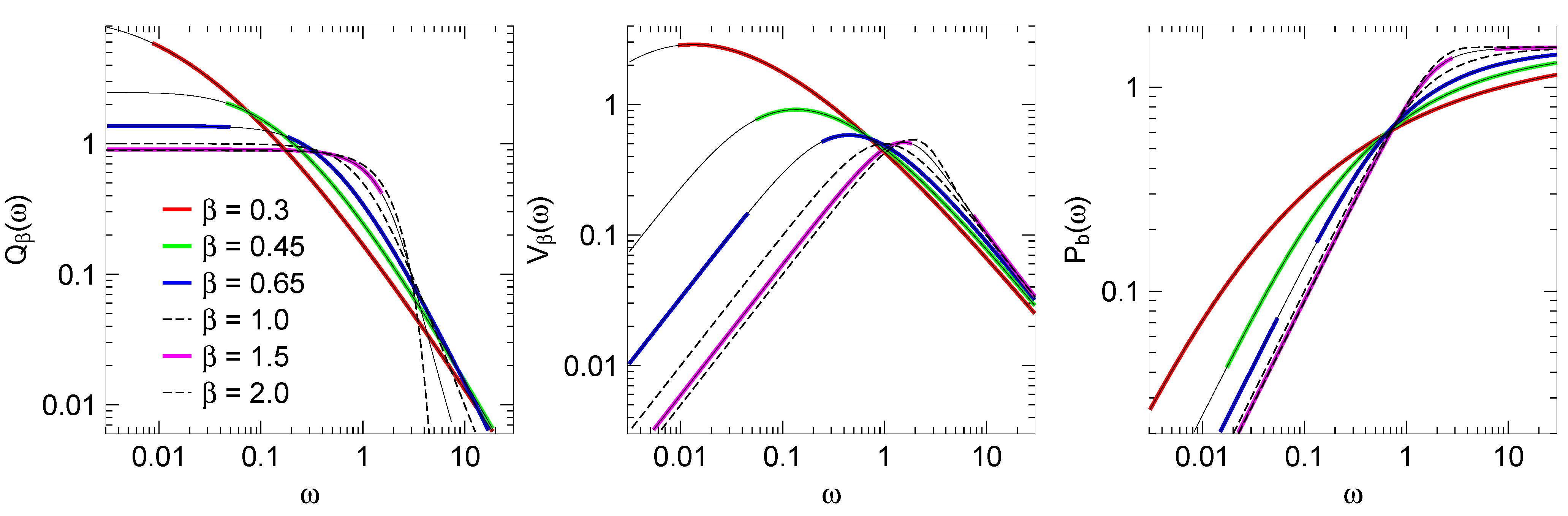
4. Series Expansions

4.1. Small-ω Expansion

For small and for large values of ω, F β ( ω ) can be determined from series expansions [1,2,26,27,28]. For small ω, we expand exp ( i ω t ) in Equation (4), substitute x = t β , and use the defining equation of the gamma function,
0 d x x μ - 1 e - x = : Γ ( μ )
to one obtain the Taylor series (in [28] traced back to Cauchy 1853):
F β ( ω ) = 1 β k = 0 A k ( i ω ) k
with
A k : = Γ ( ( k + 1 ) / β ) Γ ( k + 1 )
Separating real and imaginary parts, we get
Q β ( ω ) = 1 β k = 0 ( - 1 ) k A 2 k ω 2 k V β ( ω ) = 1 β k = 0 ( - 1 ) k A 2 k + 1 ω 2 k + 1
The expansion of P β is obtained most easily by integrating that of Q β ,
P β ( ω ) = 1 β k = 0 ( - 1 ) k A 2 k 2 k + 1 ω 2 k + 1
The expansions of Q β ( ω ) , V β ( ω ) , and P β ( ω ) shall be summarized as
Y = k = 0 ( - 1 ) k A 2 k + κ ( 2 k + 1 ) μ ω 2 k + κ + μ
with switches
κ , μ : = 0 , 0 for Q 1 , 0 for V 0 , 1 for P
All these series are useful only for small ω; otherwise large alternating terms prevent efficient summation. For β 1 , they converge for all values of ω. For β < 1 , they are asymptotic expansions, which means [32,33] they diverge, but when truncated at the right place they nevertheless provide useful approximations.

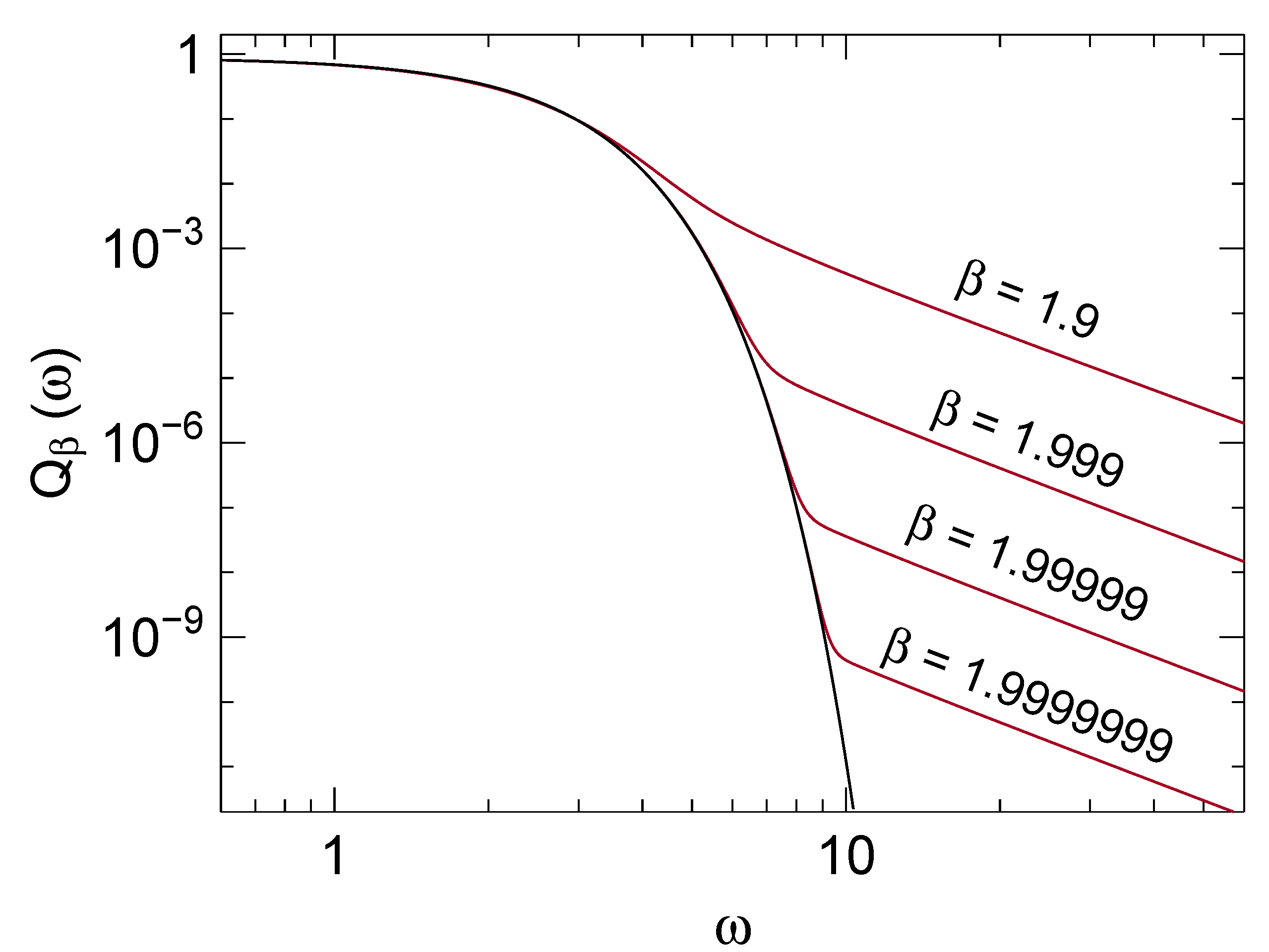
4.2. Large-ω Expansion

A complementary series expansion for large ω can be derived by expanding the exp ( - t β ) term in Equation (4). Using
0 d t t μ - 1 e i ω t = Γ ( μ ) ω μ e i μ π / 2
one obtains a series in powers of ω - β (in [28] attributed to Wintner 1941 [34]):
F β ( ω ) = i k = 0 ( - 1 ) k e ( ) i k β π / 2 B k ω - k β - 1
with
B k : = Γ ( k β + 1 ) Γ ( k + 1 )
Separating real and imaginary parts,
Q β ( ω ) = k = 1 ( - 1 ) k - 1 sin ( k β π / 2 ) B k ω - k β - 1 V β ( ω ) = k = 0 ( - 1 ) k cos ( k β π / 2 ) B k ω - k β - 1
Instead of P β , we compute its complement
P ¯ β ( ω ) : = P β ( ) - P β ( ω )
The limit P β ( ) = π / 2 is obtained most easily through Equation (6). Integration of Equation (21)
P ¯ β ( ω ) = ω d ω Q β ( ω )
yields
P ¯ β ( ω ) = k = 1 ( - 1 ) k - 1 sin ( k β π / 2 ) B k k β ω - k β
The expansions of Q β ( ω ) , V β ( ω ) , and P ¯ β ( ω ) shall be summarized as
Y = ( - 1 ) 1 - κ k = 1 - κ ( - 1 ) k sin ( k β + κ ) π 2 u k
with
u k : = B k ( k β ) - μ ω μ - 1 - k β
and with switches κ, μ as defined in Equation (17). To improve the numeric accuracy of the sine term in Equation (25) for β 2 , the complementary exponent β ¯ : = 2 - β is introduced so that ( - 1 ) 1 + k sin ( k β π / 2 ) can be replaced by sin ( k β ¯ π / 2 ) .
For β 1 , these series converge for all ω 0 ; for β > 1 , they are asymptotic expansions. This is just complementary to the small-ω expansion.

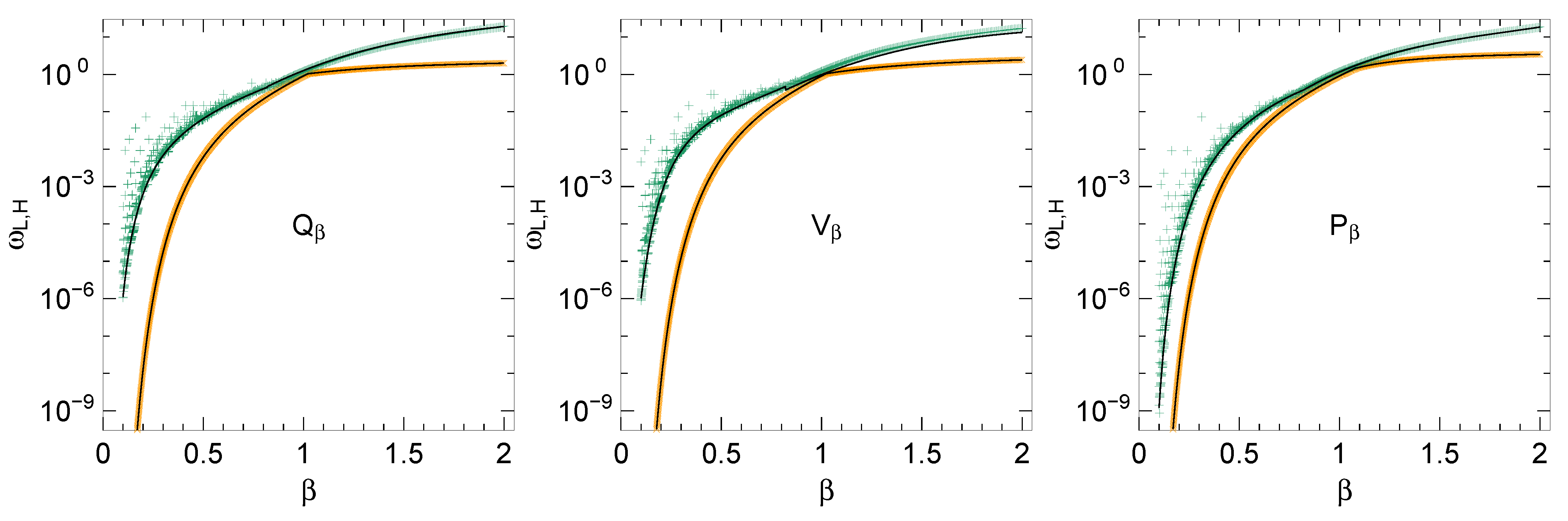
4.3. Cross-Over Frequencies

The leading-order terms in Equations (14) and (21) are power-laws in ω. In a plot of ln Q β or ln V β versus ln ω , these power-law asymptotes are straight lines that intersect at
ω Q : = β Γ ( 1 + β ) sin ( β π / 2 ) Γ ( 1 / β ) 1 / ( 1 + β )
and
ω V : = β Γ ( 2 / β ) 1 / 2
For β 0 , both cross-over frequencies go rapidly to zero, with a leading singularity
ω Q , V β 1 / β
This explains why the limiting case β 0 has no practical importance, and it also explains why previously published tables [1] of Q β ( ω ) and V β ( ω ) are useless for small exponents β 0 . 3 : As these tables employ the same linear ω grid for all β, for small β they only cover the asymptotic large-ω power-law regime, and not the nontrivial cross-over regime for which alone a table would be needed.
For β 2 , ω Q goes to zero because of the sine term in Equation (27). This regime, probably of little practical importance, will be dealt with in Section 5.6.

4.4. Error Bounds and Algorithm

The series (16) and (25) shall be approximated by finite sums
Y n = k = k 0 n - 1 y k
To control the accuracy of this approximation, we need an analytical bound r n for the truncation error
Δ tr Y n : = | Y n - Y | r n
For the small-ω expansion, in Appendix C the bound r n = | y n | is derived: The truncation error is not larger than the first neglected term. For the large-ω expansion, a bound is derived in Appendix D:
r n = ( sin ϕ ) - n β - 1 u n
with the auxiliary variable
ϕ : = π / 2 i f β 1 π / ( 2 β ) i f β > 1
and with u n as defined in Equation (26).
To avoid cancellation, the sum (30) is computed using an extended floating-point precision ϵ, as described in Section 1. This ensures an upper bound for the total floating-point error of
Δ fp Y n k = k 0 n - 1 ϵ | y k | = ϵ Z n
with the sum of absolute values
Z n : = k = k 0 n - 1 | y k |
Y n is requested to approximate Y with a relative accuracy of δ,
( Δ fp + Δ tr ) Y n δ · Y n
which is assured if
ϵ Z n + r n Y n δ
This leads to the following algorithm:
For each n = k 0 + 1 , k 0 + 2 , , compute y n - 1 , Y n , Z n , and r n . Terminate and return Y n if Equation (37) is fulfilled. Terminate and return an error code if one of the following conditions is met:
(i) y k is excessively large (approaching the largest floating-point number);
(ii) y k is excessively small (approaching the smallest normalized floating-point number);
(iii) ϵ Z n / Y n δ : alternating terms have cancelled each other to an extent that floating-point errors may exceed δ;
(iv) this is an asymptotic expansion and r k + 1 > r k ;
(v) a preset limit n = n lim is reached.
Since y k and r k require in part the same computations, the common factor u k is computed ahead to avoid the repetition of gamma function evaluations and other costly operations. For the small-ω expansion, we have just r k = u k and y k = ( - 1 ) k u k ; for the large-ω expansion, u k is defined in (26).

4.5. Application Domains

Let ω L ( β ) be the smallest ω at given β for which the small-ω algorithm returns an error code. Similarly, ω H ( β ) is the largest ω for which the large-ω expansion fails. Figure 2 shows these six limits, determined by a simple script (kww_findlims, cf. Section 6.4), as function of β. Results for Q V, and P are very similar. For β < 1 , the ω H ( β ) fluctuate strongly, due to the trigonometric factor in Equation (25).
For later use (Section 6.3), the ω L , H ( β ) are approximated by simple functions ω ˜ L , H ( β ) , defined piecewise after dividing the β-range [ 0 . 1 , 2 ] in two or three sections. Typically, within one section, ω ˜ L , H ( β ) is an exponential of a rational function with three or four parameters. Details can be found in the source kww.c where the fit results are hardcoded. For the fluctuating data at β < 1 , ω ˜ H ( β ) approximates the lower bound rather than the full data set.
Figure 2. Frequency limits for the series expansions for a required accuracy δ = 2 × 10 - 16 and a machine precision ϵ = 1 × 10 - 19 . Orange points represent ω L , green points ω H . Black lines show the piecewise fits that are hardcoded in libkww to decide whether a series expansion is tried or whether numeric integration is used from the outset.
Algorithms 05 00604 g002

5. Numeric Integration

5.1. Notation

The definitions (5) and (7) of Q β , V β , and P β can be summarized as
Y = 0 d t sin ( ω t + ν π ) g ( t )
with
g ( t ) : = t - μ f β ( t )
and
ν , μ : = 1 / 2 , 0 for Q 0 , 0 for V 0 , 1 for P

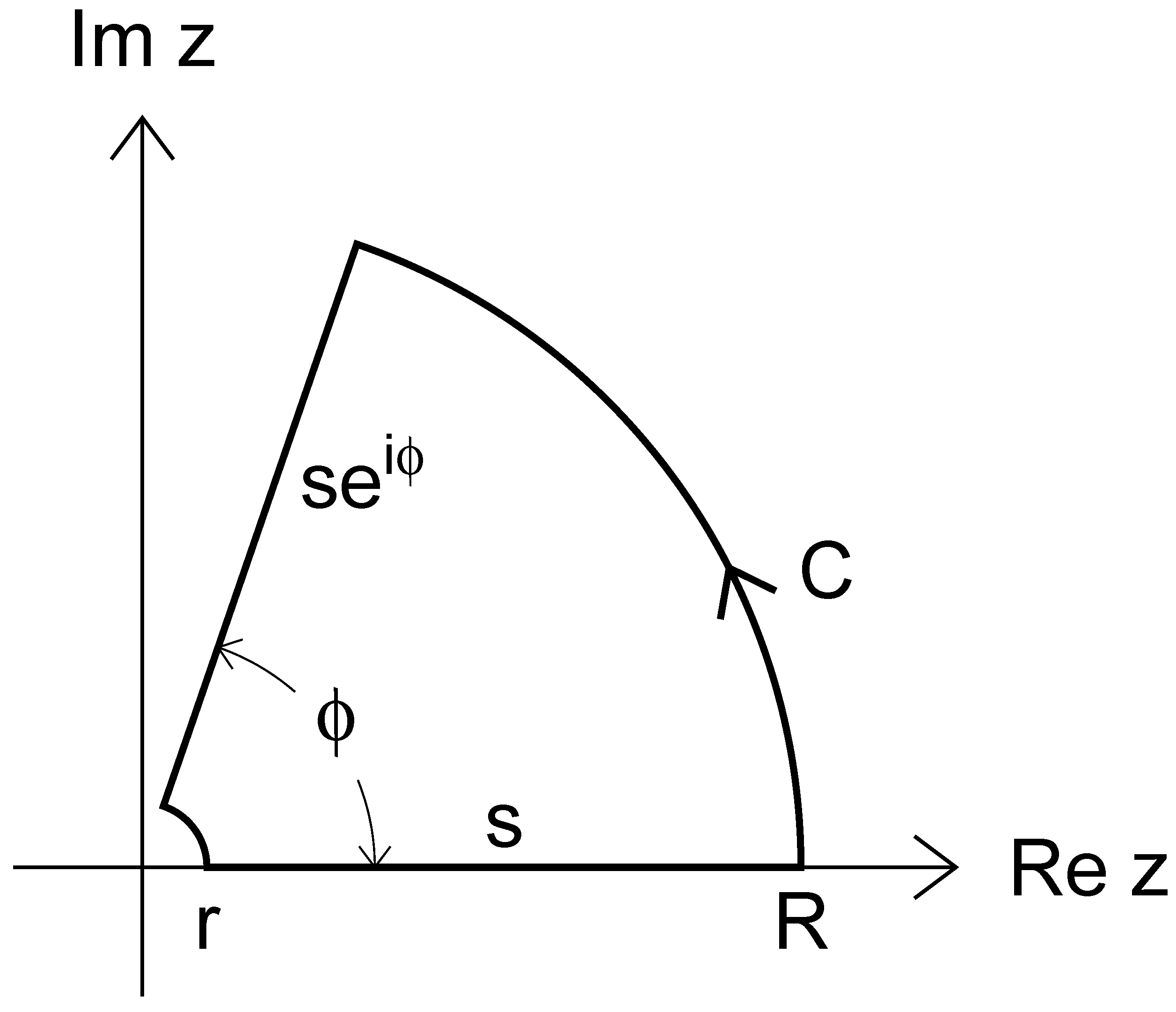
5.2. Integrating on a Double-exponential Grid

Popular approaches to calculate numeric Fourier transforms include straightforward fast Fourier transform, and Tuck’s simple “Filon-trapezoidal” rule [35]. Both methods evaluate the Fourier integrand on an equidistant grid t k = k Δ t . The Filon rule optimizes the weight of the grid points.
In our application, especially for small β, the decay of g ( t ) extends over several decades. To limit the number of grid points that must be taken into account, it is customary to use a decimation algorithm. A more efficient and perhaps even simpler alternative is the double-exponential transformation. It was first proposed by Takahasi and Mori in 1974 for the efficient evaluation of integrals with end-point singularities [36,37]. Afterwards, it was adapted to oscillatory functions by Ooura and Mori [38,39]. The key idea is to choose grid points t k close to the zeros of the sine function in Equation (38).
A double-exponential transformation is a monotonous function ϕ ( x ) that satisfies
ϕ ( x - ) 0
ϕ ( x - ) 0   double   exponentially
ϕ ( x + ) x   double   exponentially
This transformation shall now be applied to the time variable in the Fourier integral Equation (38):
t = π ω ϕ ( k - ν )
yielding
Y = π ω - d k ϕ ( k - ν ) sin ( π ( ϕ ( k - ν ) + ν ) ) g π ϕ ( k - ν ) ω
It is convenient to abbreviate
a k : = π ϕ ( k - ν )
b k : = ϕ ( k - ν ) sin ( π ( ϕ ( k - ν ) + ν ) )
Y ˜ : = ω π Y
The integral Equation (45) shall now be approximated by a sum, using the trapezoidal rule with stepwidth 1:
Y ˜ = k = - + b k g a k ω + Δ di Y ˜
where the last term is the discretization error, to be discussed below (Section 5.4). As a second approximation, we truncate the summation at ± N ,
Y ˜ = k = - N + N b k g a k ω + Δ di Y ˜ + Δ tr Y ˜
where the new term is the truncation error, also discussed below. This sum is used in libkww to compute the KWW function at intermediate frequencies. Since a k and b k do not depend on β and ω, they must be generated only once, which greatly accelerates repeated evaluations of Equation (50).
In practice, (50) can be well approximated with relatively small N. For k - , condition (42) ensures that b k goes double exponentially to 0. For k + , condition (43) makes the argument of the sine function in Equation (47) tend towards π k . If N is integer, then all k are integer as well, and the sine can be expanded around sin ( π k ) = 0 . In consequence, | b k | goes double exponentially to 0.

5.3. Choosing a Double-exponential Transform

To proceed, the double-exponential transformation must be specified. All ϕ considered by Ooura and Mori [39] have the form
ϕ ( x ) = x 1 - exp - η ( x )
Inserting this in Equation (47), the sine term can be recast to make b k robust for large k:
b k = ϕ ( k - ν ) ( - 1 ) k sin π ( k - ν ) e η ( k - ν ) - 1
Next, the function η shall be chosen. It must fulfill the conditions
η ( x - ) -   exponentially
η ( 0 ) = 0
η ( x + )   exponentially
Condition (54) guarantees that numerator and denominator of Equation (51) have a zero at the same location x = 0 . This singularity is removable; the values
ϕ ( 0 ) = 1 η ( 0 ) , ϕ ( 0 ) = 1 2 1 - η ( 0 ) η ( 0 ) 2
are needed to compute a 0 and b 0 for ν = 0 . Originally, Ooura and Mori [38] had proposed
η OM ( k ) : = 2 p sinh ( h k )
with p = 3 or p = π . The parameter h controls the mesh width in t; it will be determined below in Equation (65). In a later study, Ooura and Mori suggested a more complicated function η ( x ) that copes better with singularities near the real axis [39]. Since our kernel g ( t ) has no such singularities, we stay with the simple form Equation (57), extending it however by a linear term that decelerates the exponential asymptote at equal η ( 0 ) :
η ( k ) : = 2 p sinh ( h k ) + 2 q h k
Given the poor signal-to-noise ratio δ / ϵ , it was not possible to find one parameterization for the entire β , ω domain not covered by series expansions. Therefore, distinct sets of a k and b k are precomputed for five β ranges, using the parameter set shown in Table 1.
Table 1. Hand-optimized parameters p, q for different β ranges, for use in the kernel η (58) of the double-exponential transform ϕ (51).
βpq
0.1…0.151.80.2
0.15…0.251.60.4
0.25 …1.01.40.6
1.0 …1.751.00.2
1.75 …1.950.750.2
1.95 …20.150.4

5.4. Truncation Error and Mesh Width

There are three sources of errors: Floating-point cancellation, discretization, and truncation. A bound for the floating-point error Δ fp Y ˜ can be estimated as in Equation (34). The discretization error will be controlled by iterative refinement of the grid (Section 5.5).
Truncation errors arise from the introduction of finite summation limits in Equation (50). The truncation error at the lower summation limit is
Δ tr - Y ˜ = - - N d k ϕ ( k ) cos ( ) g ( ) < - - N d k | ϕ ( k ) |
Provided ϕ ( k ) does not change its sign for k < - N , the absolute-value operator can be omitted, and the integral becomes trivial, yielding
Δ tr - Y ˜ < ϕ ( - N ) N e η ( - N )
To obtain a bound for the upper truncation error, we start from the trapezoidal sum:
Δ tr + Y ˜ k = N + 1 b k g ( )
Using Equation (52),
Δ tr + Y ˜ < k = N + 1 + ν ϕ ( k ) π N e η ( k ) - 1 k = N + 1 π N e - η ( k )
The summands decay faster than in a geometric series so that
Δ tr + Y ˜ < π N e - η ( + N )
similar to Equation (60). Altogether, the truncation error decreases double exponentially with increasing N. Therefore we can request at very little cost a safety factor of m = 10 or more in the error bound,
Δ tr Y ˜ / Y ˜ < δ / m
which ensures that truncation contributes almost nothing to the overall error. For the same reason we must not care about the non-strict (≲) estimates in Equations (60) and (62).
To make use of Equation (64), we need a lower bound for Y ˜ . From the data shown in Figure 2, we can infer that the lowest Y ˜ that needs to be computed numerically is at β = 0 . 1 , Y = V ; its value is little above Y ˜ 0 : = 2 · 10 - 20 . The choice Equation (58) ensures the asymptotic behavior η ( x ) ± q e h x for x ± . Thence Equation (64) is satisfied by
h = 1 N ln 1 q ln ( π + 1 ) m N δ Y ˜ 0

5.5. Iterative Integration

The numeric integration is performed by computing the trapezoidal sum (50) in iterations n = 0 , 1 , with increasing mesh size N n and decreasing steps h n ,
Y ˜ n : = k = - N n N n b k n g a k n ω
In libkww, the simple iteration scheme
N n = 2 n N 0
is used, and h n is set according to Equation (65).
To estimate the floating-point error, we also need the sum of absolute terms
T ˜ n : = k = - N n N n | b k n | g a k n ω
The discretization error is estimated by comparing the present with the previous result,
Δ di Y ˜ Y ˜ n - Y ˜ n - 1
The non-strict less-than symbol in this equation is the weakest point of this entire work, opening the door for uncontrolled errors. We therefore depend on heuristic evidence that discretization errors almost never exceed a few δ (Section 6.4). The success criterion is thus
Δ fp Y ˜ + Δ di Y ˜ ϵ T ˜ n + Y ˜ n - Y ˜ n - 1 δ Y ˜ n
If the latter inequality is fulfilled, the algorithm terminates and returns Y ˜ n . Otherwise, when n reaches a limit n lim , the iteration exits with an error code.

5.6. Special Case β 2

Figure 3 shows Q β ( ω ) for representative values of β. In the limit β = 2 , the cosine transform is just a Gaussian,
Q 2 ( ω ) = π 2 exp - ω 2 / 4
whereas for β 2 it has a power-law tail
Q 2 - β ¯ ( ω ) sin ( β ¯ π / 2 ) Γ ( 2 - β ¯ ) ω - 3 + β ¯ for   ω 1
This qualitative change is also evident from the high ω expansion (21), which becomes useless at β = 2 where sin ( k β π / 2 ) = 0 for all k. All this is not a problem, but in the ω range between the two series expansions, the numeric quadrature fails to reach the required accuracy because of cancellation. This problem can be remediated to a certain degree by transforming not f β ( t ) but the difference f β ( t ) - f 2 ( t ) . The result is then added to the analytic transform Q 2 ( ω ) . In our implementation, this is done for 1 . 75 < β < 2 . Even then, for β > 1 . 9 the integration fails for some ω.
Figure 3. Red lines: Cosine transform Q β ( ω ) close to the Gaussian limit β 2 . Black line: Gaussian π / 4 exp ( - ω 2 / 4 ) .
Algorithms 05 00604 g003

6. Implementation

6.1. Download and Installation

Routines for the computation of Q β ( ω ) , V β ( ω ) and P β ( ω ) have been implemented in form of a small library libkww. In order to ensure maximum portability, the programming language C has been chosen. The source code is published under the terms of the GNU General Public License (GPL); other licenses can be negotiated when needed. The source distribution is available as a tar archive. Version 3.0 is deposited as supplementary material to this article. Updates can be found on our institute’s application server at http://apps.jcns.fz-juelich.de/kww; changes are documented in the file CHANGE_LOG, which is part of the source distribution.
The build procedure is automatized with GNU autotools; the distribution contains all files needed to build the library and some test programs with the standard command sequence ./configure, make, sudo make install. The source code resides in the subdirectory lib/. The build process normally produces a static and a dynamic version of the library libkww, and installs it to the appropriate location. Besides, a header file kww.h is copied to the appropriate include directory. Subdirectory test/ contains programs and scripts used for fine-tuning and testing. Subdirectory doc/ provides a manual page kww (3) in plain old documentation (POD) format. The tools pod2man and pod2html are required to translate it into Unix manual (*roff) and HTML formats.

6.2. Application Programming Interface, Error Handling

The application programming interface (API) for computing Q β ( ω ) , V β ( ω ) and P β ( ω ) can be summarized as follows:
#include <kww.h> double kwwc (double omega, double beta);
double kwws (double omega, double beta);
double kwwp (double omega, double beta);
The letters c and s stand for cosine and sine transform, respectively; p stands for the primitive of the cosine transform.
If β is outside the allowed range 0 . 1 β 2 , an error message is written to stderr, and exit is called with errno EDOM. For the cosine transform, the range 1 . 9 < β < 2 . 0 is allowed but not supported: failures of the numeric integration in this range will not be considered bugs. If the numeric integration fails in the non-supported range, kwwc simply returns 0.
A failure of the numeric integration in the supported β range is considered a bug. An error message is written to stderr, and exit is called with errno ENOSYS. Such failures should be reported to the author who will try to fix them by fine tuning the double exponential transform, or by slightly increasing δ. If it turns out that the insufficient signal-to-noise ratio of long double versus double does not permit to fully exclude occasional failures at isolated ω , β , then the error handling will be changed in future releases. At any moment, the man page provides the authoritative documentation.

6.3. Low-level Functions

In a few special cases ( ω = 0 , or β = 2 for the cosine transform), the analytically known return value is computed immediately. If ω < 0 , the absolute value is taken; for the kwws and kwwp, a flag is set so that the functions can ultimately return Y ( ω ) = ± Y ( | ω | ) for ω 0 . In the following, as everywhere else in this text, we consider only ω > 0 .
The domain limits ω ˜ L , H are hardcoded in functions
double kwwc_lim_low( double b ); double kwwc_lim_hig( double b );
and similar for kwws and kwwp. If ω ω ˜ L ( β ) or ω ω ˜ H ( β ) , the appropriate series expansion is tried. If it returns an error code (return value below 0) the computation falls back to numeric integration. If ω lies between ω ˜ L and ω ˜ H , the numeric integration is invoked from the outset.
Series expansions and numeric integration are implemented by the functions
double kwwc_low( double w, double b );
double kwwc_mid( double w, double b );
double kwwc_hig( double w, double b );
and similar for kwws and kwwp. For test purposes, these low-level functions can also be called directly.
Since the algorithms for all three functions are very similar, they are implemented jointly: The above functions are no more than thin wrappers around the core functions
double kww__low( double w, double b, int kappa, int mu);
double kww__mid( double w, double b, int kind, int mu);
double kww__hig( double w, double b, int kappa, int mu);
where the actual computations are carried out, following the algorithms described above (Section 4.4, Section 5.5), with kind = 1 - 2 ν .

6.4. Diagnostic Variables and Test Programs

For optimizing and testing the program, it is important to know which algorithm is chosen for given ω , β , and how many terms need to be summed. This information is provided by two global variables in the source file kww.c. Programs linked with libkww can access them using extern declarations:
extern int kww_algorithm; extern int kww_num_of_terms;
The variable kww_algorithm is set to 1, 2, or 3, to indicate whether the low-ω expansion, the numeric integration, or the high-ω expansion has been used. The variable kww_num_of_terms counts the evaluations of f β .
The test program runkww (source code runkww.c in directory test/) allows to call the high-level functions of Section 6.2 and the low-level functions of Section 6.3 from the command line. If the program is called without arguments, it prints a help text. Besides the function values Q β ( ω ) or V β ( ω ) , runkww also prints the diagnostic variables described above.
The script kww_findlims.rb, written in the Ruby programming language, uses bisection to determine the limits ω L , H where the series expansion first fails.
The program kww_countterms tests the numeric integration within a hardcoded β range and for ω within the limits ω ˜ L , H , and prints the average number of evaluations of f β . It has been used to optimize the parameters p and q of the kernel η of the double-exponential transform ϕ (Section 5.3).
The script kww_checks.rb performs scans in ω at fixed β, or vice versa, and detects points where the used algorithm or the number of function evaluations has changed. It then checks the continuity of Y = Q , V , P across this border. Results of numerous test runs confirm that violations of monotonicity are extremely rare and never exceed a few δ.

Acknowledgments

I thank S. Busch, T. Franosch, D. Korolkov, and T. Voigtmann for feedback on early manuscript versions, and W. Van Herck for carefully checking the final text.

References

  1. Dishon, M.; Weiss, G.H.; Bendler, J.T. Stable Law Densities and Linear Relaxation Phenomena. J. Res. N. B. S 1985, 90, 27–40. [Google Scholar] [CrossRef]
  2. Chung, S.H.; Stevens, J.R. Time-dependent correlation and the evaluation of the stretched exponential or Kohlrausch-Williams-Watts function. Am. J. Phys. 1991, 59, 1024–1029. [Google Scholar] [CrossRef]
  3. Cardona, M.; Chamberlin, R.V.; Marx, W. The history of the stretched exponential function. Ann. Phys. (Leipzig) 2007, 16, 842–845. [Google Scholar] [CrossRef]
  4. Böhmer, R.; Ngai, K.L.; Angell, C.A.; Plazek, D.J. Nonexponential relaxations in strong and fragile glass formers. J. Chem. Phys. 1993, 99, 4201–4210. [Google Scholar] [CrossRef]
  5. Phillips, J.C. Anomalous glass transitions and stretched exponential relaxation in fused salts and polar organic compounds. Phys. Rev. E 1996, 53, 1732–1739. [Google Scholar] [CrossRef]
  6. Ngai, K.L. Relaxation and Diffusion in Complex Systems; Springer: New York, NY, USA, 2011. [Google Scholar]
  7. Wiebel, S.; Wuttke, J. Structural relaxation and mode coupling in a non-glassforming liquid: depolarized light scattering in benzene. New J. Phys. 2002, 4, 56. [Google Scholar] [CrossRef]
  8. Torre, R.; Bartolini, P.; Righini, R. Structural relaxation in supercooled water by time-resolved spectroscopy. Nature 2004, 428, 296–299. [Google Scholar] [CrossRef] [PubMed]
  9. Turton, D.A.; Wynne, K. Crossover from Stretched to Compressed Exponential Relaxations in a Polymer-Based Sponge Phase. J. Chem. Phys. 2009, 131, 201101. [Google Scholar] [CrossRef] [PubMed] [Green Version]
  10. Berberan-Santos, M.N.; Bodunov, E.N.; Valeur, B. Mathematical functions for the analysis of luminescence decays with underlying distributions 1. Kohlrausch decay function (stretched exponential). Chem. Phys. 2005, 315, 171–182. [Google Scholar]
  11. Phillies, G.D.J.; Peczak, P. The ubiquity of stretched-exponential forms in polymer dynamics. Macromolecules 2002, 21, 214–220. [Google Scholar] [CrossRef]
  12. Nakamura, H.K.; Sasai, M.; Takano, M. Scrutinizing the squeezed exponential kinetics observed in the folding simulation of an off-lattice Go-like protein model. Chem. Phys. 2004, 307, 259–267. [Google Scholar] [CrossRef]
  13. Falus, P.; Borthwick, M.A.; Narayanan, S.; Sandy, A.R.; Mochrie, S.G.J. Crossover from Stretched to Compressed Exponential Relaxations in a Polymer-Based Sponge Phase. Phys. Rev. Lett. 2006, 97, 066102. [Google Scholar] [CrossRef] [PubMed]
  14. Hamm, P.; Helbing, J.; Bredenbeck, J. Stretched versus compressed exponential kinetics in α-helix folding. Chem. Phys. 2006, 323, 54–65. [Google Scholar] [CrossRef]
  15. Xi, H.; Franzen, S.; Guzman, J.I.; Mao, S. Degradation of magnetic tunneling junctions caused by pinhole formation and growth. J. Magn. Magn. Mat. 2007, 319, 60–63. [Google Scholar] [CrossRef]
  16. Laherrère, J.; Sournette, D. Stretched exponential distributions in nature and economy: “fat tails” with characteristic scales. Eur. Phys. J. B 1998, 2, 525–539. [Google Scholar] [CrossRef]
  17. Davies, J.A. The individual success of musicians, like that of physicists, follows a stretched exponential distribution. Eur. Phys. J. B 2002, 27, 445–447. [Google Scholar] [CrossRef]
  18. Sinha, S.; Raghavendra, S. Hollywood blockbusters and long-tailed distributions—An empirical study of the popularity of movies. Eur. Phys. J. B 2004, 42, 293–296. [Google Scholar] [CrossRef]
  19. Götze, W.; Sjögren, L. The glass transition singularity. Z. Phys. B 1987, 65, 415–427. [Google Scholar] [CrossRef]
  20. Fuchs, M. The Kohlrausch law as a limit solution to mode coupling equations. J. Non-Cryst. Solids 1994, 172–174, 241–247. [Google Scholar] [CrossRef]
  21. Metzler, R.; Klafter, J. From stretched exponential to inverse power-law: fractional dynamics, Cole¨CCole relaxation processes, and beyond. J. Non-Cryst. Solids 2002, 305, 81–87. [Google Scholar] [CrossRef]
  22. Götze, W. Complex Dynamics of Glass-Forming Liquids. A Mode-Coupling Theory; Oxford University Press: Oxford, UK, 2009. [Google Scholar]
  23. Anderssen, R.S.; Husain, S.A.; Loy, R.J. The Kohlrausch function: properties and applications. ANZIAM J. 2004, 45, C800–C861. [Google Scholar]
  24. Husain, S.A.; Anderssen, R.S. Modelling the relaxation modulus of linear viscoelasticity using Kohlrausch functions. J. Non-Newton. Fluid Mech. 2005, 125, 159–170. [Google Scholar] [CrossRef]
  25. Williams, G.; Watts, D.C. Non-symmetrical dielectric relaxation behaviour arising from a simple empirical decay function. Trans. Faraday Soc. 1970, 66, 80–85. [Google Scholar] [CrossRef]
  26. Williams, G.; Watts, D.C.; Dev, S.B.; North, A.M. Further considerations of non symmetrical dielectric relaxation behaviour arising from a simple empirical decay function. Trans. Faraday Soc. 1971, 67, 1323–1335. [Google Scholar] [CrossRef]
  27. Lindsey, C.P.; Patterson, G.D. Detailed comparison of the Williams¨C-Watts and Cole-¨CDavidson functions. J. Chem. Phys. 1980, 73, 3348–3347. [Google Scholar] [CrossRef]
  28. Montroll, E.W.; Bendler, J.T. On Lévy (or stable) distributions and the Williams-Watts model of dielectric relaxation. J. Stat. Phys. 1984, 34, 129–162. [Google Scholar] [CrossRef]
  29. Macdonald, J.R. Accurate fitting of immittance spectroscopy frequency-response data using the stretched exponential model. J. Non-Cryst. Solids 1997, 212, 95–116. [Google Scholar] [CrossRef]
  30. Alvarez, F.; Alegría, A.; Colmenero, J. Relationship between the time-domain Kohlrausch-Williams-Watts and frequency-domain Havriliak-Negami relaxation functions. Phys. Rev. B 1991, 44, 7306–7312. [Google Scholar] [CrossRef]
  31. Alvarez, F.; Alegría, A.; Colmenero, J. Interconnection between frequency-domain Havriliak-Negami and time-domain Kohlrausch-Williams-Watts relaxation functions. Phys. Rev. B 1993, 47, 125–130. [Google Scholar] [CrossRef]
  32. Copson, E.T. Asymptotic Expansions; Cambridge University Press: Cambridge, UK, 1965. [Google Scholar]
  33. Bleistein, N.; Handelsman, R.A. Asymptotic Expansion of Integrals; Dover Publications: London, UK, 1986. [Google Scholar]
  34. Wintner, A. The singularities of Cauchy¡¯s distributions. Duke Math. J. 1941, 8, 678–681. [Google Scholar] [CrossRef]
  35. Tuck, E.O. A Simple “Filon-trapezoidal” rule. Math. Comput. 1967, 21, 239–241. [Google Scholar] [CrossRef]
  36. Mori, M.; Sugihara, M. The double-exponential transformation in numerical analysis. J. Comp. Appl. Math. 2001, 127, 287–296. [Google Scholar] [CrossRef]
  37. Mori, M. Discovery of the double exponential transformation and its developments. Publ. RIMS, Kyoto Univ. 2005, 41, 897–935. [Google Scholar] [CrossRef]
  38. Ooura, T.; Mori, M. The double exponential formula for oscillatory functions over the half infinite interval. J. Comp. Appl. Math. 1991, 38, 353–360. [Google Scholar] [CrossRef]
  39. Ooura, T.; Mori, M. A robust double exponential formula for Fourier-type integrals. J. Comp. Appl. Math. 1999, 112, 229–241. [Google Scholar] [CrossRef]
  40. Kubo, R. The fluctuation-dissipation theorem. Rep. Progr. Phys. 1966, 29, 255–284. [Google Scholar] [CrossRef]
  41. Doster, W.; Busch, S.; Gaspar, A.M.; Appavou, M.S.; Wuttke, J.; Scheer, H. Dynamical transition of protein-hydration water. Phys. Rev. Lett. 2010, 104, 098101. [Google Scholar] [CrossRef] [PubMed]
  42. Scarborough, J.B. Numerical Mathematical Analysis; John Hopkins Press: Baltimore, ML, USA, 1930; The statement about usual truncation errors in asymptotic series is on p. 158 of the 2nd edition (1950), and on p. 164 of the 5th edition (1962). [Google Scholar]
  43. Charlier, C.L. Die Mechanik des Himmels. Zweiter Band; Veit & Comp.: Leipzig, Germany, 1907. [Google Scholar]
  44. NIST Digital Library of Mathematical Functions. Available online: http://dlmf.nist.gov, 7.2.5 and 7.7.3 (accessed on 20 November 2012).
  45. GNU Scientific Library, version GSL-1.15 of 6 May 2011, chapter 7.9. Available online: http://www.gnu.org/software/gsl/manual/html_node/Dawson-Function.html (accessed on 20 November 2012).

Appendix

A. Description of Relaxation in Time and Frequency

The use of the Fourier transform to describe dynamic susceptibilities and scattering experiments has its foundations in linear response theory. In this appendix, the relations between response functions, relaxation functions, susceptibilities, correlation functions, and scattering laws shall be briefly summarized.
The linear response B ( t ) to a perturbation A ( t ) can be written as
B ( t ) = - t d t R ( t - t ) A ( t )
Consider first the momentary perturbation A ( t ) = δ ( t ) . The response is B ( t ) = R ( t ) . Therefore, the memory kernel R is identified as the response function.
Consider next a perturbation A ( t ) = e η t Θ ( - t ) that is slowly switched on and suddenly switched off (Θ is the Heaviside step function, η is sent to 0 + at the end of the calculation). For t > 0 , one obtains B ( t ) = Φ ( t ) where Φ is the negative primitive of the response function
R ( t ) = - t Φ ( t )
Since Φ describes the time evolution after an external perturbation has been switched off, it is called the relaxation function. Kohlrausch’s stretched exponential function is a frequently used approximation for Φ ( t ) .
Consider finally a periodic perturbation that is switched on adiabatically, A ( t ) = exp ( - i ω t + η t ) , implying again the limit η 0 + . Introducing the dynamic susceptibility
χ ( ω ) : = 0 d t e i ( ω + i η ) t R ( t )
the response can be written B ( t ) = χ ( ω ) A ( t ) . To avoid the differentiation (74) in the integrand, it is more convenient to transform the relaxation function,
F ( ω ) : = 0 d t e i ω t Φ ( t )
This is Equation (4), the starting point of the present work.
Partial integration yields a simple relation between χ and F:
χ ( ω ) = Φ ( 0 ) + i ω F ( ω )
In consequence, the imaginary part of the susceptibility, which typically describes the loss peak in a spectroscopic experiment, is given by the real part of the Fourier transform of the relaxation function, I m η = ω R e F ( ω ) .
Up to this point, the only physical input has been Equation (73). To make a connection with correlation functions, more substantial input is needed. Using the full apparatus of statistical mechanics (Poisson brackets, Liouville equation, Boltzmann distribution, Yvon’s theorem), it is found [40] that for classical systems
A ( t ) B ( 0 ) = k B T Φ ( t )
Pair correlation functions are typically measured in scattering experiments. For instance, inelastic neutron scattering at wavenumber q measures the scattering law S ( q , ω ) , which is the Fourier transform of the density correlation function,
S ( q , ω ) = 1 2 π - d t e i ω t ρ ( q , t ) * ρ ( q , 0 )
In contrast to Equations (4) and (75), this is a normal, two-sided Fourier transform. If we let ρ ( q , t ) * ρ ( q , 0 ) = Φ q ( t ) , then the scattering law S ( q , ω ) is
S ( q , ω ) = 1 π Re F q ( ω )

B. Convolution with a Resolution Function

In an inelastic scattering experiment, the observed spectrum is usually well approximated as a convolution
S R ( ω ) = - + d ω R ( ω ) S ( ω - ω )
of the physical spectrum S with the instrumental resolution R. Since the observed spectrum and the observed resolution are both given as histograms on a discrete ω mesh, the convolution integral is normally computed as a sum
S R ( ω i ) j Δ ω j R ( ω j ) S ( ω i - ω j )
This is a reasonable approximation as long as both S and R vary slowly from one ω channel to the next. As for R, this condition should be of no concern: in a well designed spectrometer, the channel width is chosen considerably smaller than the width of R.
However, the condition is not always fulfilled for S. Typical resolution functions have shapes between Gaussian and Lorentzian. If S is the Fourier transform of a stretched exponential with β < 1 , then the top of S can be much sharper than R, while the wings of S exceed those of R and cause noticeable quasielastic scattering (see, e.g., Figure 1 in [41]). In such a case, discrete values, especially the value S ( 0 ) , are not representative for entire ω channels. Instead of Equation (82), one needs to compute
S R ( ω i ) j R ( ω j ) - Δ ω j / 2 + Δ ω j / 2 d ω S ( ω i - ω j + ω )
The integration must not be carried out explicitly, since libkww provides a function kwwp that directly yields the primitive Equation (7) of Q β ( ω ) = π S ( ω ) , without passing through an evaluation of Q β . In consequence, fit programs should compute resolution-broadened Kohlrausch–Williams–Watts spectra as
π S R ( ω i ) j R ( ω j ) P ( ω i - ω j + Δ ω j / 2 ) - P ( ω i - ω j - Δ ω j / 2 )

C. Truncation Error in Small-ω Expansion

In this appendix, an upper bound for the truncation error of the small-ω expansion (14) is derived, improving upon a weaker and unproven estimate in [2]. We consider the cosine transform, and write the Taylor expansion with Lagrange remainder as
Q β ( ω ) = k = 0 n - 1 Q β ( k ) ( 0 ) ω k k ! + Q β ( n ) ( ξ ) ω n n !
with 0 ξ ω . Going back to the definitions (5) and (4), we have
Q β ( n ) ( ξ ) = Re F β ( n ) ( ξ ) F β ( n ) ( ξ ) = d n d ξ n 0 d t e i ξ t e - t β = 0 d t ( i t ) n e i ξ t e - t β 0 d t ( i t ) n e i ξ t e - t β = 0 d t t n e - t β = F β ( n ) ( 0 )
The coefficients Q β ( k ) ( 0 ) in Equation (85) are zero for odd k. Therefore we are free to choose n even. In this case, the upper bound derived in Equation (86) equals | Q β ( n ) ( 0 ) | so that we have
Q β ( n ) ( ξ ) ω n n ! Q β ( n ) ( 0 ) ω n n !
In conclusion, the truncation error is not larger than the first neglected term. This proof can be easily transcribed for the sine transform V β , and for the primitive of Q β ,
P β ( ω ) = k = 0 n - 1 Q β ( k ) ( 0 ) ω k + 1 ( k + 1 ) ! + Q β ( n ) ( ξ ) ω n + 1 ( n + 1 ) !

D. Truncation Error in Large-ω Expansion

In this appendix, an upper bound for the truncation error of the large-ω expansion (21) is derived. The following two unproven statements of [2] turn out to be wrong: (i) the most accurate results are obtained by truncating the summation before the smallest term; and (ii) the truncation error is less than twice the first neglected term.
We specialize again to the cosine transform Q β ( ω ) . If we choose β = 4 / 3 the oscillatory factor sin ( k β π / 2 ) in Equation (21) is zero for k = 3 . If the statements of [2] were correct, then we could stop the summation at k = 2 with a truncation error of zero for all values of ω. This is obviously wrong. A correct truncation criterion can only be based on the amplitudes B k ; it must disregard the oscillating prefactor sin ( k β π / 2 ) .
But even after omitting oscillatory factors the two statements are unfounded. In [2] they are underlaid by a reference to a specific page in a book on numerical analysis [42]. However, that page only says “the error committed is usually less than twice the first neglected term”, followed by a reference to a specific page in a 1907 book on Celestial Mechanics [43]. Going back to this source, we find a rigorous theorem, which however holds only under very restrictive conditions not fulfilled here.
Therefore we have to restart from scratch. We will simplify an argument of Wintner [34], and generalize it to cover not only the convergent case β 1 but also the asymptotic expansion for β > 1 .
Substituting s = ω t , the Fourier integral (4) takes the form
F β ( ω ) = ω - 1 0 d s exp i s - ω - β s β
We consider the cosine transform Q β ( ω ) = Re F β ( ω ) , which we rewrite as Q β ( ω ) = G ( ω - β ) / ω , introducing the functions
G ( x ) : = Re 0 d s γ ( s , x , 0 )
and
γ ( s , x , a ) : = s a exp i s - x s β
The Taylor expansion of G ( x ) , including the Lagrange remainder, reads
G ( x ) = k = 0 n - 1 G ( k ) ( 0 ) x k k ! + G ( n ) ( ξ ) x n n !
with 0 ξ x and
G ( k ) ( ξ ) = ( - 1 ) k Re 0 d s γ ( s , ξ , k β )
Now, we choose an integration path C in the complex plane consisting of two line segments, s and s e i ϕ , and two arcs, r e i φ and R e i φ , with 0 < r s R < and 0 φ ϕ π / 2 as shown in Figure 4. The integral of γ along this path is zero:
C d z γ ( z , x , a ) = 0
The contributions of the two arcs tend to 0 as r 0 and R . Hence the contributions of the two line segments have equal modulus. This allows us to obtain the following bounds:
G ( n ) ( ξ ) = ( - 1 ) n Re 0 d s γ ( s , ξ , n β ) 0 d s γ ( s , ξ , n β ) = 0 d s γ ( s e i ϕ , ξ , n β ) 0 d s γ ( s e i ϕ , ξ , n β ) = 0 d s s n β e i ϕ n β exp i s e i ϕ - ξ s β e i ϕ β = 0 d s s n β exp - s sin ϕ - ξ s β cos ( ϕ β )
At this point we choose ϕ as in Equation (33), which ensures cos ( ϕ β ) 0 . The bound
G ( n ) ( ξ ) 0 d s s n β exp - s sin ϕ
is independent of ξ. The integral is the same as in Equation (11). So we obtain bounds for the truncation error of G ( x )
G ( n ) ( ξ ) Γ ( n β + 1 ) ( sin ϕ ) n β + 1
and of Q β ( ω ) ,
r n = 1 ω Γ ( n β + 1 ) ( sin ϕ ) n β + 1 ω - n β n ! = B n ω - n β - 1 ( sin ϕ ) n β + 1 = u n ( sin ϕ ) n β + 1
By taking the imaginary part instead of the real part in Equation (90) the argument is readily adapted to the sine transform, and the same bound Equation (98) is obtained.
Figure 4. Integration path C in the complex plane used to compute an upper bound for G ( k ) ( ξ ) .
Algorithms 05 00604 g004
For the complementary primitive of Q, we make use of G ( 0 ) ( 0 ) to write
P ¯ β ( ω ) = ω d ω G ( ω - β ) ω = k = 1 n - 1 G ( k ) ( 0 ) ω - k β k ! k β + G ( n ) ( ξ ) ω - n β n ! n β
so that we can use the same bound for | G ( n ) ( ξ ) | as before in Equation (97). This yields a bound for the truncation error of P ¯ ,
r n = Γ ( n β + 1 ) ( sin ϕ ) n β + 1 ω - n β n ! n β = B n ω - n β n β ( sin ϕ ) n β + 1 = u n ( sin ϕ ) n β + 1

E. Analytic Solutions for β = 1 , 2

Just for reference, let us note the analytic solutions for β = 1 , 2 :
Q 1 ( ω ) = 1 π 1 1 + ω 2 , Q 2 ( ω ) = π 2 exp - ω 2 4 V 1 ( ω ) = 1 π ω 1 + ω 2 , V 2 ( ω ) = F Dawson ω 2 P 1 ( ω ) = 1 π arctan ( ω ) , P 2 ( ω ) = π 2 erf ω 2
with the Dawson’s integral [44]
F Dawson ( x ) : = exp ( - x 2 ) 0 x d t exp ( t 2 )
available in the GNU Scientific Library [45]. Analytic solutions also exist for β = 1 / 2 ; they involve Fresnel integrals and the Faddeeva function (complex complementary error function) [25].

