Dubins Traveling Salesman Problem with Neighborhoods: A Graph-Based Approach

Abstract

We study the problem of finding the minimum-length curvature constrained closed path through a set of regions in the plane. This problem is referred to as the Dubins Traveling Salesperson Problem with Neighborhoods (DTSPN). An algorithm is presented that uses sampling to cast this infinite dimensional combinatorial optimization problem as a Generalized Traveling Salesperson Problem (GTSP) with intersecting node sets. The GTSP is then converted to an Asymmetric Traveling Salesperson Problem (ATSP) through a series of graph transformations, thus allowing the use of existing approximation algorithms. This algorithm is shown to perform no worse than the best existing DTSPN algorithm and is shown to perform significantly better when the regions overlap. We report on the application of this algorithm to route an Unmanned Aerial Vehicle (UAV) equipped with a radio to collect data from sparsely deployed ground sensors in a field demonstration of autonomous detection, localization, and verification of multiple acoustic events.

1. Introduction

Research in the area of unmanned aerial vehicles (UAV) has evolved in recent years. There is rich literature covering various areas of autonomy including path planning, trajectory planning, task allocation, cooperation, sensing, and communications. As the mission objectives of UAVs have increased in complexity and importance, problems are starting to arise at the intersection of these disciplines. The Dubins Traveling Salesman Problem with Neighborhoods (DTSPN) combines the problem of path planning with trajectory planning while using neighborhoods to represent communication ranges or sensor footprints. In this problem the UAV simply needs to enter a region surrounding each objective waypoint.

1.1. Relevant Literature

The path planning problem seeks to determine the optimal sequence of waypoints to visit in order to meet certain mission objectives while minimizing costs, such as the total length of the mission [1,2]. Path planning problems typically rely on approximating the cost of the mission by the length of the solution to a Euclidean Traveling Salesman Problem (ETSP), where the cost to travel from one waypoint to the next is approximated by the Euclidean distance between the two waypoints. This approximation simplifies the overall optimization but may lead to UAV routes that are far from optimal because the aircraft kinematic constraints are not considered.

Another area of UAV research is trajectory planning, in which the goal given an initial and final waypoint pair is to determine the optimal control inputs to reach the final waypoint in minimum time given kinematic constraints of the aircraft. In 1957, Dubins showed that for an approximate model of aircraft dynamics, the optimal motion between a pair of waypoints can be chosen among six possible paths [3]. Similar results were proven later in [4] using tools from optimal control theory. In [5], the authors propose a means of choosing the optimal Dubins path without computing all six possible Dubins optimal paths.

A significant amount of research has gone into combining the problems of motion planning and path planning [6,7,8,9,10]. In these works, the dynamics of the UAV are taken into consideration by using the Dubins model when determining the optimal sequence of waypoints. This problem is typically referred to as the Dubins Traveling Salesman Problem (DTSP).

A third area of UAV related research is a version of path planning that takes into account the communication range of the aircraft or the sensor footprint of the aircraft. This problem is best described as a Traveling Salesman Problem with Neighborhoods (TSPN). Now, not only does one determine a sequence of regions but also an entry point at each region. Many researchers have addressed this problem with various regions, but most have used the Euclidean distance as the cost function [11,12,13]. Obermeyer was the first to tackle the TSPN with the Dubins vehicle model in [14] using a genetic algorithm approach, then later in [15] by using a sampling-based roadmap method, which we will call RCM, that is proven to be resolution complete. In the latter method, the DTSPN is transformed into a General Traveling Salesman Problem (GTSP) with non-overlapping node sets, and then to an Asymmetric Traveling Salesmen Problem (ATSP) through a version of the Noon and Bean transformation [16].

1.2. Contributions

We propose an algorithm to approximate the DTSPN via a sampling-based roadmap method similar to that of [15] but use a more general version of the Noon and Bean transformation [17] in which the GTSP can contain intersecting node sets. We show that for the same set of samples this method will produce a tour that is no longer than that of RCM from [15] and performs significantly better when the regions intersect frequently. Finally, we report on the application of this algorithm to guide a UAV in collecting data from a sparsely deployed sensor network.

The proposed method converts the DTSPN into a GTSP by sampling, and the Noon and Bean transformation is used to convert the resulting problem into an ATSP, a problem with numerous exact and approximate solvers. The optimal solution of the GTSP can then be recovered from the optimal solution to the resulting ATSP. It should be noted that the Noon and Bean transformations [16,17] only preserve the optimal solution. There is no guarantee that suboptimal solutions to the ATSP will result in good solutions or even feasible solutions to the GTSP [18]. However, experimental results exist that show that the Noon and Bean transformation works well for small to moderate instances of the GTSP [19]. In our experience, the Noon and Bean transformation was suitable for solving GTSP instances of several hundred nodes without any feasibility issues. For very large instances it may be appropriate to avoid the transformation to an ATSP by using a direct GTSP solver such as the memetic algorithm due to Gutin and Karapetyan [18].

1.3. Organization

The remainder of this article is organized as follows. In Section 2, the Dubins Traveling Salesman Problem with Neighborhoods is formally introduced. Section 3 describes the proposed approximation algorithm for the DTSPN. In Section 4, we present a numerical study comparing our algorithm with an existing algorithm for various sized regions and various amounts of overlap. The results from a field demonstration are reported in Section 5 along with a summary of modifications necessary for operational deployment. Conclusions and future work are discussed in Section 6.

2. Problem Statement

The kinematics of the UAV can be approximated by the Dubins vehicle in the plane. The pose of the Dubins vehicle X can be represented by the triplet $(x,y,\theta )\in SE(2)$, where $(x,y)\in {\mathbb{R}}^2$ define the position of the vehicle in the plane and $\theta \in {\mathbb{S}}^1$ defines the heading of the vehicle. The vehicle kinematics are then written as,

$$\left[\begin{array}{c}\dot{x}\\ \dot{y}\\ \dot{\theta }\end{array}\right]=\left[\begin{array}{c}\nu cos(\theta )\\ \nu sin(\theta )\\ \frac{\nu }{\rho }u\end{array}\right]$$

(1)

where ν is the forward speed of the vehicle, ρ is the minimum turning radius, and $u\in \left[-1,1\right]$ is the bounded control input. Let ${\mathcal{L}}_{\rho }:SE(2)\times SE(2)\to {\mathbb{R}}_{+}$ associate the length ${\mathcal{L}}_{\rho }(X_1,X_2)$ of the minimum length path from an initial pose $X_1$ of the Dubins vehicle to a final pose $X_2$, subject to the kinematic constraints in Equation (1). Notice that this length depends implicitly on the forward speed of the vehicle and the minimum turning radius through the kinematic constraints in Equation (1). This length, which we will refer to as the Dubins distance from $X_1$ to $X_2$, can be computed in constant time [5].

Let $\mathcal{R}=\{{\mathcal{R}}_1,{\mathcal{R}}_2,...,{\mathcal{R}}_n\}$ be set of n compact regions in a compact region $\mathcal{Q}\subset {\mathbb{R}}^2$, and let $\Sigma =({\sigma }_1,{\sigma }_2,\dots ,{\sigma }_n)$ be an ordered permutation of $\{1,\dots ,n\}$. Define a projection from $SE(2)$ to ${\mathbb{R}}^2$ as $\mathcal{P}:SE(2)\to {\mathbb{R}}^2$, i.e., $\mathcal{P}(X)={\left[xy\right]}^T$, and let $P_i$ be an element of $SE(2)$ whose projection lies in ${\mathcal{R}}_i$. We denote the vector created by stacking a vehicle configuration $P_i$ for each of the n regions as $P\in SE{(2)}^n$.

The DTSPN involves finding the minimum length tour in which the Dubins vehicle visits each region in R while obeying the kinematic constraints of Equation (1). This is an optimization over all possible permutations Σ and configurations P. Stated more formally:

Problem 2.1 (DTSPN).

$$\begin{array}{cc}\hfill \underset{\Sigma ,P}{\mathit{minimize}}& {\mathcal{L}}_{\rho }(P_{{\sigma }_n},P_{{\sigma }_1})+\sum _{i=1}^{n-1}{\mathcal{L}}_{\rho }(P_{{\sigma }_i},P_{{\sigma }_{i+1}})\hfill \\ \hfill \mathit{subject\; to}& \mathcal{P}(P_i)\in {\mathcal{R}}_i,i=1,\dots ,n\hfill \end{array}$$

The problem presented in Problem 2.1 is combinatorial in Σ, the sequence of regions to visit and infinite dimensional in P, the poses of the vehicle. We present an algorithm to convert this problem to a finite dimensional combinatorial optimization on a graph by first generating a set of $m\ge n$ sample configurations $S_i\in SE(2)$, $\mathcal{S}:=\{{\mathbf{S}}_1,\dots ,{\mathbf{S}}_m\}$ such that

$$\begin{array}{c}\hfill \mathcal{P}({\mathbf{S}}_k)\in \bigcup _{i=1}^n{\mathcal{R}}_i,k=1,\dots ,m\end{array}$$

(2)

and $\forall i\exists k\text{s.t.}\mathcal{P}({\mathbf{S}}_k)\in {\mathcal{R}}_i$. The algorithm then approximates Problem 2.1 by finding the best sample configurations $P\subseteq \mathcal{S}$ and the order Σ in which to visit them.

Problem 2.2 (Sampled DTSPN).

$$\begin{array}{cc}\hfill \underset{\Sigma ,P}{\mathit{minimize}}& {\mathcal{L}}_{\rho }(P_{{\sigma }_n},P_{{\sigma }_1})+\sum _{i=1}^{n-1}{\mathcal{L}}_{\rho }(P_{{\sigma }_i},P_{{\sigma }_{i+1}})\hfill \\ \hfill \mathit{subject\; to}& {\mathbf{P}}_i\in \mathcal{S}\hfill \\ & \mathcal{P}(P_i)\in {\mathcal{R}}_i,i=1,\dots ,n\hfill \end{array}$$

3. DTSPN Intersecting Regions Algorithm

Problem 2.2 can now be formulated as a Generalized Traveling Salesman Problem (GTSP) with intersecting node sets in the following manner. The GTSP can be described with a directed graph $\mathcal{G}:=(\mathcal{N},\mathcal{A},\mathcal{V})$, with nodes N and arcs A where the nodes are members of predefined node sets ${\mathcal{V}}_i,i=1,2,\dots ,n$. Here each node represents sample vehicle pose $S_i,i=1,2,\dots ,m$, and the arc connecting node $S_i$ to node $S_j$ represents the length of the minimum length path for a Dubins vehicle $c_{i,j}={\mathcal{L}}_{\rho }(S_i,S_j)$ from configuration $S_i$ to configuration $S_j$. The node set ${\mathcal{V}}_k$ corresponding to region ${\mathcal{R}}_k$ contains all samples whose projection lies in ${\mathcal{R}}_k$, ${\mathcal{V}}_k:=\left\{S_i\right|\mathcal{P}(S_i)\in {\mathcal{R}}_k\}$ for $i\in \{1,2,\dots ,m\}$ and $k\in \{1,2,\dots ,n\}$. 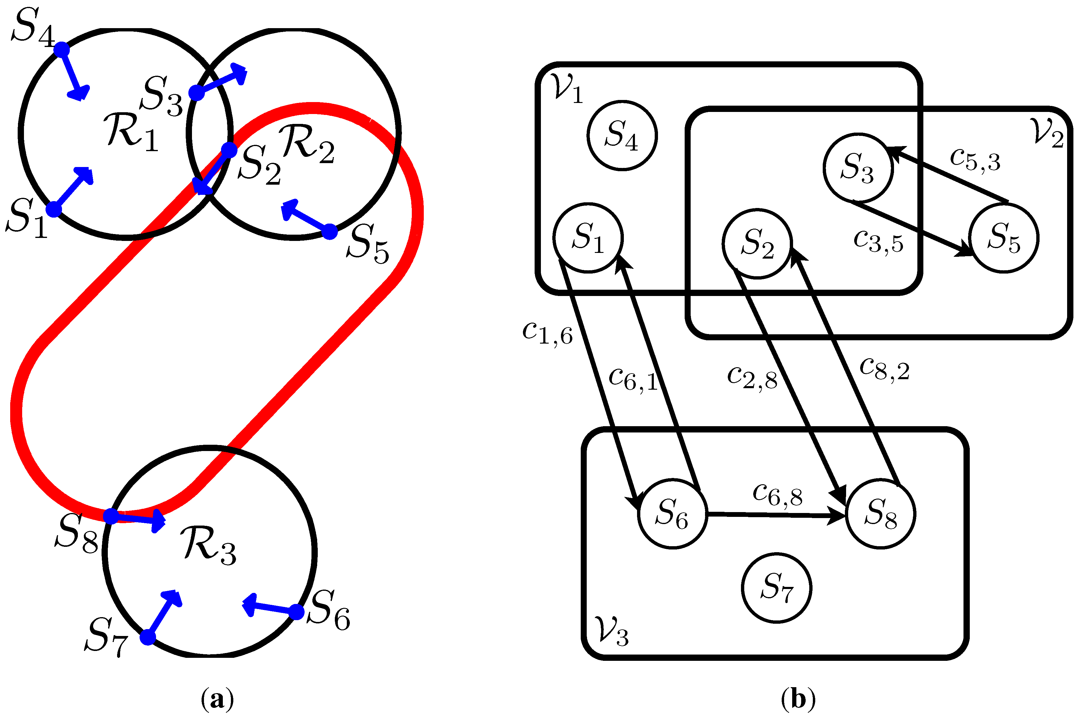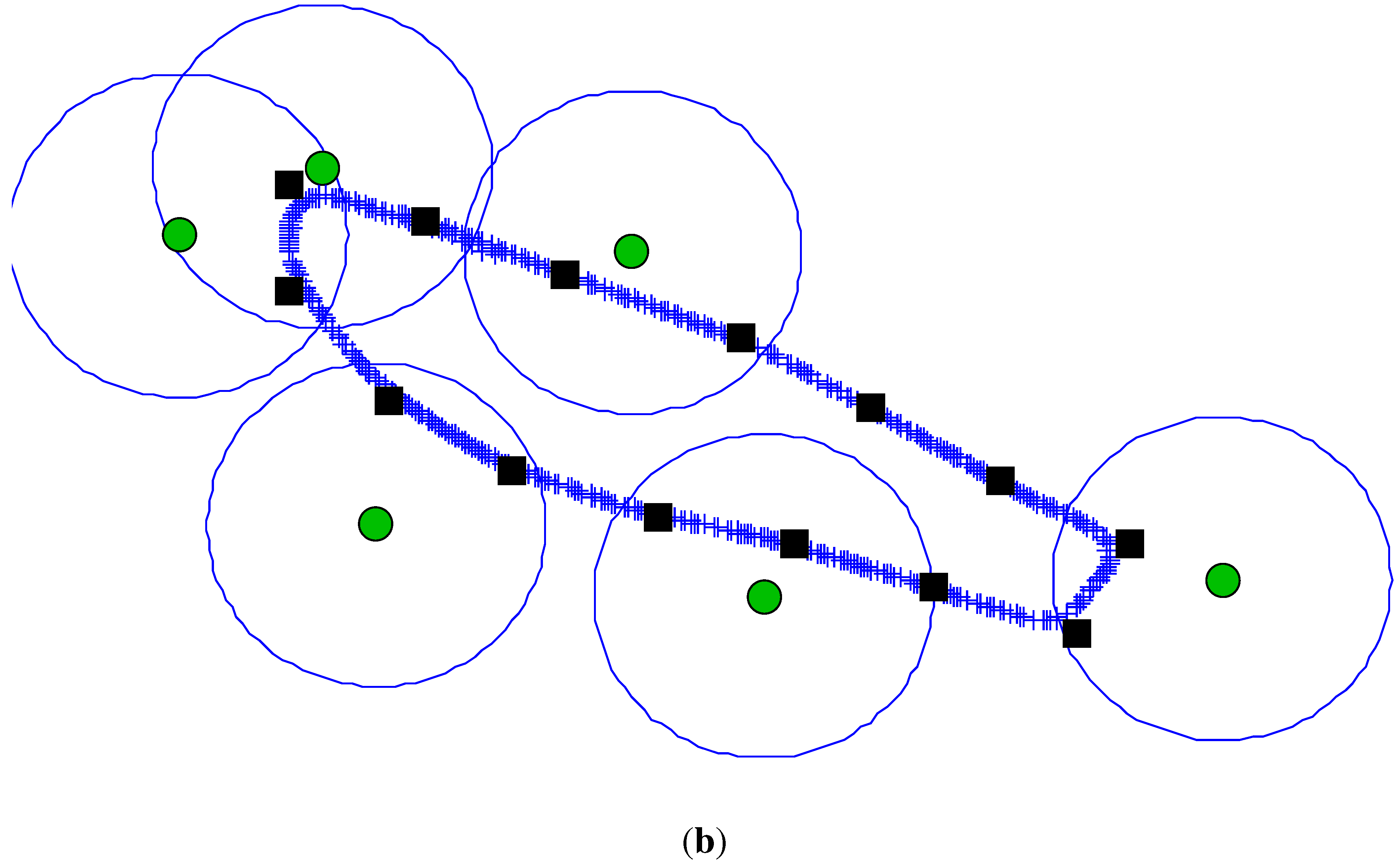The objective of the GTSP is to find a minimum cost cycle passing through each node set exactly one time. An example instance of Problem 2.2 can be seen in Figure 1(a).

Next, the GTSP can be converted to an Asymmetric TSP through a series of graph transformations due to Noon and Bean [17]. What follows is a brief summary of the Noon–Bean transformation from [17] as it is used in this work. The transformation is best described in three stages. The first stage converts the asymmetric GTSP to a GTSP with mutually exclusive node sets. The second stage converts the GTSP to the canonical form by eliminating intra-set arcs. Finally the third stage converts the canonical form to a clustered TSP and then to an Asymmetric TSP.

Figure 1. Example DTSPN with the corresponding “GTSP with intersecting node sets”. (a) Example instance of DTSPN with three circular regions ${\mathcal{R}}_1,{\mathcal{R}}_2,\text{and}{\mathcal{R}}_3$ and samples $S_1,S_2,\dots ,S_8$. The circuit through samples $S_2,\text{and},S_8$ is the optimal tour; (b) Problem (P0): A GTSP with intersecting node sets representation of the DTSPN example. Note: only an essential subset of arcs is shown for clarity of illustration.

Figure 1. Example DTSPN with the corresponding “GTSP with intersecting node sets”. (a) Example instance of DTSPN with three circular regions ${\mathcal{R}}_1,{\mathcal{R}}_2,\text{and}{\mathcal{R}}_3$ and samples $S_1,S_2,\dots ,S_8$. The circuit through samples $S_2,\text{and},S_8$ is the optimal tour; (b) Problem (P0): A GTSP with intersecting node sets representation of the DTSPN example. Note: only an essential subset of arcs is shown for clarity of illustration.

3.1. Stage 1

We begin by restating the problem above in a compact manor to facilitate the discussion. Problem $(P0)$ is a GTSP defined by the graph ${\mathcal{G}}^0:=({\mathcal{N}}^0,{\mathcal{A}}^0,{\mathcal{V}}^0)$ with the corresponding cost vector $c^0$. An example of Problem (P0) is shown in Figure 1(b). The first stage converts the GTSP $(P0)$ to a new problem $(P1)$ which is a GTSP with mutually exclusive node sets. This is done by first eliminating any arcs from ${\mathcal{A}}^0$ that do not enter at least one new node set.

Problem $(P1)$ is a GTSP defined by the graph ${\mathcal{G}}^1:=({\mathcal{N}}^1,{\mathcal{A}}^1,{\mathcal{V}}^1)$ with the corresponding cost vector $c^1$. Where ${\mathcal{N}}^1={\mathcal{N}}^0$, and ${\mathcal{V}}^1={\mathcal{V}}^0$. The arc set ${\mathcal{A}}^1$ is formed by first setting ${\mathcal{A}}^1={\mathcal{A}}^0$, and then removing any edges that do not enter at least one new node set. Let $\mathcal{M}(i)$ denote the set of node sets of which node i is a member, i.e., if $i\in {\mathcal{V}}_k$, then $k\in \mathcal{M}(i)$. 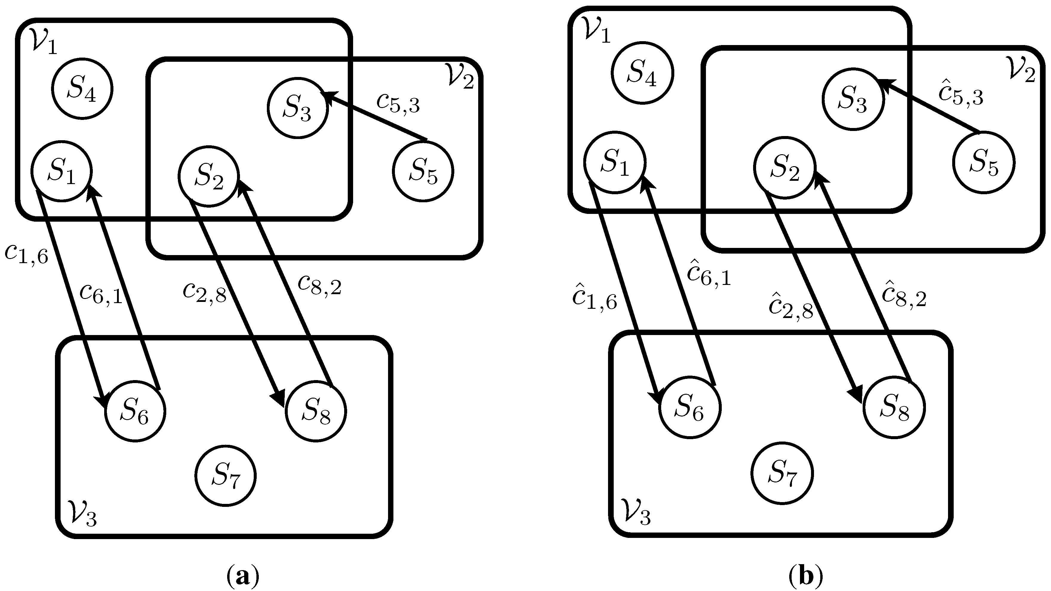For every $(i,j)\in {\mathcal{A}}^0$, if $\mathcal{M}(j)\subset \mathcal{M}(i)$, then remove the arc $(i,j)$ from set ${\mathcal{A}}^1$, see Figure 2(a).

Figure 2. Example of Problem (P1) and Problem (P2) from Stage 1 of transformation. (a) Problem (P1): Any arcs that do not enter at least one new node set $\{(3,5)$ and $(6,8)\}$ have been removed from the graph in Problem (P0); (b) Problem (P2): A large finite cost α is added to each edge. Here ${\widehat{c}}_{i,j}=c_{i,j}^2$, where $c_{i,j}^2$ is defined in Equation (4).

Figure 2. Example of Problem (P1) and Problem (P2) from Stage 1 of transformation. (a) Problem (P1): Any arcs that do not enter at least one new node set $\{(3,5)$ and $(6,8)\}$ have been removed from the graph in Problem (P0); (b) Problem (P2): A large finite cost α is added to each edge. Here ${\widehat{c}}_{i,j}=c_{i,j}^2$, where $c_{i,j}^2$ is defined in Equation (4).

Next, a constant is added to the cost of each arc entering a new node set. Problem $(P2)$ is a GTSP defined by the graph ${\mathcal{G}}^2:=({\mathcal{N}}^2,{\mathcal{A}}^2,{\mathcal{V}}^2)$ with the corresponding cost vector $c^2$. Where ${\mathcal{N}}^2={\mathcal{N}}^1$, ${\mathcal{A}}^2={\mathcal{A}}^1$, and ${\mathcal{V}}^1={\mathcal{V}}^0$. Notice that all arc costs are nonnegative. We now define a finite, positive constant α as,

$$\begin{array}{c}\hfill \infty >\alpha \ge \sum _{(i,j)\in {\mathcal{A}}^1}{c}_{i,j}^1\end{array}$$

(3)

For every arc $(i,j)\in {\mathcal{A}}^1$, set the cost of the arc $(i,j)\in {\mathcal{A}}^2$ in the following manner,

$$\begin{array}{c}\hfill c_{i,j}^2=(|\mathcal{M}(j)-\{\mathcal{M}(i)\cap \mathcal{M}(j)\}|)\alpha +c_{i,j}^1\end{array}$$

(4)

Here $\left|Z\right|$, represents the cardinality of the set Z. Notice that Equation (4) adds to the original arc cost an additional cost of α for each new node set entered by arc $(i,j)$. An example of Problem (P2) can be seen in Figure 2(b), where ${\widehat{c}}_{i,j}$ represents $c_{i,j}^2$.

Next, any nodes that belong to more than one node set are duplicated and placed in different node sets so as to allow each node to have membership in only one node set. Problem $(P3)$ is a GTSP over the graph ${\mathcal{G}}^3:=({\mathcal{N}}^3,{\mathcal{A}}^3,{\mathcal{V}}^3)$ with the corresponding cost vector $c^3$. The set of nodes ${\mathcal{N}}^3$ will be populated with the same set of nodes in ${\mathcal{N}}^2$ plus the additional nodes created to account for the nodes that fall into multiple node sets. For every $i\in {\mathcal{N}}^2$, create $|\mathcal{M}(i)|$ nodes and assign each to a different node set. For all $k\in \mathcal{M}(i)$, add the node $i_k$ to ${\mathcal{N}}^3$, and to the node set ${\mathcal{V}}_k^3$. This insures that $|\mathcal{M}(i_k)|=1$. Any arcs to and from the original nodes are duplicated as well. For every arc $(i,j)\in {\mathcal{A}}^2$, create the arc $(i^p,j^q)\in {\mathcal{A}}^3$ with the corresponding cost $c_{i^p,j^q}^3=c_{i,j}^2$ for every $p\in \mathcal{M}(i)$ and $q\in \mathcal{M}(j)$. In addition, zero cost arcs are added between all the spawned nodes of each multiple membership node. For each node $i\in {\mathcal{N}}^2$ with multiple node set membership $|\mathcal{M}(i)|>1$, create arcs $(i^p,i^q)\in {\mathcal{A}}^3$ with associated costs $c_{i^p,i^q}^3=0$ for all $p\in \mathcal{M}(i),q\in \mathcal{M}(i)$, such that $p\ne q$. 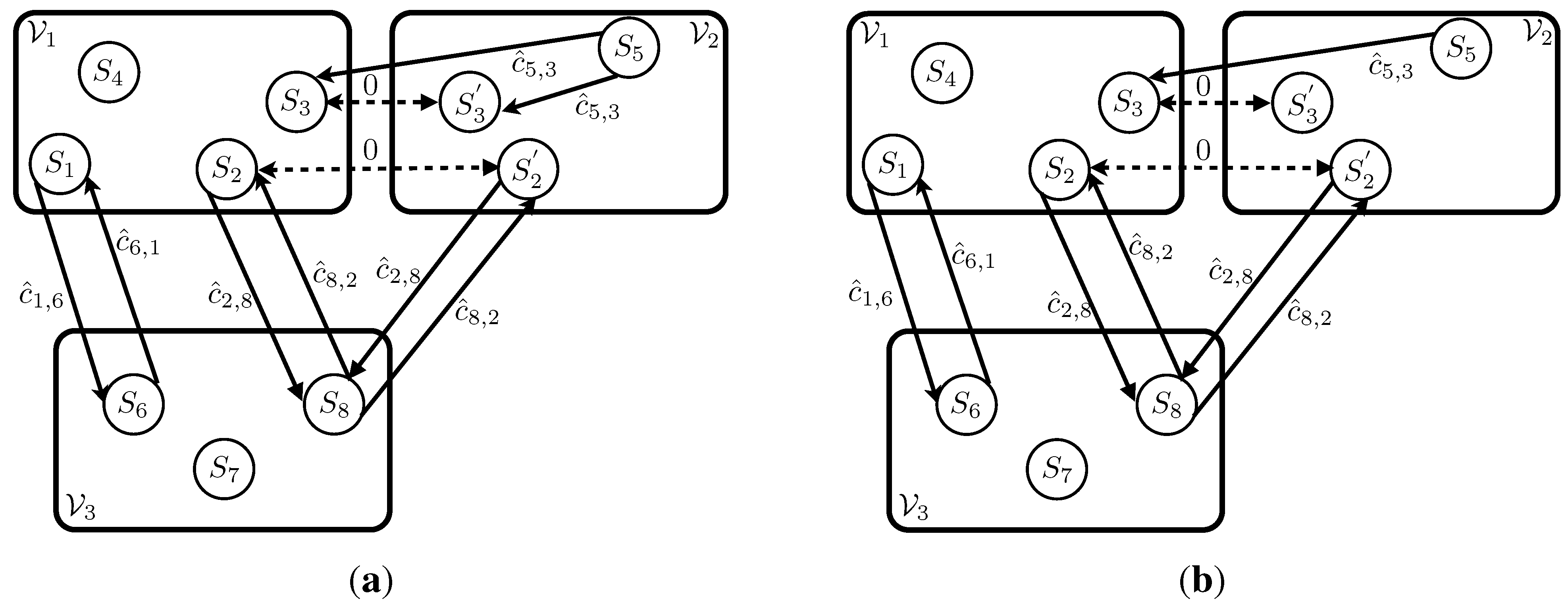See Figure 3(a) for an example of Problem (P3).

Figure 3. Example of Problem (P3) and Problem (P4) from Stage 1 and Stage 2 of transformation. (a) Problem (P3): Nodes $S_2$ and $S_3$ from (P2) lie in multiple node sets. These nodes are duplicated and the spawned nodes $S_{2^{\prime }}$ and $S_{3^{\prime }}$ are placed in node set ${\mathcal{V}}_2$. Zero cost arcs (dashed arrows) are added connecting $S_2$ to $S_{2^{\prime }}$ and $S_3$ to $S_{3^{\prime }}$; (b) Problem (P4): The intra-set arc $(5,3^{{}^{\prime }})$ from Problem (P3) is removed.

Figure 3. Example of Problem (P3) and Problem (P4) from Stage 1 and Stage 2 of transformation. (a) Problem (P3): Nodes $S_2$ and $S_3$ from (P2) lie in multiple node sets. These nodes are duplicated and the spawned nodes $S_{2^{\prime }}$ and $S_{3^{\prime }}$ are placed in node set ${\mathcal{V}}_2$. Zero cost arcs (dashed arrows) are added connecting $S_2$ to $S_{2^{\prime }}$ and $S_3$ to $S_{3^{\prime }}$; (b) Problem (P4): The intra-set arc $(5,3^{{}^{\prime }})$ from Problem (P3) is removed.

To summarize, Stage 1 of the Noon–Bean transformation takes GTSP with intersecting node sets and transforms it into a GTSP with mutually exclusive node sets. The following theorem from [17] summarizes the relationships between problems $(P0)$, $(P1)$, $(P2)$, and $(P3)$.

Theorem 3.1 (Noon and Bean [17]). Given a GTSP in the form of $(P0)$, we can transform the problem to a problem of the form of $(P3)$. Given an optimal solution to $(P3)$ with cost less than $(m+1)\alpha$, we can construct an optimal solution to $(P0)$. If an optimal solution to $(P3)$ has a cost greater than or equal to $(m+1)\alpha$, the problem $(P0)$ is infeasible.

3.2. Stage 2

The second stage takes the GTSP with mutually exclusive node sets and eliminates any intra-set arcs, leaving a GTSP in “canonical form.” Define a problem $(P4)$ that differs from problem $(P3)$ only by the arcs and arc costs. Problem $(P4)$ is a GTSP over the graph ${\mathcal{G}}^4:=({\mathcal{N}}^4,{\mathcal{A}}^4,{\mathcal{V}}^4)$ with the corresponding cost vector $c^4$ where ${\mathcal{N}}^4={\mathcal{N}}^3$ and ${\mathcal{V}}^4={\mathcal{V}}^3$. The arc set ${\mathcal{A}}^4$ is populated in the following manner. For every $i,j$ pair of nodes in ${\mathcal{N}}^3$ for which $\mathcal{M}(i)\ne \mathcal{M}(j)$, calculate the lowest cost path from i to j over the arc set ${\mathcal{A}}_{i,j}\subseteq {\mathcal{A}}^3$. An arc $(k,l)\in {\mathcal{A}}_{i,j}$ if the following four conditions hold,

• $\mathcal{M}(k)\subseteq \mathcal{M}(i)\cup \mathcal{M}(j)$,
• $\mathcal{M}(l)\subseteq \mathcal{M}(i)\cup \mathcal{M}(j)$,
• if $\mathcal{M}(l)=\mathcal{M}(i)$ then $\mathcal{M}(k)$ must also equal $\mathcal{M}(i)$,
• if $\mathcal{M}(k)=\mathcal{M}(j)$ then $\mathcal{M}(l)$ must also equal $\mathcal{M}(j)$.

If the shortest path has finite cost, add the arc $(i,j)$ to the arc set ${\mathcal{A}}^4$, and set the corresponding arc cost $c_{i,j}^4$ equal to the shortest path cost. If no feasible path exists, then the arc $(i,j)$ will not be part of ${\mathcal{A}}^4$. The problem defined on ${\mathcal{G}}^4$ is now in the GTSP canonical form with mutually exclusive node sets and no intra-set arcs. See Figure 3(b) for an example of Problem (P4). The following theorem from [17] establishes the correctness of the transformation in Stage 2.

Theorem 3.2 (Noon and Bean [17]). Given an optimal solution, $y^{*}$, to $(P4)$, we can construct the optimal solution, $x^{*}$, to $(P3)$.

3.3. Stage 3

The third stage of the transformation converts the canonical GTSP to a “clustered” TSP. Problem $(P5)$ is a clustered TSP over the graph ${\mathcal{G}}^5:=({\mathcal{N}}^5,{\mathcal{A}}^5)$ with the corresponding cost vector $c^5$ where ${\mathcal{N}}^5={\mathcal{N}}^4$. For every node set ${\mathcal{V}}_i$ corresponding to nodes in ${\mathcal{N}}^4$, define a cluster ${\mathcal{C}}_i$ corresponding to the nodes in ${\mathcal{N}}^5$. The nodes in each cluster are first enumerated. Let $i^1,i^2,\dots ,i^r$ denote the ordered nodes of ${\mathcal{C}}_i$ where r represents the cardinality of the cluster, $r=|{\mathcal{C}}_i|$. Next, a zero cost cycle is created for each cluster by adding zero cost edges between consecutive nodes in each cluster and connecting the first node to the last. For each cluster i with $r>1$, add the arcs $(i^1,i^2),(i^2,i^3),\dots ,(i^{r-1},i^r),(i^r,i^1)$ to ${\mathcal{A}}^5$, and for each of these intra-cluster arcs assign a zero cost, i.e., $c_{i^1,i^2}^5=\cdots =c_{i^r,i^1}^5=0$. The inter-set edges are then shifted so they emanate from the previous node in its cycle. For every inter-set arc $(i^k,j^l)\in {\mathcal{A}}^4$, with $k>0$, create the arc $(i^{k-1},j^l)\in {\mathcal{A}}^5$ with the corresponding cost, $c_{i^{k-1},j^l}^5=c_{i^k,j^l}^4$. For each interest arc $(i^1,j^l)\in {\mathcal{A}}^4$, create the arc $(i^r,j^l)\in {\mathcal{A}}^5$ with the corresponding cost, $c_{i^r,j^l}^5=c_{i^1,j^l}^4$, where $r=|{\mathcal{C}}_i|$. 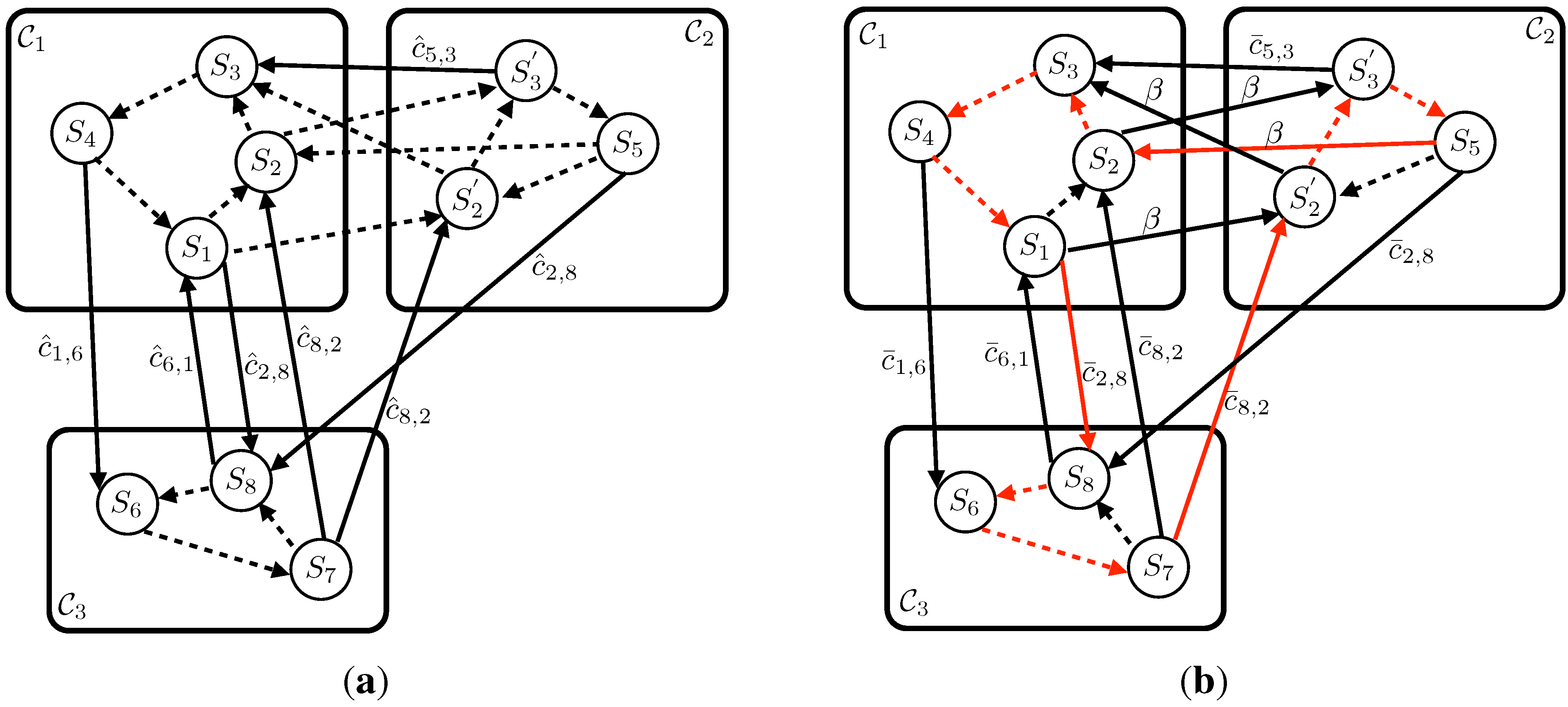See Figure 4(a) for an example of Problem (P5).

Finally, the clustered TSP is converted to an ATSP by adding a large finite cost to each inter-cluster arc cost.

Problem $(P6)$ is a ATSP over the graph ${\mathcal{G}}^6:=({\mathcal{N}}^6,{\mathcal{A}}^6)$ with the corresponding cost vector $c^6$ where ${\mathcal{N}}^6={\mathcal{N}}^5$ and ${\mathcal{A}}^6={\mathcal{A}}^5$. The arc costs are differ from $(P5)$ in the following way. For every arc $(i,j)\in {\mathcal{A}}^6$, if i and j belong to the same clusters in $(P5)$, then $c_{i,j}^6=c_{i,j}^5$. If i and j belong to different clusters in $(P5)$, then

$$\begin{array}{c}\hfill c_{i,j}^6=c_{i,j}^5+\beta \end{array}$$

(5)

where

$$\begin{array}{c}\hfill \infty >\beta >\sum _{(i,j)\in {\mathcal{A}}^5}{c}_{i,j}^5\end{array}$$

(6)

An example can be seen in Figure 4(b), where ${\overline{c}}_{i,j}$ depicts $c_{i,j}^6$. The optimal tour is shown in red.

The following theorem from [17] establishes the correctness of the transformation in Stage 3.

Theorem 3.3 (Noon and Bean [17]). Given a canonical GTSP in the form of $(P4)$ with n node sets, we can transform the problem into a standard TSP in the form of $(P6)$. Given an optimal solution $y^{*}$ to $(P6)$ with $c^6{y}^{*}<(n+1)\beta$, we can construct an optimal solution $x^{*}$ to $(P4)$.

Figure 4. Example of Problem (P5) and Problem (P6) from Stage 3 of transformation. (a) Problem (P5): The clustered TSP is created by forming zero cost intra-set cycles and adjusting the originating node in each inter-set arc; (b) Problem (P6): A large finite cost β is added to each inter-set edge. Here ${\overline{c}}_{i,j}=c_{i,j}^6$, where $c_{i,j}^6$ is defined in Equation (5). The optimal tour is shown in red with a cost of ${\widehat{c}}_{8,2}+\beta +{\widehat{c}}_{2,8}$.

Figure 4. Example of Problem (P5) and Problem (P6) from Stage 3 of transformation. (a) Problem (P5): The clustered TSP is created by forming zero cost intra-set cycles and adjusting the originating node in each inter-set arc; (b) Problem (P6): A large finite cost β is added to each inter-set edge. Here ${\overline{c}}_{i,j}=c_{i,j}^6$, where $c_{i,j}^6$ is defined in Equation (5). The optimal tour is shown in red with a cost of ${\widehat{c}}_{8,2}+\beta +{\widehat{c}}_{2,8}$.

3.4. Performance Comparison

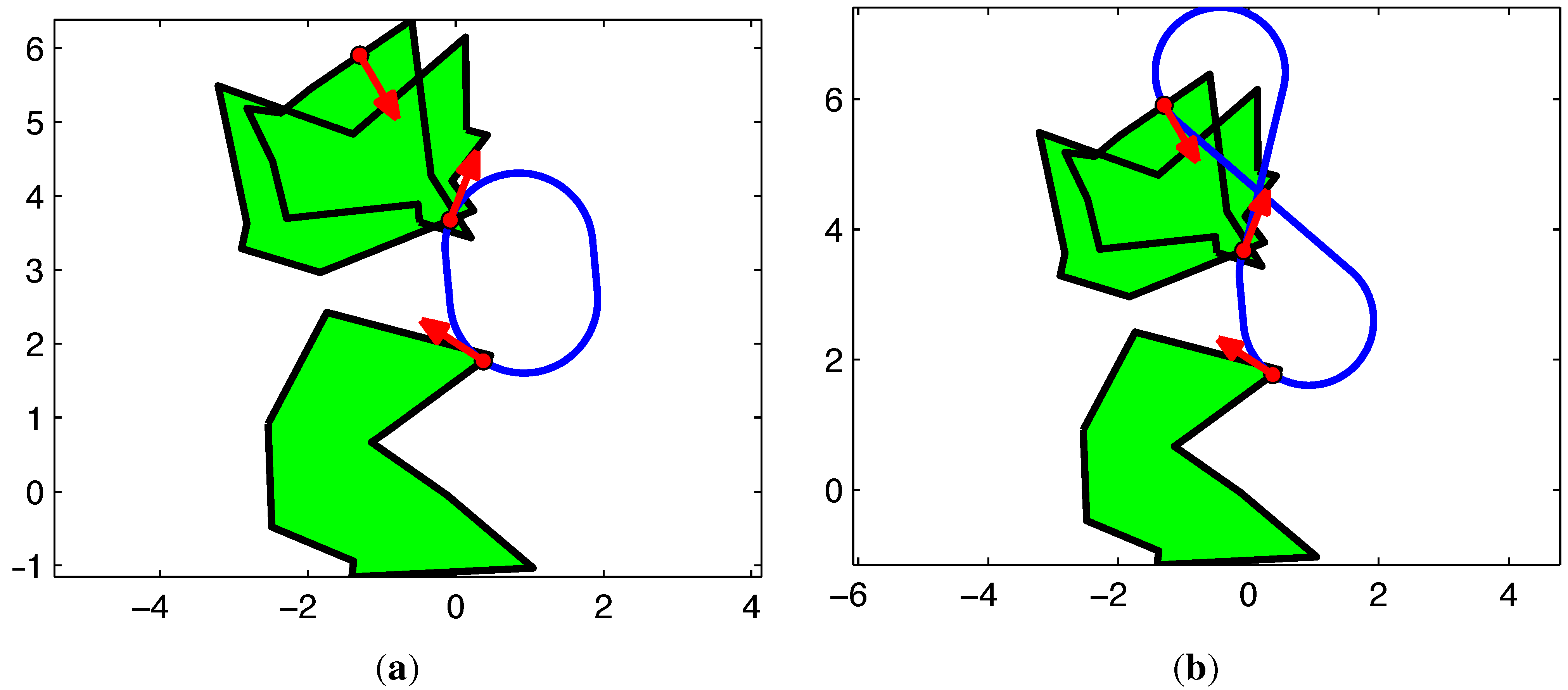
The Intersecting Regions Algorithm (IRA) proposed here is similar to the Resolution Complete Method (RCM) proposed in [15] with the key exception that we use the fact that visiting one of the samples in the intersection of multiple regions achieves the goal of visiting all the regions in the intersection. Figure 5 illustrate this key difference. The RCM requires mutually exclusive node sets for the conversion from DTSPN to a GTSP with disjoint node sets. To meet this requirement, samples are assigned directly to the node set of the region from whose boundary they are drawn, as depicted in Figure 5(b). If multiple regions overlap and a sample lies in the intersection, IRA assigns this sample to all the node sets corresponding to the intersecting regions, as depicted in Figure 5(a), while RCM does not. The IRA then uses this additional information in the optimization.

Theorem 3.4 (IRA Performance). Given $\rho >0$, the set of $n\ge 2$ possibly intersecting regions, R, and the set of m sample configurations, S, let $T_{IRA}$ and $T_{RCM}$ denote the tours produced by IRA and the RCM [15], respectively. Then the length of $T_{IRA}$ is no greater than that of $T_{RCM}$,

$$\begin{array}{c}\hfill \mathrm{length}(T_{IRA})\le \mathrm{length}(T_{RCM})\end{array}$$

(7)

Proof. [Proof of Theorem 3.4] Let $T=\{S_1,S_2,\dots ,S_n\}$ be a feasible tour, and note that both IRA and RCM minimize the tour length plus an additive constant while ensuring that all regions are visited. The difference is that IRA may produce tours visiting fewer than n unique samples, should some samples lie in the multiple regions. In particular, the IRA ensures that each leg of the tour enters at least one new region, by construction. Therefore, in performing the optimization IRA will either consider T, or subset of T, in which samples at the end of legs not entering an unvisited region have been removed. Due to the Dubins distance function satisfying the triangle inequality [20], a tour that visits a redundant sample will be longer than a tour that visits a subset of the samples. The optimal tour $T_{IRA}$ cannot be longer than $T_{RCM}$, because both optimize over the same set of feasible tours except for the tours in which IRA bypasses these unneeded samples.     ☐

The property resolution complete method as used in [15], dictates that the method converges to a solution at least as good as any nonisolated optimum solution as the number of sample configurations goes to infinity.

Corollary 3.5 (IRA is Resolution Complete). Given $\rho >0$, the set of $n\ge 2$ possibly intersecting regions, R, and the set of m sample configurations, S drawn from a Halton quasi-random sequence [21] as in RCM, then IRA is Resolution Complete.

Proof. [Proof of Corollary 3.5] From [15], the RCM is a resolution complete method and converges as the number of samples goes to infinity, and from Theorem 3.4, we have shown that for the same set of sample configurations IRA will produce a tour that is no longer than RCM.     ☐

Figure 5. A comparison of IRA and RCM on an example DTSPN instance with three regions and three sample poses. (a) Example Tour: IRA, Tour Length $=7.7$; (b) Example Tour: RCM, Tour Length $=15.4$.

Figure 5. A comparison of IRA and RCM on an example DTSPN instance with three regions and three sample poses. (a) Example Tour: IRA, Tour Length $=7.7$; (b) Example Tour: RCM, Tour Length $=15.4$.

3.5. Complexity of Intersecting Regions Algorithm

We have provided an algorithm that takes advantage of sample configurations that lie in overlapping regions, and we have shown that this algorithm produces a tour that is no longer than the previous best algorithms in the literature. However, the size of the ATSP is increased by the number of multiple node set duplicate nodes. Given m samples from n regions, this algorithm will compute the ATSP over at most $mn$ nodes. The worst case computational complexity of the Noon and Bean transformation [17] is $O(m^2{n}^4)$. Then the worst case complexity for solving the ATSP using the modified version of Christofides’ algorithm provided in [22] is $O(m^3{n}^3)$.

4. Numerical Results

In Theorem 3.4 we have shown that for the same sample set, IRA will perform no worse than the resolution complete method from [15], but at the cost of solving a larger ATSP problem when there exist samples that are contained in multiple regions. In this section, we use Monte Carlo simulation to investigate the level of performance improvement that can be gained as well as the degree of increase in the size of the resulting ATSP by using IRA compared with the RCM.

Figure 6. Simulation results for 100 Monte Carlo trials where both IRA and RCM optimized over the same 50 sample poses. (a) The color represents the average of the ratio of the tour length under IRA to the tour length under the RCM planning algorithm. Here the red regions indicate near parity in performance while the blue regions indicate that IRA produced tours that are approximately half the length of tours produced by the RCM algorithm; (b) The color represents the average of the ratio of the size of the ATSP solved under IRA to the size of the ATSP solved under the RCM planning algorithm. Here the blue regions indicate near parity in size while the red regions indicate that IRA increased the size of the ATSP by as much as four times.

Figure 6. Simulation results for 100 Monte Carlo trials where both IRA and RCM optimized over the same 50 sample poses. (a) The color represents the average of the ratio of the tour length under IRA to the tour length under the RCM planning algorithm. Here the red regions indicate near parity in performance while the blue regions indicate that IRA produced tours that are approximately half the length of tours produced by the RCM algorithm; (b) The color represents the average of the ratio of the size of the ATSP solved under IRA to the size of the ATSP solved under the RCM planning algorithm. Here the blue regions indicate near parity in size while the red regions indicate that IRA increased the size of the ATSP by as much as four times.

The centers of circular regions of variable but homogeneous diameters are randomly placed in a square of variable side length. By varying both the size of regions and the area in which the centers of the regions are confined we are able to vary the degree of overlap. The turning radius of the UAV ρ is set to unit radius. To solve for the tours we used the symmetric TSP solver linkern available at [23], which uses the Chained Lin–Kernighan Heuristic from [24]. The radii of the circular regions were varied over $\{0.5,0.75,1.00,\dots ,5.5\}$, and the length of the sides of the square were varied over $\{5,5.5,\dots ,15\}$.

For the first test, we ran 100 trials where 10 regions were randomly placed in the bounding box and 50 samples were drawn from the boundaries of the regions. The results can be seen in Figure 6, where the average ratio of the length of the tours found by the IRA to those found by RCM are displayed for each test configuration (Figure 6(a)) as well as the average ratio of the size of the resulting ATSP (Figure 6(b)). In a second test, we repeated the same test parameters where IRA optimized over 50 sample poses, but allowed the RCM to optimize over the same 50 samples plus an additional sample for each duplicated node in the IRA. These extra samples ensured that both algorithms solved the same size ATSP. The results can be seen in Figure 7, where the average ratio of the length of the tours found by the IRA to those found by RCM are displayed for each test configuration. In both instances, it is clear that for small regions and large bounding box (bottom right of plots), there is little to no overlap, and the two algorithms perform equivalently. The tests of interest are when the regions grow, and the bounding area shrinks (moving from bottom right to top left). For these cases we see that on average, IRA finds tours that are nearly half the length of RCM. It should be noted that as the density increases, there becomes a point where a single sample will be contained in all regions (the top left corner). In this case, RCM would still visit n samples (one from each region) while IRA would only visit the single sample contained in all regions. In practice there is no need for planning once it is recognized that a single loiter circle will visit all the regions, thus both algorithms were assigned the length of one loiter radius. It should also be noted that the size of the resulting ATSP is increased by only as much as $4\times$, which is significantly less than the worst case analysis would predict $(10\times )$.

Figure 7. Simulation results for the where IRA optimized over 50 sample poses and RCM optimized over the same 50 samples plus an additional sample for each duplicated node in the IRA. These extra samples ensured that both algorithms solved the same size ATSP.

Figure 7. Simulation results for the where IRA optimized over 50 sample poses and RCM optimized over the same 50 samples plus an additional sample for each duplicated node in the IRA. These extra samples ensured that both algorithms solved the same size ATSP.

5. Demonstration

The algorithm presented here was demonstrated as part of a large field test conducted in June 2011 at Camp Roberts, CA by a team consisting of Teledyne Scientific Company, the University of California, Santa Barbara, the U.S. Army Research Laboratory, the U.S. Army Engineer Research and Development Center, and IBM UK. The goal of the field test included the integration of multiple autonomously controlled UAVs to gather information regarding the detection and localization of multiple acoustic events by sparsely deployed ground sensors, and the use of the International Technology Alliance (ITA) Sensor Network Fabric [25].

A schematic of the system used in the deployment is shown in Figure 8(a). We deployed six ToA sensors over a region that was roughly $1.3$ km $\times 0.5$ km in size. We used GPS receivers at each sensor to estimate their locations and synchronize them in time. Two propane cannons that have acoustic characteristics similar to artillery were fired randomly and potentially close to one another in time. A UAV traveled along a DTSPN tour produced by IRA, gathering ToAs and inferring possible event locations. When the inference algorithm had sufficient confidence in a candidate event, it dispatched a second UAV, fitted with a gimbaled camera, to fly over the estimated location and image the source. The data gathering and event imaging was done continuously, with the events being imaged on a first come first served basis.

Figure 8. The configuration of sensors and UAV trajectory during the field demonstration at Camp Roberts, CA. (a) Field Demonstration Description. The acoustic sensors visited by the data collecting UAV are shown as yellow dots; (b) The blue lines represent the GPS logs of the path taken by data collecting UAV during the test. The desired path was sent to the autopilot via the square waypoints. The sensors and communication regions are represented by green and blue circles respectively.

Figure 8. The configuration of sensors and UAV trajectory during the field demonstration at Camp Roberts, CA. (a) Field Demonstration Description. The acoustic sensors visited by the data collecting UAV are shown as yellow dots; (b) The blue lines represent the GPS logs of the path taken by data collecting UAV during the test. The desired path was sent to the autopilot via the square waypoints. The sensors and communication regions are represented by green and blue circles respectively.

5.1. Modifications for the Demonstration

The Intersecting Regions Algorithm from above is designed as a path planning algorithm. If the planned path is followed in an open-loop fashion, the system is susceptible to disturbances such as wind and modeling errors. As such the IRS was modified slightly to be more robust to disturbances such as wind as well as allow for waypoint control of the UAV. The first modification of the routing algorithm reduced the size of the communication regions in the optimization to ensure that the resulting path would penetrate the original communication region even under the influence of small disturbances. The second modification involved sampling the desired path to obtain a finite sequence of waypoints to command to the UAV autopilot.

The route flown by the mule-UAV and the communication regions used in the DTSPN path planning algorithm are shown in Figure 8(b). It took on average two minutes and fifty seconds for the mule-UAV to complete the circuit and collect measurements from all ground sensors. This time is conservative due to the modifications to the algorithm that ensure that the UAV enters into each communication region (radius $=200$ m).

6. Conclusions

We have introduced an algorithm addressing the Dubins Traveling Salesman Problem with Neighborhoods. This algorithm samples the regions and then utilizes the Noon and Bean transformation [17] for intersecting node sets to transform the problem to an ATSP. We show that for the same set of samples this method will produce a tour that is no longer than that of [15] and presented numerical results that show performance improvement when there is overlap in the regions of interest.

There are many directions in which this work may be extended. Although we have focused on the Dubins model for a fixed wing UAV, the IRA could be applied to any nonholonomic vehicle whose node to node cost is well defined. Also, it is of interest to understand if a deterministic way to sample the configurations would be of benefit in possibly reducing the number samples needed to achieve a certain level of performance. For instance, if there is significant overlap, would it be beneficial to ensure that at least one sample is taken from each subregion. Finally, for large instances of the DTSPN, we are interested in comparing the performance of this method with direct GTSP solvers such as the memetic algorithm due to Gutin and Karapetyan [18].