Linear Time Local Approximation Algorithm for Maximum Stable Marriage

Abstract

We consider a two-sided market under incomplete preference lists with ties, where the goal is to find a maximum size stable matching. The problem is APX-hard, and a $3/2$-approximation was given by McDermid [1]. This algorithm has a non-linear running time, and, more importantly needs global knowledge of all preference lists. We present a very natural, economically reasonable, local, linear time algorithm with the same ratio, using some ideas of Paluch [2]. In this algorithm every person make decisions using only their own list, and some information asked from members of these lists (as in the case of the famous algorithm of Gale and Shapley). Some consequences to the Hospitals/Residents problem are also discussed.

1. Introduction

In 1962, Gale and Shapley [3] gave their famous simple deferred acceptance algorithm, which always finds stable matching in a two-sided market. If incomplete lists and ties are allowed in the preference lists, their algorithm still works, and gives some stable matching. However, in this case, we are usually interested in not only finding some stable matching, but one with maximum size. This problem (usually called MAX-SMTI) is APX-hard, and probably cannot be approximated within a factor of $4/3$. McDermid [1] gave the first $3/2$-approximation using our previous $3/2$-approximation for the case, when ties are only on one side of the market [4].

In this paper, we give a much simpler algorithm than the one he gave, which is only a slight modification of the historical algorithm of Gale and Shapley. It also gives $3/2$-approximation, but in linear time. The proof of the approximation ratio is uncomplicated, thus it serves as a good example for teaching purposes.

We call a mechanism natural if participants need not make any difficult computation and are not required to make illogical decisions. For several practice motivated models in Economics, natural mechanisms are more efficient than “artificial" ones.

In this paper, we make difference between global and local algorithms. When we speak about a global algorithm, we assume that there is a centralized decision mechanism, having all possible information (here: the preference lists of all participants). A global algorithm is called linear time if the number of steps it takes is some constant times the size of the input (usually the total length of the preference lists).

A local algorithm is quite restricted compared to a global algorithm. Here, every participant must have his/her own decision mechanism without having any global information. Besides his/her own information, a participant can only ask data from his/her acceptable partners. In real life, we have many circumstances when this is true for the participants. Therefore, designing a local information mechanism is an important goal. In this model, we assume everyone has his/her own list sorted at the beginning, and a local algorithm is called linear time if the number of steps any participant needs is some constant times the size of the input (length of the preference list) of that particular participant.

We will give both linear time global and linear time local algorithms for approximating the maximum size stable marriage problem, moreover in our local algorithm every participant of the two-sided market will make only very natural and rational decisions.

An instance of the stable marriage problem consists of a set U of men, a set W of women, and a preference list for each person; that is, a weak linear order (ties are allowed) of some participants (thus, in this paper, we are dealing with only the practical situation of incomplete lists) of the opposite gender. If $m\in U$ and $w\in W$, then a pair $mw$ is called acceptable if m is on the list of w and w is on the list of m. We model acceptable pairs with a bipartite graph $G=(U,W,E)$, (where E is the set of acceptable pairs; we may assume that if w is not on the list of m then m is also missing from the list of w). Note, that total length of the lists is proportional to $\left|E\right|$. A matching in this graph consists of mutually disjoint acceptable pairs.

We store the weak order of the lists as priorities. For an acceptable pair $mw$, let $\mathrm{pri}(w,m)$ be an integer from 1 up to $\left|U\right|$ representing the priority of m for w. We say that $w\in W$ strictly prefers $m_1\in U$ to $m_2\in U$ if both $m_1$ and $m_2$ are acceptable for w, and $\mathrm{pri}(w,m_1)>\mathrm{pri}(w,m_2)$. Ties are represented by equal priorities, e.g., if $m_1$ and $m_2$ are tied in w’s list, then $\mathrm{pri}(w,m_1)=\mathrm{pri}(w,m_2)$. We will later break up some ties, dividing the men in a tie into two groups, and we will say, that w prefers one group to the other. So there will be a case that w prefers $m_1$ to $m_2$, but she does not strictly prefer $m_1$ to $m_2$, and in this situation we mean that $\mathrm{pri}(w,m_1)=\mathrm{pri}(w,m_2)$, but $m_1$ is in the preferred group and $m_2$ is not. If both of them are in the same group then we say $m_1$ and $m_2$ are alike for w.

We define $\mathrm{pri}(m,w)$ similarly. Of course, $\mathrm{pri}(m,w)$ is not related to $\mathrm{pri}(w,m)$. We represent these priorities in the figures by writing $\mathrm{pri}(m,w)$ and $\mathrm{pri}(w,m)$ close to the corresponding endvertex of edge $mw$. For a man m we will modify his list in either of two ways. Sometimes we delete a woman from the list. Sometimes (at a given point, when his list is empty) we will restore the original list of m. We mean by “favorite woman” of m, the most preferred woman still on m’s list; if there are more alike women on the top of the list, we choose one of them arbitrarily.

Remark. The author apologizes that the text of this paper is not politically correct. Just like the one of Gale and Shapley [3], or the phrases used in many other papers on this topic. It would indeed be possible to change the terminology, but we find this approach pretty well-mannered. 

Let M be a matching. If m is matched in M, or in other words, if m is engaged then we denote m’s fiancée by $M\left(m\right)$. Similarly we use $M\left(w\right)$ for the fiancé of an engaged woman w.

Definition 1 

A pair $mw$ is blocking M, if $mw\in E\setminus M$ (they are an acceptable pair and they are not matched) and

• w is either not engaged or w strictly prefers m to her fiancé, and
• m is either not engaged or m strictly prefers w to his fiancée.

Definition 2 

A matching is called stable if there is no blocking pair.

While there may be objections to the connotations of these words, for simplicity we use the term “lad” to represent a man who still has some women on his list, whom he did not propose to so far, and we use the term “old bachelor” to represent a man who was rejected by all acceptable women and decides to become inactive forever. Moreover we use the term “maiden” to represent a woman who did not get any proposal so far. Later we need to use some other similar terms, defined there.

It is well-known that every instance of the stable marriage problem has a stable matching, and it can be found in linear time. The celebrated algorithm of Gale and Shapley [3] is the following. (We give a precise definition of the algorithms, however in a rather informal format. We think that none the less this style can be somewhat annoying for people studying algorithms regularly, for the other part of the readers it helps understanding the essence of these simple algorithms).

A man can be either a lad or an old bachelor. A lad can be either active or engaged. A woman can be either maiden or engaged. At the beginning every man is an active lad and every woman is a maiden.

Algorithm GS 

While there exists an active man m, he proposes to his favorite woman w. If w accepts his proposal, they become engaged. If w rejects him, m deletes w from his list.

When a woman w gets a new proposal from man m, she always accepts this proposal, if she is a maiden. She also accepts this proposal, if she prefers m to her current fiancé. Otherwise she rejects m.

If w accepted m, then she rejects her previous fiancé, if there was one (breaks off her engagement), and becomes engaged to m.

If a man m was engaged to a woman w, and later w rejects him, then m becomes active again, and deletes w from his list.

If the list of m becomes empty, he will turn into an old bachelor and will remain inactive forever.

After Algorithm GS finishes, the engaged pairs make up the output matching M (we may imagine that this time all the engaged pairs get married).

Theorem 1 

(Gale and Shapley [3]) Algorithm GS always ends in a stable matching M. This algorithm runs in $O\left(\right|E\left|\right)$ time.

An interesting problem, motivated by applications, is to find a stable matching of maximum size. As the applications of this problem are important (see e.g., in [5,6], where detailed lists of known and possible applications are given that motivate investigating refined approximations), researchers started to develop good approximation algorithms in the past six years. We say that an algorithm is r-approximating, if it gives a stable matching M with size $\left|M\right|\ge (1/r)·|M_{\mathrm{opt}}|$, where $M_{\mathrm{opt}}$ is a stable matching of maximum size. Observe that after a run of GS no unmarried man and unmarried woman can form an acceptable pair. Consequently Algorithm GS gives a 2-approximation, and for complete bipartite graphs (every woman-man pair is acceptable), it gives the optimum. The first non-trivial approximation algorithm was given by Halldórsson et al. [7], where they gave a $13/7$-approximation if all ties are of length two. The breakthrough was achieved by Iwama, Miyazaki and Yamauchi [8], who gave a $15/8$-approximation (for any length of ties). This was later improved by Irving and Manlove [5] to a $5/3$-approximation for the special case, where ties are allowed on one side only, and moreover only at the ends of the lists. Their algorithm also applies to the Hospitals/Residents problem (see below) if residents have strictly ordered lists. If, moreover, ties are of size 2, Halldórsson et al. [7] gave an $8/5$-approximation and in [9] they described a randomized algorithm for this special case with expected ratio of $10/7$.

This problem is known to be NP-hard for even very restricted cases [10,11]. Moreover, it is APX-hard [12] and, supposing P ≠ NP, it cannot be approximated within a factor of strictly less than $21/19$, even if ties occur in the preference lists on one side only, furthermore, if every list is either totally ordered or consists of a single tied pair [7]. Moreover, refining the ideas of [7], Yanagisawa [13] proved that an approximation within a factor of $4/3-\epsilon$ implies $(2-{\epsilon }^{\prime })$-approximation of vertex cover, and this result also applies to the case when each tie has length two. If, moreover, ties occur only in the preference lists on one side only, it was proved in [7] that an approximation within a factor of $5/4-\epsilon$ has the same implication. We note that interestingly the minimization version (where we are looking for a stable matching of minimum size) is also APX-hard [12].

We proposed a simple linear time $5/3$-approximating algorithm (called GSA2) for the general case of this problem, first presented at the first MATCH-UP workshop (see in [4,14,15]), and at the same time, an even simpler $3/2$-approximation (called GSA1) was given for the special case where ties are allowed on one side only. For this algorithm, the proof was also very short, see Section 2. This is also valid for the practically important "Hospitals/Residents" problem, where the lists of the residents are strict, see Section 5.

During the talks given at the first MATCH-UP workshop in Reykjavík and at ESA in Karlsruhe, we posed several questions, conjectures and open problems. Many of them were answered in the meanwhile.

The conjecture stating that the performance ratio proved for GSA2 is sharp proved to be true by Yanagisawa [16], who gave a simple example where GSA2 really gives a matching of size exactly $\frac{3}{5}·\left|M_{\mathrm{opt}}\right|$.

Irving and Manlove [17] implemented a basic version of our algorithm for the one-sided-ties Hospitals/Residents problem and gave a detailed comparison with their best heuristic (which is not a local algorithm, and it needs some max-flow computation on an auxiliary graph). They tested the algorithms carefully with real-life and artificial data. They concluded that for the most cases their best heuristic executed the best, but, on the average, our algorithm also gave a stable assignment of size at least $99.41\%$ of their best one. We do not know of too many other examples, where an algorithm with a guaranteed approximation ratio is so close in practice to the best known heuristic.

For the one-sided-ties case, Iwama, Miyazaki, and Yanagisawa [18] gave a $25/17\approx 1.47$-approximation. They solved the relaxed version of an appropriate ILP formulation, and used the fractional optimum to guide the tie-breaking process. Besides this, their algorithm is similar to GSA1, but the analysis is much deeper. Of course, as they have to solve an LP, it gives non-linear running time, and needs global information, so does not yield a local algorithm. However we consider this result important, because they broke the $3/2$-approximation factor barrier.

We had a conjecture given forth in Reykjavík [4], stating that a simple modification and repetition of GSA2 gives $3/2$-approximation for the general problem. It was (partially) answered by McDermid [1], who gave the first $3/2$-approximation for the general case. He used GSA1 (and not GSA2), but not with simple repetitions, at some points he stopped the main algorithm, constructed an auxiliary graph, and solved a maximum matching problem on it. In short, he used novel and rather complicated techniques, and so his algorithm needs $O\left(n\sqrt{n}\right|E\left|\right)$ running time (where $n=\left|U\right|+\left|W\right|$), and his algorithm also needs global information, so it cannot be converted to a local algorithm.

Recently, Paluch, [2] gave a new $3/2$-approximation algorithm for the general case, claiming a linear running time. Her algorithm was still quite complicated, used many concepts, and the analysis was also lengthy. It was not shown that her algorithm is local, but it can be converted to a linear time local algorithm with some more efforts, like what was done in Section 4. (Parallel to this work, she also made significant simplifications, and after releasing the technical report version [19] of our algorithm, she made some further changes and improvements, see the newest version of Paluch’s algorithm in [20].)

In Section 2 we reformulate Algorithm GSA1 of [4,14,15], then in Section 3 we give a simple linear time $3/2$-approximation, with a simple proof of correctness. We lean on two important ideas of Paluch. Our new algorithm is a slightly modified version of GSA1 given in the next section, thus it is also very reminiscent of the traditional Algorithm GS. In Section 4 we detail how our new algorithm can be implemented to run in linear time, both for the global and the local version. Finally, in Section 5 we reformulate this algorithm for the Hospitals/Residents problem.

2. Men Have Strictly Ordered Lists

In this section we suppose that the lists of men are strictly ordered. From now on a man can be a lad, a bachelor or an old bachelor, where we use the term "bachelor" for a man who was rejected by all acceptable women once, but in this setup he remains active and starts again to propose every woman on his recovered list. If there are two men, $m_1$ and $m_2$ with the same priority on a woman w’s list, and $m_1$ is a lad but $m_2$ is a bachelor, then w prefers bachelor $m_2$ to lad $m_1$. In the description of the algorithm, differences from Algorithm GS are set in boldface.

Algorithm GSA1 

While there exists an active man m, he proposes to his favorite woman w. If w accepts his proposal, they become engaged. If w rejects him, m deletes w from his list.

When a woman w gets a new proposal from man m, she always accepts this proposal, if she is a maiden. She also accepts this new proposal, if she prefers m to her current fiancé. Otherwise she rejects m.

If w accepted m, then she rejects her previous fiancé, if there was one (breaks off her engagement), and becomes engaged to m.

If m was engaged to a woman w and later w rejects him, then m becomes active again, and deletes w from his list.

If the list of m becomes empty for the first time, he turns into a bachelor, his original list is recovered, and he reactivates himself. If the list of m becomes empty for the second time, he will turn into an old bachelor and will remain inactive forever.

This simple algorithm runs in $O\left(\right|E\left|\right)$ time, as there are at most $2\left|E\right|$ proposals altogether (however see Section 4 for the details). It is easy to see that Algorithm GSA1 gives a stable matching M.

Theorem 2 (2008) 

If men have strictly ordered preference lists, M is the output of Algorithm GSA1 and $M_{\mathrm{opt}}$ is a maximum size stable matching then $|M_{\mathrm{opt}}|\le \frac{3}{2}·\left|M\right|.$

Proof. 

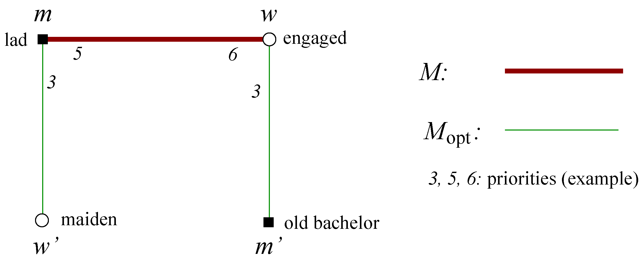
Take the union of M and $M_{\mathrm{opt}}$. We consider common edges as a two-cycle. Each component of $M\cup M_{\mathrm{opt}}$ is either an alternating cycle (of even length) or an alternating path. An alternating path component is called augmenting path if both end-edges are in $M_{\mathrm{opt}}$. An augmenting path is called short, if it consists of 3 edges (see Figure 1). It is enough to prove that in each component there are at most $3/2$ times as many $M_{\mathrm{opt}}$-edges as M-edges. This is clearly true for each component except for a short augmenting path.

Figure 1. A short augmenting path.

Figure 1. A short augmenting path.

We claim that a short augmenting path cannot exist. Suppose that $M\left(m\right)=w$, $M_{\mathrm{opt}}\left(m\right)=w^{\prime }\ne w$, $M_{\mathrm{opt}}\left(w\right)=m^{\prime }\ne m$ and that $m^{\prime }$ and $w^{\prime }$ are single in M. Observe first that $w^{\prime }$ is a maiden, thus she never got a proposal during Algorithm GSA1. Consequently m is a lad, who prefers w to $w^{\prime }$. As the algorithm finished, $m^{\prime }$ is an old bachelor, so he proposed to w also as a bachelor (see Figure 1), but w preferred m to $m^{\prime }$. Consequently w strictly prefers m to $m^{\prime }$. However, in this case edge $mw$ blocks $M_{\mathrm{opt}}$, a contradiction.                ☐

3. The New Algorithm for General Stable Marriage

For the new algorithm we use the following terms, most of which are familiar to the reader. A man can be either a lad, or a bachelor, or an old bachelor. A lad or a bachelor can be either active or engaged. If women $w_1$ and $w_2$ have the same priority on m’s list, and $w_1$ is maiden but $w_2$ is engaged, then m prefers maiden $w_1$ to engaged $w_2$. An engaged lad is uncertain, if his list contains a woman he prefers to his actual fiancée (this can happen, if there were two maidens with the same highest priority on m’s list, and m became engaged to one of them).

A woman can be either maiden or engaged. An engaged woman is flighty, if her fiancé is uncertain. If there are two men, $m_1$ and $m_2$ with the same priority on a woman w’s list, and $m_1$ is a lad, but $m_2$ is a bachelor, then w prefers bachelor $m_2$ to lad $m_1$.

At the beginning every man is a lad and every woman is a maiden. In the description of the algorithm, differences from GSA1 are set in boldface.

New Algorithm 

While there exists an active man m, he proposes to his favorite woman w. If w accepts his proposal, they become engaged. If w rejects him, m deletes w from his list.

When a woman w gets a new proposal from man m, she always accepts this proposal, if she is a maiden or a flighty woman. She also accepts this proposal, if she prefers m to her current fiancé. Otherwise she rejects m.

If w accepted m, then she rejects her previous fiancé, if there was one (breaks off her engagement), and becomes engaged to m.

If m was engaged to a woman w and later w rejects him, then m becomes active again, and deletes w from his list, except if m is uncertain, in this case m keeps w on the list.

If the list of m becomes empty for the first time, he turns into a bachelor, his original list is recovered, and he reactivates himself. If the list of m becomes empty for the second time, he will turn into an old bachelor and will remain inactive forever.

After the algorithm finishes, the engaged pairs get married and form matching M.

Lemma 1 

When a woman receives the first proposal, she becomes engaged, and will never become a maiden again. A woman can become flighty only after the first proposal she receives. After the second proposal a woman can never be flighty. If a woman changes her fiancé, then she always prefers the new fiancé to the previous one, except if she was flighty, when she may reject a preferred man, but in this case she remains on the rejected man’s list.

Proof. 

The only statement that needs a proof is that after getting the second proposal a woman w cannot be flighty. However starting with the second proposal she gets every proposal as an engaged woman, so either she keeps her previous fiancé, consequently she is not flighty, or her new fiancé m cannot be uncertain. (If there is a maiden $w^{\prime }$ on the list of m with the same priority as w, then m would prefer $w^{\prime }$ to w, so he would propose to $w^{\prime }$ first.)  ☐

Lemma 2 

The matching M given by the new algorithm is stable.

Proof. 

Suppose $mw$ is a blocking pair. If w is maiden then she did not get any proposals, so m did not reach her when he processed his list, consequently he is engaged to a preferred woman $w^{\prime }$ (though it can be the case that $w^{\prime }$ is flighty and now m would prefer w to $w^{\prime }$, but he does not strictly prefer her, so pair $mw$ cannot be blocking).

If m is not married then he is an old bachelor, consequently he proposed to w at least twice. By the previous lemma the priority of the fiancé of woman w is monotonically increasing after the second proposal she got. So the husband of w cannot be strictly less preferred than m.

Finally suppose both m and w are married, the wife of m is $w^{\prime }$, and the husband of w is $m^{\prime }$. As pair $mw$ is blocking, m strictly prefers w to $w^{\prime }$, so m also proposed to w and she rejected him. If at the time of this rejection w was not flighty, then she got finally a husband not worse than m. If she was flighty that time, then she remained on the list of m, so m proposed to her again before $w^{\prime }$. In all cases we came to a contradiction.                          ☐

Lemma 3 

There is no short augmenting path.

Proof. 

Suppose $m^{\prime }wm{w}^{\prime }$ is a short augmenting path (see Figure 1). The algorithm finished, so $m^{\prime }$ is an old bachelor and $w^{\prime }$ is a maiden, consequently m never proposed to her, so m is a lad and $\mathrm{pri}(m,w^{\prime })\le \mathrm{pri}(m,w)$.

First we claim that $\mathrm{pri}(m,w^{\prime })<\mathrm{pri}(m,w)$. If w and $w^{\prime }$ have the same priority at m then when m proposed to w, she was a maiden, so $m^{\prime }$ did not propose to her before, and at this moment (after getting the proposal from m) she became flighty. However surely w could not remain flighty till the end, as she got some other proposals (e.g., at least two from $m^{\prime }$), thus she rejected m at some point. At this point m preferred $w^{\prime }$ to w, so he proposed to $w^{\prime }$ before proposing again to w, a contradiction.

Next we claim that $\mathrm{pri}(w,m^{\prime })<\mathrm{pri}(w,m)$. First observe that w got at least three proposals (one from m and two from $m^{\prime }$), so by Lemma 1 she kept the best proposal (not counting the first one). Consequently, the proposal from bachelor $m^{\prime }$ is not better for her than the finally kept proposal from lad m.

The two claims together contradict to the fact that $M_{\mathrm{opt}}$ is a stable matching.                 ☐

These lemmas together with the next section give:

Theorem 3 

The new algorithm always gives a stable matching in linear time for the general problem, and is $3/2$-approximating.

4. Implementation and Running Time

If the reader is not interested in implementation details and having truly linear time algorithms, it is advised to skip this section.

The original Algorithm GS is thought to be a linear time local algorithm by its definition, but that is not obvious at all, as when getting a proposal from a man m, a woman w must look up in some dictionary, what is the value of $\mathrm{pri}(w,m)$. In order to implement Algorithm GS as a linear time local algorithm, we first assume that the lists of men are sorted (this assumption can be weakened to requiring that the priorities are natural numbers not exceeding the length of the list, because in this case a man can do bucket (or counting) sort in linear time), and moreover we have to make any one of following assumptions.

• The system is “wired” along acceptable pairs, which means here that when a man m sends a proposal to a woman w, she sees on which wire this call is coming in, and the priority $\mathrm{pri}(m,w)$ is written on that wire. Or, equivalently, better fitting to our mobile phone centralized world, there are no wires, but when an accessible man m calls woman w, then not only his phone number (his index in U) is shown, but also his position in the phone-book of w, such that his index in w’s array.
• Women can throw dice, and so they can use the perfect hashing approach of [21].
• Women has a black-box procedure, which on input m outputs in constant time $\mathrm{pri}(w,m)$.
• Men has some extra knowledge, for each acceptable woman w they know their own position in the list of w, such as their index in w’s array.

Remark. Gusfield and Irving in [22] made a stronger assumption, the existence of ranking arrays. For complete preference lists it is still equivalent to the above assumptions.

Here we may assume any of these assumptions, but we will concentrate (and use) the fourth one, because that fits the best in our description of the algorithm. To make the new algorithm linear time and local, we must define the communication between acceptable pairs, as well as the data structure needed for the participants. In our local implementation of the new algorithm all men run the same algorithm, as well as all women.

First we describe the algorithm of an arbitrary woman w. She stores 3 non-changing arrays, her own status (maiden or engaged), and if she is engaged then she also stores the name, priority and status of her fiancé. The first array $U_w$ contains all the acceptable men in arbitrary order of priorities. The second array $P{R}_w$ contains the corresponding priorities at w. The third array $I_w$ stores the relative positions, such that if w is in the ith position in the list of man $U_w\left(j\right)$ then $I_w\left(j\right)=i$ (this list is initialized at the beginning with accepting messages from men).

Woman w gets proposals in the form $(m,i,$ status$\left(m\right))$, where status$\left(m\right)$ can be one of lad or bachelor, and i is the index in w’s array $U_w$ where she stores m. If w is maiden and gets a proposal from man m then she changes her status to engaged, she stores $(m,\mathrm{pri}(w,m),$ status$\left(m\right))$, and she tells all the men in her list about her new status (engaged), together with her index stored in $I_w$. If she later gets a proposal from man $m^{\prime }$ then she first asks his fiancé m, whether he is uncertain. Now she has all the information needed to make a decision, she stores the name, priority and status of the new fiancé, and she sends the message "rejected" to the non-preferred man.

An algorithm of a man m is slightly more complicated due to continuous reordering needed in his list, and the fact that he must always know whether he is uncertain. He stores 3 non-changing arrays (see bellow), a changing Boolean array $B_m$, a dequeue (double-ended queue), two pointers, the number $P_m$ of preferred women (relative to his fiancée, such that the number of maidens who are within the same tie with his fiancée), and his status (originally lad). The first array $W_m$ contains all the acceptable women in non-increasing order of priorities. The second array $P{R}_m$ contains the corresponding priorities at m. The third array $I_m$ stores the relative positions, such that if m is in the ith position in the list of woman $W_m\left(j\right)$ then $I_m\left(j\right)=i$ (by our assumption these are known at the beginning). He keeps $B_m\left(j\right)=$True, if $W_m\left(j\right)$ is a maiden, and False otherwise. This array is initialized to all-True, and an item is changed to False, when he gets the corresponding message from a woman.

The first pointer $f_m$ points to the first woman of the current tie, and the second one $n_m$ points to the first woman on m’s list, who has strictly lower priority than the woman pointed by $f_m$. At the beginning, for all acceptable women $w=W_m\left(j\right)$, man m sends a message $(m,i,j)$ to w, where $i=I_m\left(j\right)$ (and woman w stores $I_w\left(i\right)=j$). At the beginning m is a lad, and he considers the first woman on his list, $f_m$ points to her (such that $f_m=1$), and remember her priority p. He scans his list until finding a woman with lower priority than p, and changes $n_m$ pointing to this woman (if he reaches the end of the list then he defines $n_m=\infty$). While scanning he checks every woman w whether she is a maiden. If yes then he puts w in front of his dequeue, else (if w is engaged) he puts w at the end of his dequeue. Meanwhile he counts the maidens in the dequeue and stores this number in $P_m$. Whenever he gets a message “engaged” and has to change the corresponding value of $B_m$, he also checks whether the sender is in the dequeue (such that for her index j we have $f_m\le j<n_m$), and if yes, then he decreases $P_m$. Whenever he is asked whether he is uncertain, he returns yes, if and only if $P_m>0$. Then he takes the first element out of the dequeue, and proposes to this woman.

Whenever man m gets a rejection from w, he first checks whether w is flighty (this is equivalent to check whether $P_m>0$), if yes, he puts back w at the end of the dequeue. Then he takes the first element out of the dequeue and checks whether she is a maiden. If this is not the case then he puts back this woman at the end of his dequeue, and takes the next one from the front. Otherwise he proposes to this woman.

Otherwise, if $P_m=0$ then he checks whether the dequeue is empty. If not then he simply takes the first woman from the dequeue and proposes to her.

When the dequeue is empty, he rather proceeds as follows. He first changes $f_m$ to $n_m$. If $f_m=\infty$ at the first time then he changes his status to bachelor, and reset $f_m$ to 1. If $f_m=\infty$ at the second time then he changes his status to old bachelor, and finishes. Starting from this new $f_m$ he makes a new dequeue the same way as above (calculating $P_m$ meanwhile), and adjust his pointer $n_m$. Then he processes the new dequeue as before.

From this local algorithm the linear time global algorithm also follows easily, only we have to get rid of our assumptions. This can be done using the famous linear time radix sort, as follows. First we sort triplets of form $\left(\mathrm{pri}\right(m,w),m,w)$ for all acceptable pairs $mw$ (this set of triplets can be collected from men). After sorting we scan this list, and build up the sorted arrays $W_m$ of men easily.

Next every woman w subscribe each quadruplet $(m,w,0,i)$ to the central authority, where i is the index of man m in w’s list. And every man m subscribe each quadruplet $(m,w,j,0)$ to the central authority, where j is the index of woman w in m’s list. The central authority sorts these quadruplets and fuses neighboring pairs getting a list of quadruplets $(m,w,j,i)$, and stores $I_m\left(j\right)=i$.

After these detailed descriptions it is obvious that both the local and the global algorithms run in linear time.

5. Generalizations to the Hospitals/Residents Problem

It is well-known that algorithms for the one-to-one model can be easily converted to corresponding algorithms (for example, by cloning) for the many-to-one problems (see e.g., [15]). We detail the many-to-one case, because of the great importance and many practical usage of this model.

In the Hospitals/Residents problem, (also called Colleges/Students problem, and by many other names) the roles of women are played by hospitals and the roles of men are played by residents. Moreover, each hospital w has a positive integer capacity $c\left(w\right)$, the number of free positions. Instead of matchings, we consider assignments, that is a subgraph F of G, such that all residents have degree at most one in F, and each hospital w has degree at most $c\left(w\right)$ in F. For a resident m who is assigned, $F\left(m\right)$ denotes the corresponding hospital. For a hospital w, $F\left(w\right)$ denotes the set of residents assigned to it. We say that hospital w is full if $\left|F\right(w\left)\right|=c\left(w\right)$, and otherwise under-subscribed. Here a pair $mw$ is blocking, if $mw\in E\setminus F$ (they are an acceptable pair and they are not assigned to each other) and

• m is either unassigned or $\mathrm{pri}(m,w)>\mathrm{pri}(m,F(m\left)\right)$, and
• w is either under-subscribed or $\mathrm{pri}(w,m)>\mathrm{pri}(w,m^{\prime })$ for at least one resident $m^{\prime }\in F\left(w\right)$.

An assignment is stable if there is no blocking pair.

First, we consider the case when ties can only reside on hospitals lists. In [4,14,15] it was shown that if the preference lists of residents are strictly ordered, then an easy modification of GSA1 (called HRGSA1) gives a $3/2$-approximation in linear time. If we consider the resident-proposal version of the new algorithm, we can observe that as there are no ties on the resident’s side, no uncertain resident exists, consequently the new algorithm runs equivalently to HRGSA1. This algorithm is the same as that of Gale and Shapley with only one modification: if a resident is rejected by all hospitals for the first time, he/she gets an extra score of a half point (raising the priority by one half at every hospital; the same effect as when a man becomes a bachelor), the list is recovered, reactivates himself/herself and starts making applications from the beginning of his/her list.

However, the new algorithm makes it possible to run the hospital-proposal version as well. It will also give now a $3/2$ approximation, and expectedly it results in a stable assignment that is better for the hospitals than the result of the resident-proposal scheme. This statement should be tested by some empirical future work.

From now on we change the roles: hospitals play the role of men (as they will propose), and residents play the role of women. For avoiding any confusion, from this point hospitals will be denoted by m and residents will be denoted by w. We detail the generalization of this hospital-proposal algorithm below, where we also allow ties on the residents lists. This also may have several applications (for example, when residents have no preferences, only do have a list of acceptable hospitals).

At the beginning all hospitals have the sorted list of its applicants. A hospital m prefers resident w to resident $w^{\prime }$, if w has strictly higher priority, or they have the same priority ($\mathrm{pri}(m,w)=\mathrm{pri}(m,w^{\prime })$) and $w^{\prime }$ has got some offer, but w has not. A hospital m is active, if it is under-subscribed and its list is non-empty.

An active hospital makes an offer to the favorite resident on its list. A hospital m is uncertain about the offer for w, if it is full, it is not an advantaged hospital, and moreover there is a resident $w^{\prime }$ still on its list, whom it prefers to w.

When the list of a hospital is empty the first time, it becomes to an advantaged hospital, and starts proposing from its recovered list. When its list gets empty the second time, it remains inactive.

A resident w is either unoffered or offered, if offered, he/she is called precarious, if his/her current offer is uncertain. A resident w prefers hospital m to $m^{\prime }$ if either $\mathrm{pri}(w,m)>\mathrm{pri}(w,m^{\prime })$, or $\mathrm{pri}(w,m)=\mathrm{pri}(w,m^{\prime })$ and m is an advantaged hospital, while $m^{\prime }$ is not. A resident always accepts a new offer, if either he/she is unoffered, or he/she is precarious. Otherwise he/she accepts, if the new offer is better for him/her than the previous one.

Hospital-proposing Algorithm 

While there exists an active hospital m, it offers to its favorite resident w. If w immediately rejects this offer, m deletes w from its list.

When a resident w gets a new offer from hospital m, he/she always accepts this offer, if he/she is unoffered or precarious. He/she also accepts this offer, if he/she prefers m to the hospital he/she is actually assigned. Otherwise he/she rejects m.

If resident w accepted m, then he/she rejects his/her previous offer, if there was one.

If hospital m had offered to resident w and later w rejects it, then m deletes w from its list, except if w was precarious, in this case m keeps w on the list.

If the list of hospital m becomes empty the first time, it becomes to an advantaged hospital, and starts proposing from its recovered list (keeping its actually assigned residents). However, it reactivates itself only if it is under-subscribed. When its list gets empty the second time then it remains inactive forever.

After the algorithm finishes, the assignment is made along the non-rejected offers.

Similarly to Section 4, this algorithm can also be implemented as a linear time local or global algorithm. First observe that our assumption is practically satisfied in this model, as hospitals usually get the extra information for each of theirs applicant about their place in his/her list. Residents may use the data structures of women without any modification, and hospital m will use data structures of men, with some additional values. It also stores $p_m$, the priority of the last assigned resident, and value ${\varphi }_m$ of free places (capacity minus actually assigned residents, this quantity determines whether it is active or not) is also stored. This value ${\varphi }_m$ is easy to maintain: originally it is m’s capacity; if m makes a new offer, which is accepted, then it decreases ${\varphi }_m$, and if it gets a rejection from previously offered resident then it increases ${\varphi }_m$. An active hospital makes an offer as men do (for the first element of its dequeue). The main point is to be able to answer queries from a resident w about uncertainty of an offer made to him/her. Hospital m should answer yes, if the following three conditions hold: ${\varphi }_m=0$ and $P_m>0$ and $\mathrm{pri}(m,w)=p_m$.

A strange situation can happen, if hospital m gets advantaged while resident w is assigned to it. After recovering its list, it can make a new proposal to the same resident w as an advantaged hospital. Remember that residents store the status of the hospital which made the current offer. In the situation described above he/she formally accept first the new offer (as it comes from a hospital with the same priority, but which is advantaged), and then w should reject the first offer. This needs only one extra bit of communication.

Unfortunately these algorithms do not give better approximation ratio than HRGSA1. We think that no linear time local algorithm can give better approximation ratio than $3/2$.

References

- McDermid, E.J. A -approximation Algorithm for General Stable Marriage. In Proccedings of the 36th International Colloquium Automata, Languages and Programming, ICALP 2009, Rhodes, Greece, 5–12 July 2009; LNCS 5555. pp. 689–700.
- Paluch, K. Faster and simpler approximation of stable matchings. Available online: http://arxiv.org/abs/0911.5660v2.
- Gale, D.; Shapley, L.S. College admissions and the stability of marriage. Am. Math. Mon. 1962, 69, 9–15. [Google Scholar] [CrossRef]
- Király, Z. Better and Simpler Approximation Algorithms for the Stable Marriage Problem. In Proceedings of the MATCH-UP 2008: Matching Under Preferences—Algorithms and Complexity, Satellite Workshop of ICALP, Reykjavík, Iceland, 6 July 2008; pp. 36–45.
- Irving, R.W.; Manlove, D.F. Approximation algorithms for hard variants of the stable marriage and hospitals/residents problems. J. Comb. Optim. 2008, 16, 279–292. [Google Scholar] [CrossRef]
- Iwama, K.; Miyazaki, S. A Survey of the Stable Marriage Problem and Its Variants. In Proceedings of the International Conference on Informatics Education and Research for Knowledge-Circulating Society, Kyoto, Japan, 17 January 2008; IEEE Computer Society: Washington, DC, USA, 2008; pp. 131–136. [Google Scholar]
- Halldórsson, M.M.; Iwama, K.; Miyazaki, S.; Yanagisawa, H. Improved approximation results for the stable marriage problem. ACM Trans. Algorithms 2007, 3. Article 30. [Google Scholar] [CrossRef]
- Iwama, K.; Miyazaki, S.; Yamauchi, N. A 1.875-approximation Algorithm for the Stable Marriage Problem. In Proceedings of the Eighteenth Annual ACM-SIAM Symposium on Discrete Algorithms, SODA ’07, New Orleans, LA, USA, 7–9 January 2007; pp. 288–297.
- Halldórsson, M.M.; Iwama, K.; Miyazaki, S.; Yanagisawa, H. Randomized approximation of the stable marriage problem. Theor. Comput. Sci. 2004, 325, 439–465. [Google Scholar]
- Iwama, K.; Manlove, D.F.; Miyazaki, S.; Morita, Y. Stable Marriage with Incomplete Lists and Ties. In Proceedings of the 26th International Colloquium on Automata, Languages and Programming, Prague, Czech, 11–15 July 1999; LNCS 1644. pp. 443–452.
- Manlove, D.F.; Irving, R.W.; Iwama, K.; Miyazaki, S.; Morita, Y. Hard variants of stable marriage. Theor. Comput. Sci. 2002, 276, 261–279. [Google Scholar]
- Halldórsson, M.M.; Irving, R.W.; Iwama, K.; Manlove, D.F.; Miyazaki, S.; Morita, Y.; Scott, S. Approximability results for stable marriage problems with ties. Theor. Comput. Sci. 2003, 306, 431–447. [Google Scholar]
- Yanagisawa, H. Approximation Algorithms for Stable Marriage Problems. Ph.D. Thesis, Kyoto University, Kyoto, Japan, 2007. [Google Scholar]
- Király, Z. Better and Simpler Approximation Algorithms for the Stable Marriage Problem. In Proceedings of the 16th Annual European Symposium, ESA 2008, Karlsruhe, Germany, 15–17 September 2008; LNCS 5193. pp. 623–634.
- Király, Z. Better and simpler approximation algorithms for the stable marriage problem. Algorithmica 2011, 60, 3–20. [Google Scholar] [CrossRef]
- Yanagisawa, H. Personal Communication, IBM Research, Tokyo, Japan, 2008.
- Irving, R.W.; Manlove, D.F. Finding large stable matchings. J. Exp. Algorithmics 2009, 14. [Google Scholar] [CrossRef]
- Iwama, K.; Miyazaki, S.; Yanagisawa, H. A 25/17-Approximation Algorithm for the Stable Marriage Problem with One-Sided Ties. In Proceedings of 18th Annual European Symposium, ESA ’10, Liverpool, UK, 6–8 September 2010; LNCS 6347. pp. 135–146.
- Király, Z. Approximation of Maximum Stable Marriage, Egres Technical Report TR-2011-03. Available online: http://www.cs.elte.hu/egres/www/tr-11-03.html.
- Paluch, K. Faster and Simpler Approximation of Stable Matchings. In Proceedings of the 9th International Workshop Approximation and Online Algorithms, WAOA 2011, Saarbrücken, Germany, 8–9 September 2011; LNCS 7164. pp. 176–184.
- Fredman, M.L.; Komlós, J.; Szemerédi, E. Storing a sparse table with 0(1) worst case access time. J. ACM 1984, 31, 538–544. [Google Scholar] [CrossRef]
- Gusfield, D.; Irving, R.W. The Stable Marriage Problem: Structure and Algorithms; MIT Press: Cambridge, Massachusetts and London, UK, 1989. [Google Scholar]
© 2013 by the author; licensee MDPI, Basel, Switzerland. This article is an open access article distributed under the terms and conditions of the Creative Commons Attribution license (http://creativecommons.org/licenses/by/4.0/).
Share and Cite
MDPI and ACS Style
Király, Z. Linear Time Local Approximation Algorithm for Maximum Stable Marriage. Algorithms 2013, 6, 471-484. https://doi.org/10.3390/a6030471
AMA Style
Király Z. Linear Time Local Approximation Algorithm for Maximum Stable Marriage. Algorithms. 2013; 6(3):471-484. https://doi.org/10.3390/a6030471
Chicago/Turabian StyleKirály, Zoltán. 2013. "Linear Time Local Approximation Algorithm for Maximum Stable Marriage" Algorithms 6, no. 3: 471-484. https://doi.org/10.3390/a6030471