Article

The Minimum Scheduling Time for Convergecast in Wireless Sensor Networks

1
Computer and Information Science, ECPI University, 1001 Omni Blvd., Newport News, VA 23606, USA
2
Computer Science Department, Texas A&M University-Texarkana, 7101 University Ave, Texarkana, TX 75503, USA
3
Department of Computing, East Tennessee State University, POB 70711, Johnson City, TN 37614, USA
*
Author to whom correspondence should be addressed.
Algorithms 2014, 7(1), 145-165; https://doi.org/10.3390/a7010145
Submission received: 11 November 2013 / Revised: 25 February 2014 / Accepted: 25 February 2014 / Published: 17 March 2014

Abstract

:
We study the scheduling problem for data collection from sensor nodes to the sink node in wireless sensor networks, also referred to as the convergecast problem. The convergecast problem in general network topology has been proven to be NP-hard. In this paper, we propose our heuristic algorithm (finding the minimum scheduling time for convergecast (FMSTC)) for general network topology and evaluate the performance by simulation. The results of the simulation showed that the number of time slots to reach the sink node decreased with an increase in the power. We compared the performance of the proposed algorithm to the optimal time slots in a linear network topology. The proposed algorithm for convergecast in a general network topology has 2.27 times more time slots than that of a linear network topology. To the best of our knowledge, the proposed method is the first attempt to apply the optimal algorithm in a linear network topology to a general network topology.

1. Introduction

Wireless sensor technologies have been used to collect data using inexpensive, battery-powered (hence, limited energy), tiny sensors. A wireless sensor network is comprised of thousands of sensor nodes, which are distributed in the harsh area and one or more sink nodes. Deployed sensors collect, process and distribute data through the network. Generally, when sensors are spread out, they start to sense the information and forward it to the sink node using multi-hop paths. Wireless sensor networks (WSNs) use broadcast, multicast, unicast and convergecast messages, just like other networks. The broadcast method is used to distribute a message from one node to all the other nodes in the networks. Multicast is used to distribute a message from one node to a group of nodes, and unicast is used to send a message from one node to another. Convergecast is the process in which every node sends a message to the sink node. In the convergecast process, a sink node gets the collected information from each sensor, and the collected information can be analyzed and integrated as useful information. One of the challenging problems is to reduce the number of transmissions to preserve the limited energy in WSNs. Thus, the convergecast problem is to find the minimum scheduling time to send a message from every node to the sink node. We are interested in the convergecast problem in WSNs, because most of the WSN applications use the many-to-one communication pattern; in other words, many or all sensors send data to the sink node. WSN applications require periodic data aggregation and quick delivery to conserve energy. This can be accomplished by minimizing the number of transmissions [1]. Fast and accurate data delivery also guarantees the improvement of the network performance [2].
We are motivated to find the minimum scheduling time using the optimal solution of a linear topology by Choi et al. [3]. Finding the minimum scheduling time for convergecast is proven to be NP-hard in general graphs [4]. Other researchers have also studied the problem of finding the minimum number of time slots for a general topology in WSNs [5,6,7,8,9,10,11,12], but they have barely succeeded, because of the high data rate originating from multiple hops to deliver a message to the sink node. However, Choi et al. [4] proved that the minimum scheduling time for the optimal transmission can be calculated if the deployed sensor nodes are organized in either line- or tree-based topologies. Using the optimal solution in linear topology guarantees the minimum time slots if we construct several minimum spanning trees from the general topology, even though it takes longer hops to reach the sink node. Therefore, in this paper, we study the problem of finding the minimum scheduling time for convergecast in WSNs by developing a heuristic algorithm that applies the optimum algorithm for line topology and the minimum weight spanning tree to general graphs.
The convergecast problem has been widely researched over a couple of decades. We discuss more details in Section 2. The rest of the paper is organized as follows. In Section 3, we formulate the convergecast problem using graph theory, propose a heuristic algorithm in Section 4, show the result of the simulation in Section 5 and conclude in Section 6.

2. Related Work

2.1. Minimum Scheduling Time for Convergecast

Gandham et al. [13] proposed a scheduling algorithm for convergecast in WSNs and proved that it requires 3n time slots, where n is the number of nodes. They demonstrated the validity of their claims by simulation and showed that the actual time slot needed is 1.5n. Choi et al. [4] developed an optimal algorithm for line and tree topology to get the minimum scheduling time. The authors proved that the time slot needed is 3(n – 2), where n is the number of nodes. They also proved that finding the optimal scheduling time for a general graph topology is NP-hard. Annamalai et al. [5] developed a tree-based heuristic algorithm that includes both broadcasting and convergecasting to approach the optimal scheduling time for the convergecast problem. Zhang et al. [14] performed a study to obtain the optimal scheduling and channel assignment and proved that the minimum time slot for convergecast in a wireless HART (Highway Addressable Remote Transducer Protocol) network is 2n – 1 and that the minimum number of channels is ⌈n/2⌉. Incel et al. [8] performed a study to find the minimum number of time slots in a single frequency channel and combined transmission power and scheduling for convergecast. They showed that controlling the transmission power helps reduce the minimum number of time slots and gave a lower bound by max (2n–1, N), where n is the number of nodes and N is the number of slots. They also showed that constructing a minimum spanning tree and a degree-constraint spanning tree enhanced the scheduling performance significantly. Suh et al. [15] constructed a fusion rate-based spanning tree for convergecast. They showed that their proposed method is better than the shortest path spanning tree or minimum spanning tree in any range of fusion rates, where the fusion rate is quantified from zero to one (0 = no fusion; and 1 = full fusion). Ghosh et al. [1] proved two NP-hard problems: (1) minimizing the scheduling time for a random network with multiple frequencies; and (2) finding the minimum number of frequencies to remove all interference links in a random network. They developed an approximation algorithm to minimize the scheduling time and that gives an upper bound (Δ (Gc) + 1), where Δ (Gc) is the maximum node degree in constraint graph Gc for the maximum number of frequencies required. Tsai and Chen [16] proposed a conflict free convergecast scheduling method and simulated their method with two structures—breadth first search tree and load balanced tree [17]—to show that it reduced the time slots effectively. Bechkit et al. [6] showed that the shortest path spanning tree approach to finding the minimum number of time slots is inappropriate. They proposed a new weighted shortest path tree, which is based on a weighted cost function that they suggested, and showed that the proposed method increased the network lifetime to 17% compared to the shortest path spanning tree approach. Malhortra et al. [18] studied the scheduling problem for aggregation convergecast. They proposed the balanced shortest path tree (BSPT) algorithm and found the lower bound to the scheduling problem. They showed that their algorithm saved 15% of the scheduling time.

2.2. Power Control Strategies for Convergecast

Many researchers have investigated the effect of power in enhancing the network capacity, because the transmission range depends on power. Luo et al. [19] considered finding the maximum lifetime for the shortest path aggregation tree. They converted the problem to the load balancing scheme at each level of the fat tree, and they proved that the problem is solved by the min-cost max-flow approach in polynomial time. They validated that their approach is optimal if the produced shortest path tree is optimal, and the performance is better than the random scheme by simulations. Gomez et al. [20] compared fixed-range and variable-range transmission power control and demonstrated that variable-range transmission power control performs better than fixed-range transmission power control. Kawadia et al. [21] measured several metrics, such as throughput, delay and energy consumption, and demonstrated the effect of power control on variable parameters in contention-based wireless ad hoc networks. ElBatt et al. [22] developed two algorithms to solve multiple access problems. One is a simple scheduling algorithm to get an admissible set of users, and the other is a power control algorithm to satisfy their transmission. They applied these two algorithms to two types of networks, TDMA and TDMA/CDMA wireless ad hoc networks. Kesselman and Kowalski [23] studied the trade-off between the scheduling time and power consumption. They developed a heuristic algorithm and proved that their algorithm consumes a maximum of O(nlogn) times the minimum power. Huang and Zhang [24] studied the packet loss problem originating from the congestion and collision during convergecast in WSNs. They showed the performance for the new protocols in comparison with other existing convergecast protocols and the trade-off among reliability, latency, throughput and power consumption.

3. Problem Statement

Our network model is described as a graph G = (V, E), where V is the set of vertices (sensor nodes) and E is the set of edges (links between nodes). An edge e = (u, v) Є E exists if and only if any two nodes u, v Є V, and they are in the transmission range of each other. If a node, ui, sends a message to its neighboring node, vi, within its transmission range, other nodes, uj (ji), around these two nodes within their transmission range cannot send a message to others vj (ji), because they are in an interference range. Many researchers assume that the interference range is the same as the transmission range [4,11,13,25] or that the interference range is greater than the transmission range [26,27]. The interference range can be varied depending on factors, such as distance between nodes, power and the signal-to-noise ratio [26]. In this paper, we assume that the transmission range is fixed (meaning it is not controllable after all the nodes are deployed in Euclidian space), the interference range is the same as the transmission range and two different nodes can transmit a message simultaneously, unless they are in an interference range. Figure 1 explains interference range of two nodes.
Figure 1. Interference range when Node u sent a message to Node v.
Algorithms 07 00145 g001
While Node u sends a message to Node v, Nodes 1 through 8 cannot send a message to any neighbors, because they are in the interference range of Nodes u and v.
The problem can be defined as follows:
Instance: Given directed graph G = (V, E), s Є V, where s is a sink node, and a message set M = {m1, m2, m3,…mi, for i} for each node, vi, except the sink node, s (vis).
Problem Definition: Find a path to the sink node, s, from each node, vi (vi Є V, i), where each node, vi, sent a message, mi, to the sink node, s, and assign a scheduling time to each link in the path to minimize the total time schedule in a given network.

4. Proposed Scheduling Algorithm

The problem we defined is proven to be NP-hard in a general topology [4]. We propose a heuristic algorithm to find the minimum scheduling time for convergecast in a general topology (FMSTC). The algorithm we propose finds several trees first, where each tree is constructed based on the nodes within a one-hop distance from the sink node. We assume that each tree is an independent set after constructing the line topology for each tree. The algorithms of Choi et al. [3] are applied to find the minimum scheduling time for a general topology. The details are discussed in Section 4.1 and Section 4.2.

4.1. The Finding Minimum Scheduling Time for Convergecast (FMSTC) Algorithm

In this section, we describe the proposed algorithm to find the minimum scheduling time in a general topology. Table 1 described the algorithm based on the assumptions in the previous section.
Table 1. FMSTC Algorithm
StepsProcedures
1In a given network G = (V, E), where V is the set of vertices (sensor nodes), E is the set of edges (links between nodes), and s is a sink node (sV, svi). All the nodes have unique ids.
  • Find nodes set Ns = {v1, v2, v3…, vi}, where viV and vi is the transmission range of s.
    • If the node vi which is in the transmission range of s is in the transmission range of the other node vj, (vi & vjNs, vivj).
      • Calculate the weight W(⋅|⋅) of each link from s to vi and vj, i.e. W(vi|s) and W(vj|s), where W(⋅) = ⌈ |l| ⌉ − 1 and |l| is the distance between s to vi or vj.
      • Select the lowest id node for the nodes set Ns, if W(vi|s) is equal to W(vj|s).
      • Exclude the node vj from the nodes set Ns if W(vi|s) is less than W(vj|s), or vice versa.
      • Repeat (i) through (iii) until it has a complete set of Ns.
2.Construct the independent minimum spanning tree set, ST = {t1, t2, t3…, tn}, where each tree in ST is rooted from each node in Ns. – modified Khan et al. [29] algorithm
  • If there exist a node vk which satisfies the following condition − vkti & vktj (ti & tj ∈ ST), then calculate the weight W(⋅) of each link from vk to vtia and vtjb, where vtiati and vtjbtj.
  • Add vk to ti if W(vtia|vk) is less than W(vtjb|vk), or vice versa.
  • Repeat (a) & (b) until it has a complete set of ST.
3For each tree in ST, reconstruct to a line topology based on the distance between nodes of the tree.
4Get the minimum scheduling time for the given network applying Choi et al. (2011) algorithm.
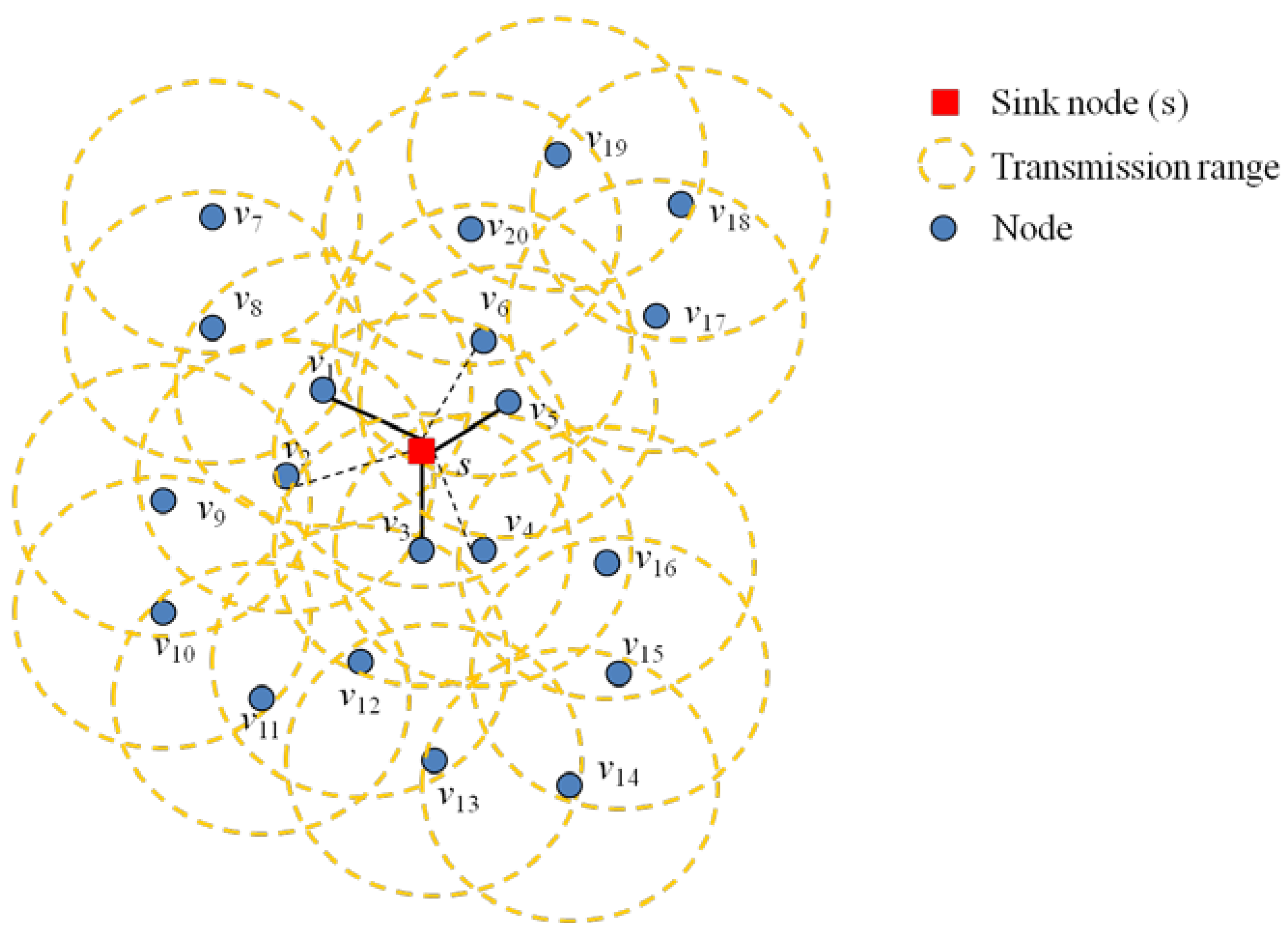
In step 1, the algorithm constructs the node set (Ns), which has nodes around the transmission range of the sink node (s). The algorithm selects a node that is closer to the sink node. 
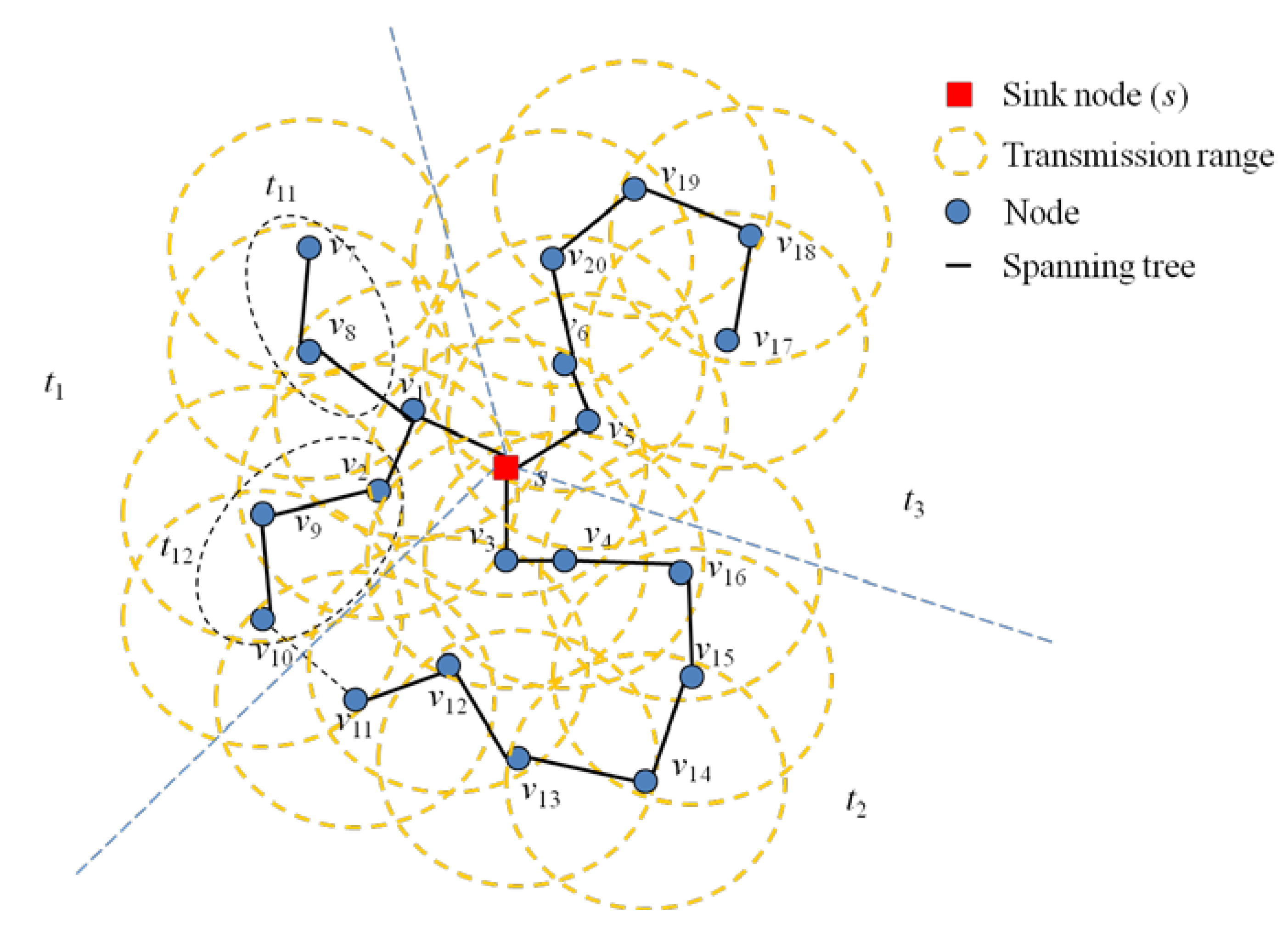
Figure 2 explains this step. The nodes, v1, v2, v3, v4, v5 and v6, are in the transmission range of the sink node, s. First, the algorithm needs to find a node set, Ns, from these nodes. If the algorithm finds that node v1 and v2 are in the range of the sink node, s, it calculates the weight from s to v1 and s to v2. Then, it selects the node, v1, which has the smaller weight than that of v2. The algorithm applies for the nodes, v3, v4, v5 and v6, and selects the nodes, v3 and v5, which have a smaller weight than those of v4 and v6. The complete set of nodes, Ns, is defined as follows:
Ns = {v1, v3, v5}
Figure 2. Node set (Ns) in the FMSTC algorithm (v1, v3 and v6, respectively, are chosen instead of v2, v4 and v5, because they are closer to the sink node (s)).
Algorithms 07 00145 g002
Once it has the complete set of nodes, Ns, it starts to construct the minimum spanning tree for each node in Ns that will be the root of each spanning tree. There are algorithms for constructing minimum spanning trees [9,10,17,28]. However, those algorithms are not suitable for WSNs, because WSNs are energy-constraint sensor networks. Therefore, we modified Khan’s algorithm, which is adaptable in WSNs, to get the minimum spanning tree from each node in Ns. Khan et al. [29] constructed a minimum spanning tree based on a rank function, which is decided by the random number and the unique id for each node. In this study, we use the weight of each distance instead of a random number, i.e., transmission range and node ids. The proposed algorithm constructs a minimum cost spanning tree; referred to as FMLSP (find minimum low cost spanning tree). Once the algorithm constructs all the minimum cost spanning trees, we assume that each of the trees is an independent set, i.e., each tree; there is no conflict to send a message because of the transmission range. The algorithm (referred to as FMLSP) is described in Table 2.
Table 2. FMLSP Algorithm
StepsProcedures
1All the nodes in the given network G = (V, E) have unique ids.
Select a node vi which has minimum number id from the given Ns set. Then put the node in the independent minimum spanning set ti, ti = {vi}.
Find all the neighboring nodes from vi.
  • If there exists only one neighboring node vj, which is within the transmission range, put the node in the independent minimum spanning tree ti, ti = {vi, vj}.
b.
If there exist more than two neighboring nodes within the transmission range, vj and vk, calculate the weights from vi to vj and vk, i.e. W(vj|vi) and W(vk|vi) (jk)
  • If W(vj|vi) is less than W(vk|vi), put the node vi to the independent minimum spanning set ti, ti = {vi, vj}, or vice versa, ti = {vi, vk}.
  • If W(vj|vi) is equal to W(vk|vi), put the node with smaller id number to the independent minimum spanning set ti.
c.
If there exists a node vm which is included in more than two independent minimum spanning trees, i.e. vmti and vmtj, calculate the weights from vm to vtia and vtjb, where vtiati and vtjbtj.
  • If W(vtia|vm) is less than W(vtjb|vm), put the node vm to the independent minimum spanning set ti, ti = {vi…, vm}, or vice versa, tj = {vj…, vm}.
  • If W(vtia|vm) is equal to W(vtjb|vm), put the node vm in the independent minimum spanning tree with smaller id number.
d.
Repeat (a) through (c) until it completes the construction of the independent minimum spanning tree for each node in Ns.
2While there exists a branch in the given independent minimum spanning tree ti, repeat Step 1(b) through 1(d) within the independent minimum spanning tree ti to construct the sub-tree tij.
The algorithm finds the minimum spanning tree set, ti, for each node in Ns. First, it finds all neighbor nodes in its transmission range. If two nodes are in the same transmission range, it calculates the weight for each link from a root node to a neighboring node. The algorithm selects the smaller weight to add to the node to the tree. If the weight of the link is the same for both of the nodes, the algorithm selects the node with the smaller id to add it to the tree. If the algorithm finds that a node is in the ranges of both of the trees, it measures a weight for each link and adds the node to the tree that has the smaller weight link. The algorithm also adds the node to the tree that has the smaller id if the weights of two links are the same in the case of a node that is in range of both of the trees. The algorithm repeats, until it gets the complete independent set of tree ti. After it gets a complete set of tree ti, it starts to find sub-tree set tij from ti. This process is for the next step of the FMSTC algorithm. The FMSTC algorithm builds the line topology after constructing a minimum spanning tree. This sub-tree set, tij, allows us to complete an independent set of tree ti by repeating the process described above. 
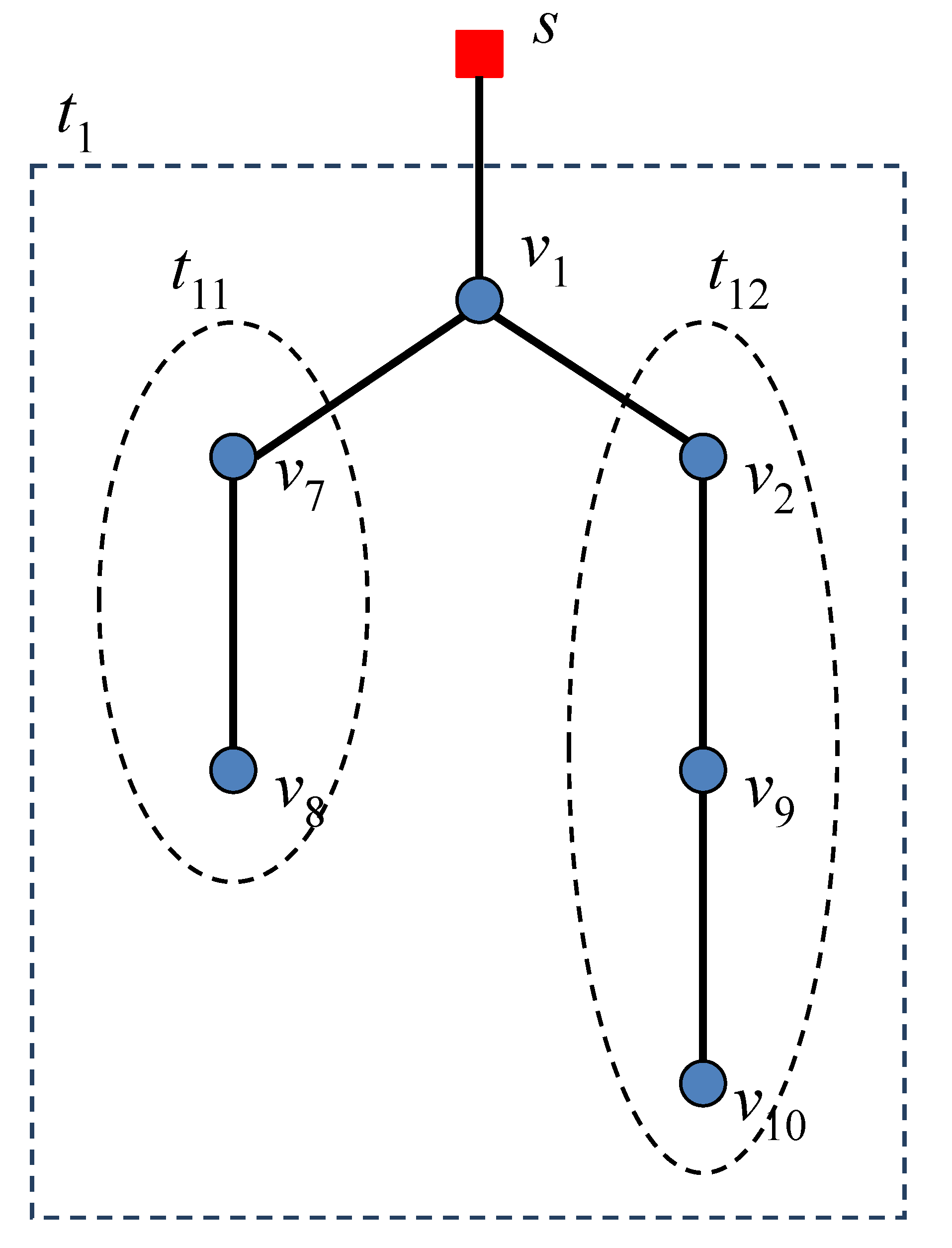
Figure 3 explains the sub-tree set environment.
Figure 3. Building a sub-tree set.
Algorithms 07 00145 g003
In Figure 3, the spanning tree, t1, has Nodes v1, v2, v7, v8, v9 and v10; t1 = {v1, v2, v7, v8, v9, v10}. A node, v1, is connected to sink node, and Nodes v2 and v7 are connected to v1. With a tree, t1, we can produce two sub-trees t11 = {v7, v8} and t12 = {v2, v9, v10}, i.e., t11t1 and t12t1.We eventually construct the line topology in the given minimum spanning tree set with this process. Figure 4 explains the algorithm to produce minimum spanning tree set ti. There are three minimum spanning trees: t1, t2 and t3.
Figure 4. Constructing the minimum spanning trees for nodes in the node set (Ns) using the FMLSP algorithm.
Algorithms 07 00145 g004
Three nodes (v1, v3, v5) are selected from a sink node. The FMSTC algorithm starts to construct a minimum spanning tree rooted from each node (v1, v3, v5). It produces three spanning trees, which are t1, t2 and t3. The tree, t1, has two leaf nodes, which need to be divided into two sub-spanning trees. The algorithm produces the sub-trees, t11 and t12, from t1. Therefore, there are five spanning trees produced in the graph:
t1 = {v1, v2, v7, v8, v9, v10}; t11 = {v7, v8}, t12 = {v2, v9, v10}
t2 = {v3, v4, v11, v12, v13, v14, v15, v16}
t3 = {v5, v6, v17, v18, v19, v20}
the node, v10, is in the spanning tree, t12, because it is close to Node v9, even though it is also in the transmission range of v11, which is in t2.

4.2. Applying Linear Structure to Get the Minimum Scheduling Time for Convergecast

The algorithm produces the line structure of each spanning tree. We applied the algorithm of Choi et al. [3] to get the minimum scheduling time. The authors have proposed an optimal convergecast scheduling algorithm based on the line topology with a fixed transmission range. The developed algorithm consists of four different algorithms. When the number of sensors is in a range less than the transmission range, the SIMPLE algorithm is used to send a message to the sink node directly. If the number of sensors is placed in the pnp(p + 1) range, where n is the number of sensors and p is the transmission power, then apply the TABLE and ADJUST algorithms. If the number of sensors is placed in the p (p + 1) < n range, then apply the REDUCE algorithm first to use TABLE and ADJUST. The algorithms, SIMPLE, TABLE, ADJUST and REDUCE, are described in more detail as follows:
(1) If n < p, then apply the SIMPLE algorithm, which can allocate n time slots for the messages (mi, 1 ≤ in) to send a message from node i to the sink node at time slot i, because each node directly sends the message to the sink node in the given condition.
(2) If pnp(p + 1), then apply the TABLE and ADJUST algorithms. The TABLE algorithm allows us to allocate 2p(p + 1) − p time slots to deliver any p(p + 1) messages; on the other hand, the ADJUST algorithm reallocates it for p(p + 1) nodes and then allocates the time slots for n nodes.
(3) If p(p + 1) < n, then apply the REDUCE algorithm with (np) nodes and then apply the TABLE and ADJUST algorithms.
Table 3 explains the minimum time schedule for using these algorithms.
Table 3. Time schedule with TABLE when n = 10, p = 3.
TimeNode
012345678910
1040000001100
2005000000120
3000600000013
410000800000
520000090000
6300000010000
7400001100000
8500000120000
9600000013000
10008000000150
11000900000016
120011000000180
130001200000019
14800000150000
15900000016000
161100000180000
171200000019000
18000150000000
19000180000000
20150000000000
21180000000000
2200000000000
2300000000000
2400000000000
The above table is the output of the TABLE algorithm and function TABLE, with 11 nodes, including the sink node and three transmission ranges. We want to deliver the individual contents to the sink node, where the content number is the message originating from the cell number. The algorithms assumed that they can use virtual nodes, which are not physically used. The virtual node numbers used in this algorithm are {11, 12, 13, 15, 16, 18, 19}. In the table, the content “0” means there is no message delivered at the assigned time slot. For example, for the node number “1” and time slot “1”, there is content from the node “4”. For the node number “8” and time slot “1”, there is content from the node “11”, which is the virtual node.
When we send Contents 4, 5 and 6 to Nodes 1, 2 and 3, we move the non-conflicting messages in the same time slot as follows:
When sending 4 to 1, then move 11 to 8, and 18 to 15, and so on, up to n + p2 (here, 10 + 9 = 19);
when sending 5 to 2, then move 12 to 9 and 19 to 16, when sending 6 to 3; then move 13 to 10.
When we send Contents 1, 2 and 3 to the sink node, we also move the non-conflicting messages in the same time slot as follows:
When sending 1 to the sink node (0), then move 8 to 5 and 15 to 12;
when sending 2 to the sink node (0), then move 9 to 6 and 16 to 13;
when sending 3 to the sink node (0), then move 10 to 7.
When we send Contents 4, 5 and 6 to the sink node, we move non-conflicting messages as follows:
When sending 4 to 1, then move 11 to 5 and 18 to 12;
when sending 5 to 1, then move 12 to 6 and 19 to 13;
when sending 6 to 1, then move 13 to 7.
When we send Contents 8 and 9 to Nodes 2 and 3, we can move 15 to 9 and 16 to 10.
When we send Contents 11 and 12 to Nodes 2 and 3, we can move 18 to 9 and 19 to 10.
When we send Contents 8 and 9 to the sink node, we can move 15 to 6 and 16 to 7.
After we send Content 15 to 3 in time slot 18 and 18 to 3 in time slot 19, Contents 15 and 18 arrive at the sink node in Time Slots 20 and 21.
Table 4 is made, and it has p(p + 1) messages in the sink node, because n is always less than or equal to p(p + 1).
Table 4. Time schedule with ADJUST − (1) when n = 10, p = 3.
TimeNode
012345678910
1040000001100
2005000000120
3000600000013
410000800000
520000090000
6300000010000
7400001100000
8500000120000
9600000013000
10008000000150
11000900000016
120011000000180
130001200000019
14800000150000
15900000016000
161100000180000
171200000019000
18000150000000
19000180000000
20150000000000
21180000000000
2200000000000
2300000000000
2400000000000
In the sink node, we have messages, i.e., 1, 2, 3, 4, 5, 6, 8, 9, 11, 12, 15 and 18. That means we missed Messages 7 and 10. For 7, we find the smallest number, but greater than n (=10), among those received, which is 11.
After searching 11 among Column 7, 6 and 5, we can find it at Table (7, 5) and replace the content with 7. The next 11 is located in column 2 (5 − 3 = 2) which is the Table (12, 2), and we replace the content with 7. The next, 11, is located in 0 (2 − 3 = −1, but the negative number is always 0 here), which is the Table (0, 16); replace Table (0, 16) with 7. We can execute the same algorithm for the content of 10. Then, we can get Table 5.
Table 5. Time schedule with ADJUST − (2) when n = 10, p = 3.
TimeNode
012345678910
1040000001100
2005000000100
3000600000013
410000800000
520000090000
6300000010000
740000700000
8500000100000
9600000013000
10008000000150
11000900000016
12007000000180
130001000000019
14800000150000
15900000016000
16700000180000
171000000019000
18000150000000
19000180000000
20150000000000
21180000000000
2200000000000
2300000000000
2400000000000
The next step of the algorithm deletes all numbers greater than n and deletes all rows that do not contain any number from one to n. Table 6 shows the minimum time schedule when the number of nodes n = 10 and the transmission range p = 3.
Table 6. Completed time schedule when n = 10, p = 3.
TimeNode
012345678910
1040000001100
2005000000100
300060000000
410000800000
520000090000
6300000010000
740000700000
8500000100000
960000000000
1000800000000
1100090000000
1200700000000
13000100000000
1480000000000
1590000000000
1670000000000
17100000000000
The example we used is when the number of nodes is less than p (p + 1), n < p(p + 1). If the number of nodes is greater than p(p + 1), n > p(p + 1), the REDUCE algorithm is applied to make the condition, n < p(p + 1); then, use the TABLE and ADJUST algorithm to get the minimum time schedule. For example, If n = 14 and p = 3, we have nodes, n = {1, 2, 3, 4, 5, 6, 7, 8, 9, 10, 11, 12, 13, 14}; then, make it n = {4, 5, 6, 7, 8, 9, 10, 11, 12, 13, 14} using Table 7, as follows.
Table 7. Time schedule with REDUCE when n = 14, p = 3.
TimeNode
01234567891011121314
11----8---------
22-----9--------
33------10-------
4-4------11------
5--5------12-----
6---6------13----
7----7------14---
After 2p + 1 = 7 steps, we have n = {4, 5, 6, 7, 8, 9, 10, 11, 12, 13, 14}. This is the same as the problem with n = 10 and p = 3 from this point. Then, we use the TABLE and ADJUST algorithms to get the minimum time schedule.

5. Simulation and Results

In this section, we evaluate the performance of our proposed algorithm (FMSTC) by numerical simulation. The simulation is programmed in Visual C++ language. We produced the connected network graphs by randomly distributing nodes in a 500 × 500 square board. We considered the networks with various numbers of nodes, i.e., 10, 20, 30, 40, 50, 60, 70, 80, 90 and 100 nodes. The power range (or transmission range) was fixed before the simulation was started, and different power ranges were considered. Here, we used the following power ranges: three, six, nine, 12 and 15 units. Once the simulation is started, a sink node is randomly selected. As mentioned in an earlier section, other researchers have tried to solve the convergecast problem. However, most of them make different assumptions and take different approaches than ours. No direct comparison with their work is possible. We first report the number of time slots required by the proposed algorithm and then represent the results, which are compared to the optimal scheduling algorithm in the linear topology developed by Choi et al. [3]. In Section 5.1, we show the results of the optimal solution for a linear topology. The simulation results of the proposed algorithm for the convergecast scheduling time in the general topology were shown in detail in Section 5.2. The performance evaluation follows in Section 5.3.

5.1. Optimal Solution for a Linear Topology

As we stated in the previous section, Choi et al. [3] proposed the optimal scheduling algorithm for convergecast in a linear network topology with a fixed transmission range, and we have applied their algorithm to a general network topology to get the minimum scheduling time. Their algorithm produces n times if n < p, 2np time if pnp(p + 1) and 2n − 2p + n / p –1 time if n > p(p + 1), where p is power (=transmission range). In this section, we show the minimum time if the given number of nodes are in a linear topology. Table 8 and Figure 5 represent the optimal time schedule for the given number of nodes in a linear network topology with fixed power.
Table 8. Optimal time schedule in a linear topology with fixed power.
PowerNumber of Nodes
102030405060708090100
317.0039.6763.0086.33109.67133.00156.33179.67203.00226.33
614.0034.0054.0074.0095.33117.00138.67160.33182.00203.67
911.0031.0051.0071.0091.00111.00131.00151.00171.00192.11
1210.0028.0048.0068.0088.00108.00128.00148.00168.00188.00
1510.0025.0045.0065.0085.00105.00125.00145.00165.00185.00
As Table 8 illustrates, when the power is three and 10 nodes are placed on the line, it needs 17 time slots. If 100 nodes are placed, it needs 226.33 time slots, which is the maximum. As the power is increased, time slots are decreased, as is shown in Figure 5. When the power is 12 or 15, the time slots are 10 with 10 nodes, because the number of nodes are less than the power (n < p).
Figure 5. Optimal scheduling time in a linear topology with fixed power.
Algorithms 07 00145 g005

5.2. Scheduling Time for Convergecast in General Topology

Each simulation experiment for getting the scheduling time for convergecast in a general topology was repeated 30 times based on the number of nodes, and the average values of all trials for each are reported. The simulation displays randomly distributed nodes. The FMSTC algorithm chooses nodes that are closer to the sink node. It shows a fully connected graph and constructs the minimum spanning trees, which are independent sets to get the line topologies. Additionally, it starts sending messages to the sink node. Figure 6 is an example of the simulation.
Figure 6. (a) 40 sensors distribution with p = 3; (b) 50 sensors distribution with p = 3. Example of the simulation: 1, node distribution; 2, fully connected graph based on chosen nodes near the sink node; 3, constructing minimum spanning trees.
Algorithms 07 00145 g006
As shown in Figure 6a (1), 40 nodes are distributed in a 500 × 500 square area. We set up the transmission range to three units. After deciding on the sink node, the nodes construct the fully connected graph based on the chosen nodes near the sink node in Figure 6a (2). Finally, the nodes in the square area can construct the minimum spanning tree using our proposed algorithm (FMLSP), as shown in Figure 6a (3). We present the results of the overall simulation in Table 9 and Figure 7.
As shown in Figure 7, the more nodes, the more time slots in each power level. When the power is increased, the time slots decrease. Some of the time slots are increased by a greater number. For example, time slots increased more than 100, from 60 nodes to 70 nodes, for Power Levels 6, 9 and 12. This increase is due to the fact that more sub-spanning trees are made during the simulation. That means that the proposed algorithm may generate more branches when the node number is increased.
Figure 7. Scheduling time for convergecast in the general topology.
Algorithms 07 00145 g007
Table 9. Scheduling time in the general topology.
PowerNumber of Nodes
102030405060708090100
355.00115.23165.23199.33285.53335.40422.50493.43530.63588.93
645.53103.77156.43185.83258.27297.57398.17458.17490.73531.30
930.8396.80143.23180.50230.77286.93387.57448.10480.57514.37
1229.5375.77135.70171.17224.50276.43382.87435.70471.30512.17
1523.2056.13120.53153.67194.17267.97355.97416.23459.00503.13

5.3. Performance Evaluation

The performance is evaluated by comparing FMSTC scheduling time to scheduling time in a linear topology (scheduling time is optimal in a linear topology). Figure 8 shows the relationship between power, the number of nodes and optimal time slots in a linear topology.
Figure 8. Power vs. the number of nodes vs. optimal time slots in a linear topology.
Algorithms 07 00145 g008
We notice that the number of time slots required increases as the number of nodes is increased and the allocated power is decreased, as shown in Figure 8. Notice that the number of time slots is increased monotonically with respect to the variations of power and node numbers. Figure 9 shows the relationship among power, the number of nodes and time slots in the general topology.
Figure 9. Power vs. number of nodes vs. time slots in the general topology.
Algorithms 07 00145 g009
We notice that the number of time slots required in the general topology is increased as the number of nodes increases and the allocated power decreases, as shown in Figure 9. Be aware that there exists a little bit of a steep increase between nodes Number 60 and 70, due to the additional sub-spanning trees made during the simulation. This steep increase, however, does not affect the overall performance of scheduling allocation with respect to the linear topology. We will show that in the following table.
Table 10 represents the ratio with the result of the simulation and the optimal scheduling time in the linear topology.
Table 10. Ratio with the simulation result (The number of time slots in FMSTC/The number of time slots in optimal).
PowerNodeAverage
102030405060708090100
33.242.912.622.312.602.522.702.752.612.602.69
63.253.052.902.512.712.542.872.862.702.612.80
92.803.122.812.542.542.582.962.972.812.682.78
122.952.712.832.522.552.562.992.942.912.722.77
152.322.252.682.362.282.552.852.872.782.722.57
-2.72
As shown in Table 10, when the power is three with 10 nodes, the ratio is 3.24, meaning that in the general topology, it needs 3.24 times more time slots than the linear topology to get all the messages from each node. The average of the ratio is 2.69 when the power is three, 2.80 when the power is six, 2.78 when the power is nine, 2.77 when the power is 12 and 2.57 when the power is 15. The average ratio for the scheduling times of the steep increase is 2.55 for node Number 60 and 2.87 for node Number 70, respectively.
The ratio difference is negligible, as is shown in Table 10. The highest ratio is when the power is six with 10 nodes (3.25), and the lowest ratio is when the power is 15 with 50 nodes (2.28). The overall average ratio is 2.72.

6. Conclusion

In this work, we studied the convergecast problem for a general network topology with fixed transmission power in a wireless sensor network. We first proposed the scheduling algorithm (FMSTC) to find the minimum time slots for convergecast in a general topology using a line- and tree-based topology and evaluated the performance of our approach by the simulations. The results of the simulation showed that when the power is increased, the time slots decreased. The maximum time slot is 588.93 with 100 nodes when the power is three, and the minimum time slot is 23.20 with 10 nodes when the power is 15. We have compared our simulation results to the optimal time slots in the linear network topology. The highest ratio was 3.25 when the power was fixed to six with 10 nodes, and the lowest ratio was 2.28 when the power was fixed to 15 with 50 nodes. The results showed that the convergecast in the general topology has more than twice the time slots compared to the linear topology. The overall ratio was 2.27, which means that the proposed algorithm (FMSTC) for convergecast in the general network topology has 2.27 times more time slots than that of the linear network topology.
In this study, we showed that the linear network topology that gets the optimal scheduling time can be extended to the general network topology to get the minimum scheduling time. The result of this study is extracted from an iterative trial of the simulation. To our best knowledge, the proposed method is the first trial to apply the use of the optimal algorithm in a linear network topology to a general network topology. This study showed that the average number of required time slots for a general topology is less than 2.27 times the number of required time slots for a linear topology. This result is the best minimum scheduling time for a general topology known so far.

Conflicts of Interest

The authors declare no conflict of interest.

References

  1. Ghosh, A.; Incel, O.D.; Kumar, V.S.A.; Krishnamachari, B. Multi-Channel Scheduling Algorithms for Fast Aggregated Convergecast in Sensor Networks. In Proceedings of the IEEE 6th International Conference on Mobile Adhoc and Sensor Systems, Macau, China, 12–15 October 2009; pp. 363–372.
  2. Kumar, S.; Chauhan, S. A survey on scheduling algorithms for wireless sensor networks. Int. J. Comput. Appl. 2011, 20, 7–13. [Google Scholar]
  3. Choi, H.; Yang, S.; Kim, Y.; Joo, H. On the Scheduling for Convergecast in Power Controlled Wireless Sensor Networks. In Proceedings of the IEEE ICCCN Workshop, Arlington, UT, USA, 31 July 2011.
  4. Choi, H.; Wang, J.; Hughes, E. Schduling for Information Gathering on Sensor Network. In Wireless Networks; Springer: Berlin, Germany, 2009; Volume 15, pp. 127–140. [Google Scholar]
  5. Annamalai, V.; Gupta, S.; Schwiebert, L. On tree-based convergecasting in wireless sensor networks. In Proceedings of the IEEE Wireless Communications and Networking Conference (WCNC), New Orleans, LA, USA, 20 March 2003; pp. 1942–1947.
  6. Bechkit, W.; Koudil, M.; Challal, Y.; Bouabdallah, A.; Souici, B.; Benatchba, K. A New Weighted Shortest Path Tree for Convergecast Traffic Routing in WSN. In Proceedings of the 2012 IEEE Symposium on Computers and Communications (ISCC), Washington, DC, USA, 2012; pp. 187–192.
  7. Gandham, S.; Zhang, Y.; Huang, Q. Distributed Minimal Time Convergecast Scheduling in Wireless Sensor Networks. In Proceedings of the 26th IEEE International Conference on Distributed Computing Systems, Lisboa, Portugal, 4–7 July 2006; pp. 1–50.
  8. Incel, O.D.; Ghosh, A.; Krishnamachari, B.; Chintalapudi, K. Fast data collection in tree-based wireless sensor networks. IEEE Trans. Mob. Comput. 2012, 11, 86–99. [Google Scholar] [CrossRef]
  9. Li, X.; Wang, Y.; Wan, P.; Song, W.; Feieder, O. Localized Low-Weight Graph and its Application in Wireless Ad Hoc Networks. In Proceedings of the IEEE INFOCOM, Chicago, IL, USA, 7–11 March 2004.
  10. Peleg, D. Distributed Computing: A Locality-Sensitive Approach; SIAM: Philadelphia, PA, USA, 2000. [Google Scholar]
  11. Ramanathan, S.; Llyod, E.L. Scheduling algorithms for multihop radio networks. IEEE/ACM Trans. Netw. 1993, 1, 166–177. [Google Scholar] [CrossRef]
  12. Sinem, E.; Pravin, V. TDMA scheduling algorithms for wireless sensor networks. Wirel. Netw. 2010, 16, 985–997. [Google Scholar]
  13. Gandham, S.; Dawande, M.; Parkash, R. Link scheduling in sensor networks: Distributed edge coloring revisited. J. Parallel Distrib. Comput. 2008, 68, 1122–1134. [Google Scholar] [CrossRef]
  14. Zhang, H.; Soldati, P.; Johansson, M. Optimal Link Scheduling and Channel Assignment for Convergecast in Linear Wireless HART Networks. In Proceedings of the 7th International Symposium on Modeling and Optimization in Mobile, Ad Hoc, and Wireless Networks, Seoul, Korea, 23–27 June 2009; pp. 1–8.
  15. Suh, C.; Shin, J.; Lee, J. Fusion Rate Based Spanning Tree. In Proceedings of the 11th IEEE Singapore International Conference on Communication Systems, Seoul, Korea, 19–21 November, 2008; pp. 1721–1726.
  16. Tsai, H.; Chen, T. Minimal Time and Conflict-Free Schedule for Convergecast in Wireless Sensor Networks. In Proceedings of IEEE International Conference on Communications, Beijing, China, 19–23 May 2008; pp. 2808–2812.
  17. Ahuja, R.K.; Magnanti, T.L.; Orlin, J.B. Network Flows-Theory, Algorithms, and Applications; Prentice Hall: Upper Saddle River, NJ, USA, 1993; Chapter 4. [Google Scholar]
  18. Malhortra, B.; Nikolaidis, I.; Nascimento, M.A. Aggregation convergecast scheduling in wireless sensor networks. Wirel. Netw. 2011, 17, 319–335. [Google Scholar] [CrossRef]
  19. Luo, D.; Zhu, X.; Wu, X.; Chen, G. Maximizing Lifetime for the Shortest Path Aggregation Tree in Wireless Sensor Networks. In Proceedings of the IEEE INFOCOM, Nanjing, China, 10–15 April 2011; pp. 1566–1574.
  20. Gomez, J.; Campbell, A.T. Variable-range transmission power control in wireless ad hoc networks. IEEE Transactions Mob. Comput. 2007, 6, 87–99. [Google Scholar] [CrossRef]
  21. Kawadia, V.; Kumar, P.R. Principles and protocols for power control in wireless ad hoc networks. IEEE J. Sel. Areas Commun. 2005, 23, 76–88. [Google Scholar] [CrossRef]
  22. ElBatt, T.; Ephremides, A. Joint scheduling and power control for wireless ad hoc networks. IEEE Transactions Wirel. Commun. 2004, 3, 74–85. [Google Scholar] [CrossRef]
  23. Kesselman, A.; Kowalski, D. Fast Distributed Algorithm for Convergecast in Ad Hoc Geometric Radio Networks. In Proceedings of the Second Annual Conference on Wireless on Demand Network Systems and Services (WONS), St. Moritz, Switzerland, 19–21 January 2005; pp. 119–124.
  24. Huang, Q.; Zhang, Y. Radial Coordination for Convergecast in Wireless Sensor Networks. In Proceedings of the 29th Annual IEEE Internaitonal Conference on Local Computer Networks (LCN), Tampa, FL, USA, 16–18 November 2004; pp. 542–549.
  25. Vergados, D.J.; Manolaraki, M.-Y.; Vergados, D.D. Evaluation of Broadcast Scheduling Algorithm for Ad-hoc TDMA Networks. In Proceedings of the ITAE, Aalborg, Greece, 17–20 May 2009; pp. 17–20.
  26. Xu, K.; Gerla, M.; Bae, S. Effectiveness of RTS/CTS handshake in IEEE 802.11 based ad hoc networks. Ad hoc Networks 2003, 1, 107–123. [Google Scholar] [CrossRef]
  27. Zhou, G.; He, T.; Stankwic, J.; Abdelzaher, T. RID: Radio Interference Detection in Wireless Sensor Network. In Proceedings of the INFOCOM, Charlottesville, VA, USA, 13–17 March 2005; pp. 891–901.
  28. Li, X. Algorithmic, Geometric and graphs issues in wireless networks. J. Wirel. Comm. Mob. Comput. 2003, 3, 119–140. [Google Scholar] [CrossRef]
  29. Khan, M.; Pandurangan, G.; Kumar, V.S.A. Distributed algorithms for constructing approximate minimum spanning trees in wireless sensor networks. IEEE Trans. Parallel Distrib. Syst. 2009, 20, 124–139. [Google Scholar] [CrossRef]

