Modeling Dynamic Programming Problems over Sequences and Trees with Inverse Coupled Rewrite Systems

Abstract

Dynamic programming is a classical algorithmic paradigm, which often allows the evaluation of a search space of exponential size in polynomial time. Recursive problem decomposition, tabulation of intermediate results for re-use, and Bellman’s Principle of Optimality are its well-understood ingredients. However, algorithms often lack abstraction and are difficult to implement, tedious to debug, and delicate to modify. The present article proposes a generic framework for specifying dynamic programming problems. This framework can handle all kinds of sequential inputs, as well as tree-structured data. Biosequence analysis, document processing, molecular structure analysis, comparison of objects assembled in a hierarchic fashion, and generally, all domains come under consideration where strings and ordered, rooted trees serve as natural data representations. The new approach introduces inverse coupled rewrite systems. They describe the solutions of combinatorial optimization problems as the inverse image of a term rewrite relation that reduces problem solutions to problem inputs. This specification leads to concise yet translucent specifications of dynamic programming algorithms. Their actual implementation may be challenging, but eventually, as we hope, it can be produced automatically. The present article demonstrates the scope of this new approach by describing a diverse set of dynamic programming problems which arise in the domain of computational biology, with examples in biosequence and molecular structure analysis.

1. Introduction

• Mapping from concrete to abstract
• is always the easier way.
Harald Ganzinger

1.1. Motivation

In the field of biosequence analysis, combinatorial optimization problems on sequences and trees arise in never-ending variety. These problems include string comparison, prediction and comparison of molecular structures, pattern matching in trees and forests, and modeling of families of related sequences or structures. Often, there is a prototypical algorithm, which is based on the dynamic programing paradigm [1] and must be adapted to different applications. Let us skim over the domains from which we draw the algorithmic problems described in this manuscript.

For determining similarity in genes and proteins, there is the “Needleman-Wunsch” alignment algorithm, refered to as “string edit distance” in the broader field of computer science [2,3]. It is used with a variety of scoring schemes that differ in their treatment of matches and mismatches, in their modeling of gaps, and by either minimizing distance or maximizing similarity. Equally famous in bioinformatics is the “Smith-Waterman” algorithm for finding most conserved sub-sequences in genes and proteins [4], also refered to as the “local similarity” algorithm. It is derived from string edit distance by allowing the algorithm to skip prefixes and suffixes of both sequences free of charge. Except for minimizing distance (which makes no sense with local similarity), local similarity comes with the same variants as global string edit distance. Then, there are hybrids of both algorithms: Matching a complete sequence to a sub-sequence of a longer one, or “free shift” alignment, where one sequence may be displaced with respect to the other, but else, a global distance or similarity is sought. When searching sequence databases, one of the two inputs may be fixed, giving rise to a (potentially faster) matching algorithm. In all applications, sometimes we only ask for a similarity or distance score, sometimes we want an optimal alignment which justifies this score, and sometime we even want to obtain all near-optimal alignments up to some score threshold, to perform further analysis on them.

Analysis of structural RNAs is also a source of algorithmic problems. RNA structure prediction is achieved by dynamic programming algorithms, based on stochastic or thermodynamic models. Again, one asks for optimal or near-optimal structures, for good local structures, for structures that match a given model structure, and so on. A more sophisticated problem is addressed by the Sankoff algorithm [5], which predicts an optimal consensus structure for two RNA molecules. On a very abstract level, one could say that this algorithm uses two instances of the RNA folding algorithm and one instance of sequence alignment simultaneously and with a joint optimization objective. Ideas from string comparison are re-used in a more general form in the comparison of structures. RNA secondary structures are naturally represented as ordered, rooted trees. On trees and forests, a familiar set of problem variants arises. Edit distance and alignment are slightly different problems on trees. Again, we ask for distance/similarity, local/global comparison, atomic/composite gaps, optimal/near-optimal solutions, and we may be interested only in the optimal score or also in the underlying alignment. Where hidden Markov models describe sequence families, families of structures are described by covariance models, a special form of stochastic context-free grammars.

While there is much re-use of algorithmic ideas in combinatorial optimization problems on trees and sequences, this is not transparent in the way we represent concrete algorithms. Their formulation as dynamic programming algorithms requires us to integrate all problem aspects–construction of the search space, scoring, tabulation of intermediate results, and reporting one or more solutions. This leads to algorithms with a low level of abstraction, and to programs that are non-trivial to write, tedious to debug, and delicate to modify. Code reliability and code re-use suffer from this low level of abstraction. With new problem variants, it is often not clear at the outset how the search space should be modeled and how the objective function should be defined in detail. It would be advisable to experiment with different approaches, but the high implementation effort prevents this.

1.2. Overview

We introduce Inverse Coupled Rewrite Systems (ICOREs) as a high-level and unified view on a diverse set of combinatorial optimization problems on sequences and trees. ICOREs are based on the following ideas: Candidate solutions of optimization problems have a natural representation in some term algebra, whose function symbols reflect the case analysis required by the problem at hand. A tree grammar may be used to further refine the search space by describing a language of well-formed candidates. Optimization objectives are specified as interpretations of these terms in a suitable scoring algebra, together with an objective function. The relation between input terms and their candidate solutions is established by a term rewrite system. This rewrite system works in the wrong direction, mapping solutions back to the input(s) of the problem they solve. For problems with several inputs, the rewriting to these inputs is performed by different rules, but in a coupled manner.

These constituents provide a mathematically precise and complete problem specification. Implementing an algorithm to solve the problem is non-trivial. To actually solve a problem for given inputs, the coupled rewrite relation must be inverted. Candidates must be constructed, evaluated, and have the objective applied to them. To do so efficiently, all the dynamic programming machinery must eventually be brought in—but no allusion to dynamic programming appears in the problem specification.

The goal of such work is twofold. One wants to

• describe optimization problems on a declarative level of abstraction, where fundamental ideas are not obscured by implementation detail, and relationships between similar problems are transparent and can be exploited;
• implement algorithmic solutions to these problems in a systematic or even automated fashion, thus liberating algorithm designers from error-prone coding and tedious debugging work, enabling re-use of tried-and-tested components, and overall, enhancing programmer productivity and program reliability.

In the present manuscript, we focus on the former of these goals. We will develop a substantial number of problem specifications expressed in our new framework, all drawn from the application domains of computational biology. However, as much as sequences, trees and dynamic programming are ubiquitous in computer science, this article covers only a small sub-domain of the potential scope of our approach. For example, the tree comparison techniques we use with RNA secondary structure have also been employed to compare objects assembled by robots, or to extract and compare documents from the web [6,7]. By presenting a diverse set of real-world examples from bioinformatics, we are hoping to convince the reader that the second goal, developing implementation techniques for ICOREs, is a new and rewarding research challenge.

1.3. Previous Work

Quite early in the young field of bioinformatics, researchers have advocated general techniques for specifying and implementing such algorithms. In a series of papers, Searls introduced the use of concepts from formal language theory palwith problems in biosequence analysis [8,9,10]. In particular, context free grammars were advocated for molecular pattern matching, and letter transducers were introduced to model problems related to string edit distance of DNA sequences. This work has been very influential in attracting computer scientists to the problems of biosequence analysis, but has not led to competitive implementation techniques. Not much later, Lefebvre advocated the use of s-attributed grammars [11]. He showed that not only sequence comparison, but also complex problems such as simultaneous alignment and folding of two RNA sequences (introduced above as the Sankoff algorithm [5]) can be described by grammars and solved by a suitable (generated) parsing algorithm. However, s-attributed grammars are the most restricted class of attribute grammars [12], offering little more advantage than amalgamating construction of a parse tree with its evaluation by structural recursion. Maybe because of this limitation and the notational overhead that comes with attribute grammars, this work has received less interest in the bioinformatics community than it may have deserved.

Algebraic dynamic programming (ADP) [13] provides a declarative approach to dynamic programming problems over sequence data. It goes beyond the aforementioned approaches by enhancing grammar-based descriptions with an algebraic semantics, allowing to formally model not only search space construction, but also its evaluation under varying objectives. Several implementations of ADP as a domain-specific language for dynamic programming over sequence data have been developed [14,15,16].

In Section 9, after we have laid out our new framework and have explored its range of applications, we will explicitly relate our ideas to Searls’ letter transducers and Lefebvre’s s-attributed grammars. We will also show that the new framework properly generalize the present ADP framework, and will argue that it even improves its intuitive appeal.

1.4. Article Organization

This article is organized as follows. Section 2 shows a first application example, even before the formal definitions are given. In Section 3, we collect technical definitions which are familiar from the literature. Readers with a strong background in these concepts may skip their formal exposition and jump right ahead. In Section 4, we formally introduce ICOREs. We suggest a pseudocode notation for writing ICOREs, add some notational conventions, and offer an ICORE design exercise to the reader. Then, we proceed to model various problems in biosequence and structure analysis. Section 5 discusses sequence comparison problems in various guises, Section 6 deals with folding RNA sequences into a secondary structure and related problems such as stochastic RNA family models, and Section 7 focuses on several variants of tree comparison and pattern matching. Table 1 summarizes the ICOREs presented in this manuscript. Curious readers are invited to skip all the technicalities and take a look ahead, to see how the problem they are most familiar with is dressed up as an ICORE. While Section 5, Section 6 and Section 7 are concerned with the construction of the search spaces for various problem types, Section 8 deals with the evaluation of search spaces, including the combined use of several scoring schemes and objective functions. In Section 9, we relate ICOREs to the present state-of-the-art in implementing algebraic dynamic programming, and to other computational models from older work. In the Conclusion, we review some design decisions that were made with this first exposition of ICOREs, and discuss the challenges of ICORE implementation.

Table 1. A summary of the Inverse Coupled Rewrite Systems (ICOREs) presented in this manuscript. In a few cases, not a complete ICORE is specified, but only a grammar that extends another ICORE.

ICORE/Grammar	Dim.	Problem addressed	In Section	Page
EditDistance	2	simple edit distance/alignment	4.2	77
Affine	2	edit distance, affine gaps	5.1	82
AffiOsci	2	oscillating affine gaps	5.1	84
AffiTrace	2	sequence traces, affine gaps	5.1	84
LocalSearch	2	generic local alignment	5.2	85
MotifSearch	2	short in long alignment	5.2.1.	86
SemiGlobAlignment	2	semi-global alignment	5.2.2.	86
LocalAlignment	2	local alignment	5.2.3.	86
MatchSeq_S	1	hardwired sequence matching	5.3.1.	88
MatchAffi_S	1	same with affine gap model	5.3.1.	88
MatchSeq_S	1	profile HMM	5.3.2.	88
with position-specific scores
RNAfold	1	RNA folding	6.3	93
StructAli	2	struct. Alignment prototype	6.4	97
SimultaneousFolding	2	generalized fold and align	6.5	98
ExactConsensusStructure	2	exact consensus structure	6.5.2.	98
		for two RNA sequences
Sankoff	2	simultaneous fold and align	6.5.3.	99
S2SGeneric	2	covariance model, generic	6.6.1.	101
S2SExact	2	match RNA sequence	6.6.2.	100
		to target structure
Match_S2S_r	2	exact local motif matcher	6.6.4.	103
Match_S2S_r’	1	motif matcher, hard coded	6.6.4.	104
SCFG	1	stochastic context free grammar	6.3	93
CovarianceModel_r	1	covariance model, hard coded	6.6.5.	106
TreeAlign	2	classical tree alignment	7.2	111
TreeAliGeneric	2	tree alignment protoype + variants	7.2.2.	113
OsciSubforest	2	tree ali. with oscillating gaps	7.2.2.	117
TreeEdit	2	classical tree edit	7.3	119
RNATreeAli	2	RNA structure alignment	7.5	127

Table 1. A summary of the Inverse Coupled Rewrite Systems (ICOREs) presented in this manuscript. In a few cases, not a complete ICORE is specified, but only a grammar that extends another ICORE.

ICORE/Grammar	Dim.	Problem addressed	In Section	Page
EditDistance	2	simple edit distance/alignment	4.2	77
Affine	2	edit distance, affine gaps	5.1	82
AffiOsci	2	oscillating affine gaps	5.1	84
AffiTrace	2	sequence traces, affine gaps	5.1	84
LocalSearch	2	generic local alignment	5.2	85
MotifSearch	2	short in long alignment	5.2.1.	86
SemiGlobAlignment	2	semi-global alignment	5.2.2.	86
LocalAlignment	2	local alignment	5.2.3.	86
MatchSeq_S	1	hardwired sequence matching	5.3.1.	88
MatchAffi_S	1	same with affine gap model	5.3.1.	88
MatchSeq_S	1	profile HMM	5.3.2.	88
with position-specific scores
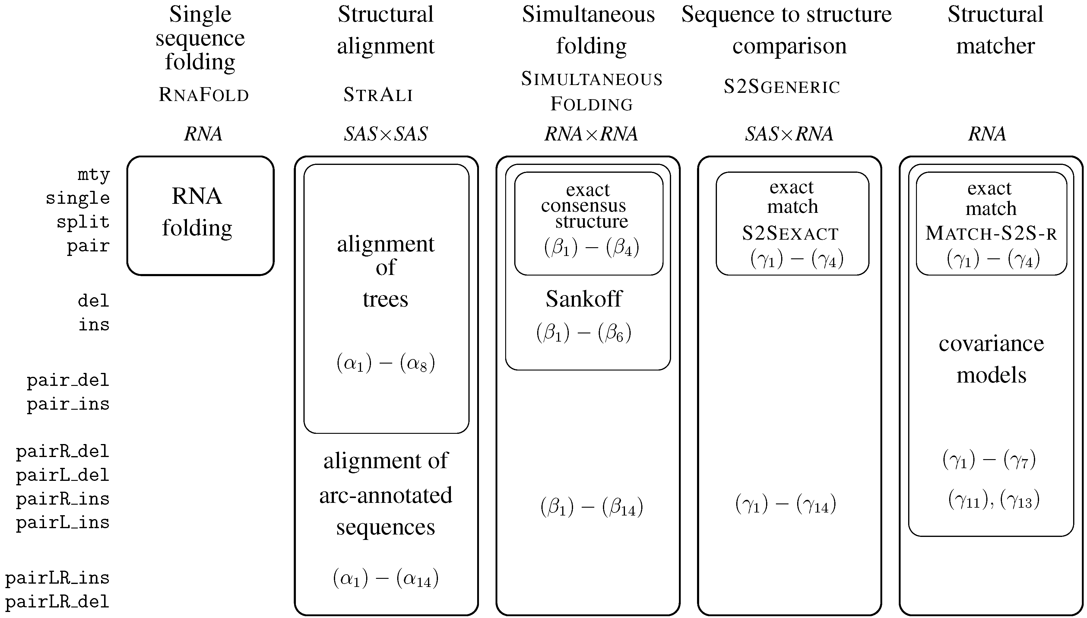
RNAfold	1	RNA folding	6.3	93
StructAli	2	struct. Alignment prototype	6.4	97
SimultaneousFolding	2	generalized fold and align	6.5	98
ExactConsensusStructure	2	exact consensus structure	6.5.2.	98
		for two RNA sequences
Sankoff	2	simultaneous fold and align	6.5.3.	99
S2SGeneric	2	covariance model, generic	6.6.1.	101
S2SExact	2	match RNA sequence	6.6.2.	100
		to target structure
Match_S2S_r	2	exact local motif matcher	6.6.4.	103
Match_S2S_r’	1	motif matcher, hard coded	6.6.4.	104
SCFG	1	stochastic context free grammar	6.3	93
CovarianceModel_r	1	covariance model, hard coded	6.6.5.	106
TreeAlign	2	classical tree alignment	7.2	111
TreeAliGeneric	2	tree alignment protoype + variants	7.2.2.	113
OsciSubforest	2	tree ali. with oscillating gaps	7.2.2.	117
TreeEdit	2	classical tree edit	7.3	119
RNATreeAli	2	RNA structure alignment	7.5	127

2. A Motivating Example

Before going to formal definitions, we start with a simple example to illustrate the main ideas behind ICOREs. We consider the classical string edit distance problem. We are given two sequences U and V, to be compared under a simple edit model. There are three edit operations: Replacement of a character symbol, deletion of a character, and insertion of a character, which can be used to transform U into V or vice versa. Each position in U and V is edited exactly once. (Without this restriction, we would arrive at the more general notion of a transformation distance. Only when the basic edit model satisfies the triangle inequality, optimal edits and transformations coincide.) The space of candidate solutions is the set of all edit scripts for U and V, defined as sequences of edit operations which transform U into V. All edit operations are associated with an additive score, and eventually, the edit script with the minimal overall score defines the edit distance between U and V.

We propose to treat these edit scripts as formal objects, and more precisely to encode them as terms. To this end, we define three function symbols, one for each edit operation: $\mathtt{rep}$, $\mathtt{del}$, and $\mathtt{ins}$. Each such operator takes as arguments the character symbol(s) involved in the operation. We also introduce a constant operator $\mathtt{mty}$, which represents the empty edit script.

For example, consider the two strings $U=$"ACGTA" and $V=$ "AATAG" on the DNA alphabet $\{\mathtt{A},\mathtt{C},\mathtt{G},\mathtt{T}\}$. One possible edit script is :

      replacement of ‘A’ by ‘A’,

      replacement of ‘C’ by ‘A’,

      deletion of        ‘G’,

      replacement of ‘T’ by ‘T’,

      replacement of ‘A’ by ‘A’,

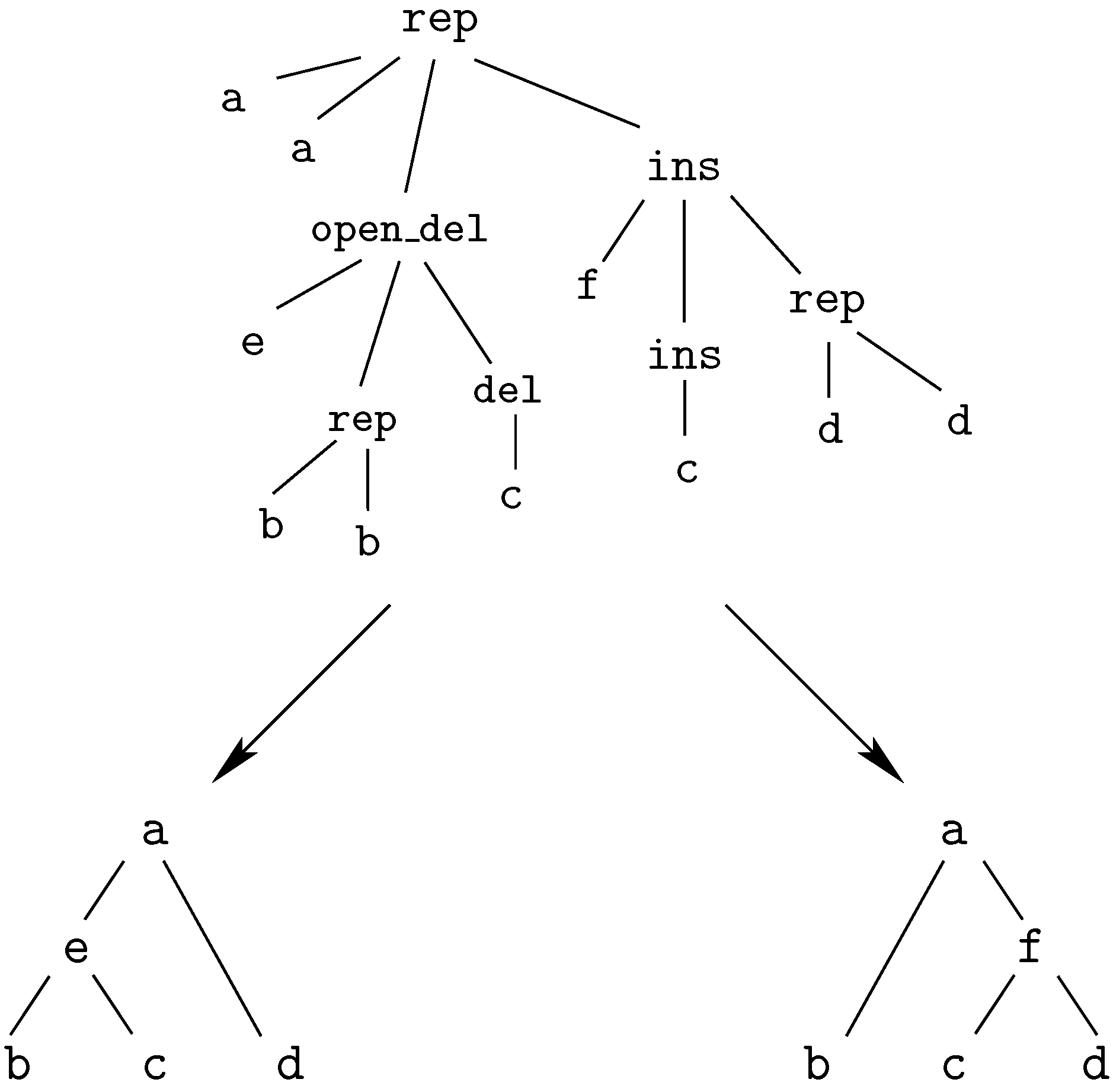
      insertion of              ‘G’

This edit script is represented by the term

          $c=$
        rep(A,A,rep(C,A,del(G,rep(T,T,rep(A,A,ins(G,mty))))))

We call these terms core terms, as they represent the search space of candidate solutions. A visually better representation of this edit script would be an alignment of the two sequences, in this case

      A C G T A -

      A A - T A G

A term representing an edit script contains in some sense the two input sequences: U is the concatenation of the first arguments of $\mathtt{rep}$ and of $\mathtt{del}$ . V is the concatenation of the second arguments of $\mathtt{rep}$ and the first arguments of $\mathtt{ins}$ . This projection is formally expressed with two term rewrite systems:

$$\begin{array}{ccccccc}\hfill \mathtt{rep}(a,b,X)& \to & a\sim X\hfill & & \hfill \mathtt{rep}(a,b,X)& \to & b\sim X\hfill \\ \hfill \mathtt{del}(a,X)& \to & a\sim X\hfill & & \hfill \mathtt{del}(a,X)& \to & X\hfill \\ \hfill \mathtt{ins}(a,X)& \to & X\hfill & & \hfill \mathtt{ins}(a,X)& \to & a\sim X\hfill \\ \hfill \mathtt{mty}& \to & \epsilon \hfill & & \hfill \mathtt{mty}& \to & \epsilon \hfill \end{array}$$

The alphabet character symbols a and b serve as nullary function symbols, extended by two operators ∼ and ε. ∼ is a binary operator for the concatenation of two strings (or a character and a string), and ε is the empty string. So U is A∼C∼G∼T∼A and V is A∼A∼T∼A∼G.

By construction, the two rewrite systems have the same left-hand sides. So we can conveniently merge their representation into a single tabular form.

$$\begin{array}{ccc}\hfill a\sim X\leftarrow & \mathtt{rep}(a,b,X)& \to b\sim X\hfill \\ \hfill a\sim X\leftarrow & \mathtt{del}(a,X)& \to X\hfill \\ \hfill X\leftarrow & \mathtt{ins}(a,X)& \to a\sim X\hfill \\ \hfill \epsilon \leftarrow & \mathtt{mty}& \to \epsilon \hfill \end{array}$$

Since we search for the optimal edit script, we need to rank all candidate terms. The operators $\{\mathtt{rep},\mathtt{del},\mathtt{ins},\mathtt{mty}\}$ constitute a signature (comparable to an interface in the programming language Java), where the operators are functions whose argument and result types are generic. Therefore, it is possible to assign a score to each core term with a score algebra implementing $\mathtt{rep}$, $\mathtt{ins}$, $\mathtt{del}$, and $\mathtt{mty}$ as functions over some concrete score data type. For example, the unit cost model used in the Levenshtein distance is expressed by the score algebra UnitScore.

$$\begin{array}{ccc}\hfill \mathtt{rep}(a,b,x)& =& ifa==b\mathrm{then}x\mathrm{else}x+1\hfill \\ \hfill \mathtt{del}(a,x)& =& x+1\hfill \\ \hfill \mathtt{ins}(a,x)& =& x+1\hfill \\ \hfill \mathtt{mty}& =& 0\hfill \\ \hfill \varphi & =& min\hfill \end{array}$$

$\varphi =min$ means that we search for the edit script of minimal cost. Under interpretation by algebra UnitScore, our example core term c evaluates to a score of 3 (which happens to be optimal).

Given these ingredients, a solution to the edit distance problem is defined as any core term which rewrites to U and V by the above rewrite rules, and evaluates under the algebra UnitScore to the optimal score of all such terms.

Signatures and terms, rewrite rules and algebras—this may seem a bit of a technical overhead for defining the Levenshtein distance of two strings. However, note that we have achieved a perfect separation of search space definition and scoring. This pays off when it comes to specifying more sophisticated problems. More flexible scoring schemes for the edit distance problem are easily provided. For example, our functions can score in a character-dependent fashion. Similarity scoring can replace distance scores, with positive scores for matches, negative scores for gaps and proper replacements, and switching to $\varphi =max$. Under a probabilistic scoring algebra, scores should multiply (rather than add up), and we better set $\mathtt{mty}=1$. Such variations to the scoring scheme only require a new algebra definition. Other changes affect the signature, and consequently the rewrite rules. We shall see in Section 5 that to introduce affine gap scoring, for example, it is enough to add operators $\mathtt{open}\_\mathtt{del}$ and $\mathtt{open}\_\mathtt{ins}$ to the signature.

In optimization there are many situations where we want to restrict the set of admissible solutions to those satisfying additional criteria. To this end, we add to our formal machinery one more feature: We will use tree grammars to restrict the universe of candidates to a subset of the algebra of core terms. Let us come back to the string edit distance problem, and specialize it at hand. We now require that an edit script must not have two adjacent indels (insertion or deletion). This type of constraint is applied, for example, in RNA-RNA interaction. We design a tree grammar that restricts the candidate space accordingly:

$$\begin{array}{ccccccccc}\hfill A^{*}& \to & \mathtt{rep}(a,b,A)\hfill & |\hfill & \mathtt{del}(a,M)\hfill & |\hfill & \mathtt{ins}(a,M)\hfill & |\hfill & \mathtt{mty}\hfill \\ \hfill M& \to & \mathtt{rep}(a,b,A)\hfill & |\hfill & \mathtt{mty}\hfill \end{array}$$

A and M are non-terminal symbols. The asterisk marks A as the axiom symbol of the grammar. The set of edit scripts satisfying the constraint on indels is exactly the language of core terms accepted by the grammar.

This concludes our informal presentation of ICOREs. The reader who feels familiar with established concepts such as signatures, rewrite rules and tree grammars may skip ahead from here to the definition of ICOREs in Section 4.

3. Machinery

We now introduce the formal definitions that will be needed throughout this article. Term rewriting is a keystone of our ICORE concept. Term rewriting is a well established computational model with a profound body of theory [17,18]. The charm of term rewrite systems as a specification formalism is that they also have a strong intuitive appeal, as everyone is used to a bit of equational reasoning from elementary algebra.

In general, term rewriting is Turing complete, and termination of term rewriting is not decidable. Here we are aiming at a certain class of combinatorial optimization problems. We will restrict term rewriting in a way such that it becomes feasible to evaluate (via dynamic programming) a search space in the following form: Given a term t, efficiently find all terms that rewrite to t, and choose from this set the best candidate under some evaluation function. Therefore, what we draw from term rewriting theory is not the full power of term rewriting, but mainly the established technical notions (i.e., signatures, rewrite relations, rewriting modulo associativity), and the fact that terms are conveniently given an algebraic interpretation. We first recall basic definitions and fix notations. Next, we introduce term rewrite systems and the restricted form in which we will use them here.

3.1. Variables, Signatures, Alphabets, Terms and Trees

We start with signatures and term algebras.

• Let $\mathcal{S}$ be a set of sorts. Sorts are names or placeholders for abstract data types.
• We assume the existence of countably infinite sets of variables $V_{\alpha }$ for every sort α of $\mathcal{S}$. The union of all $V_{\alpha }$ is denoted by V.
• We assume a finite $\mathcal{S}$-sorted signature F. An $\mathcal{S}$-sorted signature is a set of function symbols together with a sort declaration ${\alpha }_1\times \dots \times {\alpha }_n\to \alpha$ for every f of F. Here ${\alpha }_1,\cdots ,{\alpha }_n,\alpha \in \mathcal{S}$ and n is called the arity of f. Function symbols of arity 0 are called constant symbols.
• A signature F may include an alphabet $\mathcal{A}$, which is a designated subset of the nullary function symbols (constant symbols) in F. Where the distinction matters, the function symbols in $\mathcal{A}$ are called characters, and the other function symbols are called operators.
• $T(F,V)$ denotes the set of well-typed terms over F and V. It is the union of the sets $T_{\alpha }(F,V)$ for α in $\mathcal{S}$ that are inductively defined as follows:

  • each variable of $V_{\alpha }$ is a term of $T_{\alpha }(F,V)$,
  • if f is a function symbol of F with sort declaration ${\alpha }_1\times \dots \times {\alpha }_n\to \alpha$ and $t_i\in T_{{\alpha }_i}(F,V)$ for all $1\le i\le n$, then $f(t_1,\dots ,t_n)$ is in $T_{\alpha }(F,V)$.
  $T(F,V)$ is called the term algebra over F and V. The set of variables appearing in a term t is denoted by $var\left(t\right)$, and its sort by $sort\left(t\right)$ such that $sort\left(t\right)=\alpha$ when $t\in T_{\alpha }(F,V)$.
• $T\left(F\right)$ denotes the set of ground terms of $T(F,V)$, where $var\left(t\right)=\varnothing$.
• A substitution σ maps a set of variables to a set of terms, preserving sorts. The application of a substitution σ to a term t replaces all variables in t for which σ is defined by their images. The result is denoted $t\sigma$.
• Terms and trees: We adopt a dual view on terms as trees. A term can be seen as a finite rooted ordered tree, the leaves of which are labeled with constant symbols or variables. The internal nodes are labeled with function symbols of arity greater than or equal to 1, such that the outdegree of an internal node equals the arity of its label. Note that alphabet characters, being nullary function symbols, can only occur at the leaves of a tree.
• A position within a term can be represented as the sequence of positive integers that describe the path from the root to that position (the path is given in Dewey’s notation). We denote by ${t|}_p$ the subterm of t at position p and $t{\left[u\right]}_p$ the replacement of ${t|}_p$ in t by u.

3.2. Rewrite Systems

Next, we introduce term rewrite systems and the special form in which we will use them here.

• A rewrite rule is an oriented pair of terms, denoted $\ell \to r$, such that $sort\left(\ell \right)=sort\left(r\right)$ and $var\left(r\right)\subseteq var\left(\ell \right)$. Because of the last requirement, generally $r\to \ell$ is not a legal rewrite rule, and rewrite rules cannot be reversed without generating unbound variables. Furthermore, we disallow $\ell \in V$, as such a rule would allow to rewrite any term, while $r\in V$ is perfectly legal.
• A term rewrite system R is a finite set of such rewrite rules. The rewrite relation induced by R, written ${\to }_R$, is the smallest relation closed under context and substitution containing each rule of R. In other words, a term t rewrites to a term u, written $t{\to }_{R}u$, if there exist a position p in t, a rule $\ell \to r$ in R and a substitution σ such that ${t|}_p=\ell \sigma$ and $u=t{\left[r\sigma \right]}_p$. ${\to }_R^{*}$ is the reflexive transitive closure of ${\to }_R$.
• In the sequel, we will consider term rewrite systems with disjoint signatures. We say that R is a term rewrite system with disjoint signatures if it is possible to partition F into two subsets ζ and Σ such that for each rule $\ell \to r$ of R, the left-hand side ℓ belongs to $T(\zeta ,V)$, and the right-hand side r belongs to $T(\Sigma ,V)$. In this manuscript, ζ is called the core signature, and Σ the satellite signature. Ground terms of $T\left(\zeta \right)$ are called core terms. ζ and Σ can both contain an associative binary operator, denoted ${\sim }_{\zeta }$ and ${\sim }_{\Sigma }$ respectively (see below).
  In practice, core signatures may share function symbols with satellite signatures (possibly not with the same arity). Often, they share the alphabet. By convention, when a shared symbol occurs in a rewrite rule, it belongs to the signature ζ on the left-hand side, and to Σ on the right-hand side. Elsewhere, symbols of ζ will be subscripted for clarity.
• Syntactic conditions: Rewrite rules may have associated syntactic conditions for their applicability, as in

  $$f(a,b,X)\to X\sim a\mathbf{if}a=b\mathrm{for}a,b\in \mathcal{A}$$
  In our framework, these conditions will only refer to characters from a finite alphabet. This is merely a shorthand against having to write too many similar rules, and does not contribute computational power. It must not be confused with general conditional term rewriting as in $f(x,y)+y\to 2*x\mathbf{if}x=y$, where the rule is applicable if x and y can be rewritten to a joint reduct by the given rewrite system.

3.3. Rewriting Modulo Associativity

In certain applications, we will use rewriting modulo associativity. In such cases, the signature contains an associative binary function symbol, always denoted ∼. For each such symbol ∼, we provide a neutral element symbol ε and a set of equations, which are to be seen as symmetric rules:

$$\begin{array}{ccccc}\hfill A& =& \{\hfill & (X\sim Y)\sim Z=X\sim (Y\sim Z),X\sim \epsilon =X,\epsilon \sim X=X\hfill & \}\hfill \end{array}$$

${=}_A$ is the smallest equivalence relation closed under context and substitution containing A. A term t rewrites modulo A to a term u for the rewrite rule $\ell \to r$, denoted $t{\to }_{A,\ell \to r}u$ if there exist two terms $t^{\prime }$ and $u^{\prime }$ such that $t{=}_A{t}^{\prime }$, $u{=}_A{u}^{\prime }$ and $t^{\prime }$ rewrites to $u^{\prime }$ by the rule $\ell \to r$.

Why do we need such associative function symbols? The first reason is that strings can be described alternatively as compositions of unary functions or as sequences of nullary operator symbols. The first case appears somewhat artificial. In the latter case, we need to introduce one extra, binary associative operator ∼. Consider nullary function symbols a, b, c and d, the term a∼b∼c∼d refers to the string "abcd". This notation is convenient to do pattern matching on sequence input. For example, the term X∼a∼b∼Y will match to any occurence of "ab" in a longer sequence, and X∼a∼b∼Y∼a∼b∼Z to any repeated occurence, with interspersed characters matched to Y. Where used, associativity adds quite a bit of expressiveness to rewrite systems.

Aside from convenience when dealing with strings, the second reason to use the operator ∼ comes from the desire to include problems defined on ordered, labeled, rooted trees in our framework. They are commonly not defined over a signature, but over an (untyped) operator alphabet where each operator can label any tree node with any number of subtrees. Considering them as function symbols, they have flexible arity, and use only a single sort. A “tree node labeled f” with a variable number of subtrees, such as $f(x,y)$ and $f(x,y,z)$, will be written in our framework as $f(x\sim y)$ and $f(x\sim y\sim z)$, which allows us to specify f as a unary operator in the signature.

3.4. Tree Grammars

A signature F defines a language of terms, $T\left(F\right)$. We will provide the possibility to limit the set of terms under consideration by the use of tree grammars. ( Our dual view on terms as trees is not strictly necessary. Our tree grammars are actually “term grammars”, describing subsets of $T\left(F\right)$. Our tree alignments, discussed later, could as well be called “term alignments”, and so on. However, when terms are considered as data structures, as we do it here, the tree terminology is the more established one.) A tree grammar $\mathcal{G}$ over a signature F is defined by the tuple $\mathcal{G}=(N,F,Z,P)$, where

• F is the signature,
• N is a set of non-terminal symbols, disjoint from F, where each element is assigned a sort.
• Z is the starting non-terminal symbol, with $Z\in N$, and
• P is a set of productions of the form $X\to t$, where $X\in N$, $t\in T(F,N)$, and X and t have the same sort.

$L\left(\mathcal{G}\right)$ denotes the language of $\mathcal{G}$. It is the (sub)set of terms of $T\left(F\right)$ that can be derived from Z using productions of P.

3.5. Algebras

Every aspect of scoring and applying objective functions in our combinatorial optimization problems will be modeled by algebras.

• Given signature F, an F-algebra A associates a carrier set (i.e., a concrete data type) with each sort symbol in F, and a function of the corresponding type with each $f\in F$. $A\left(t\right)$ denotes the value obtained by evaluating term t under the interpretation given by algebra A. Often, we shall provide several algebras to evaluate terms.
• An objective function is a function ϕ$:M\to M$, where M is the domain of multisets (bags) over some carrier set in a given algebra. (Multiple carrier sets give rise to one overloaded instance of ϕ on each carrier set.) Typically, ϕ will be minimization or maximization, but summation, enumeration, or sampling are also common. Our objective functions are defined on multisets rather than sets, as we want to model problems such as finding all co-optimal solutions of a problem instance.
• An F-algebra augmented by an objective function for multisets over each of its carrier sets is called an evaluation algebra.

Up to here, we have collected technical notions that have been used in diverse fields of theoretical computer science. We are now going to assemble them to make ICOREs.

4. Inverse Coupled Rewrite Systems

In this section, we make concrete the sketch of ideas laid out in Section 2. We give the formal definition of ICORES and their semantics, and suggest a semi-formal notation in which examples will be presented.

4.1. ICORE Definitions

Definition 1.

Inverse coupled rewrite system.

Let k be a positive natural number. An ICORE of dimension k consists of

• a set V of variables,
• a core signature ζ, and k satellite signatures ${\Sigma }_1,\cdots ,{\Sigma }_k$, such that $\zeta \cap ({\Sigma }_1\cup \dots \cup {\Sigma }_k)=\varnothing$. (Function symbols of ζ are disjoint from all ${\Sigma }_i$, except for a possible shared alphabet.)
• k term rewrite systems with disjoint signatures, $R_1,\dots ,R_k$, which all have the same left-hand sides in $T(\zeta ,V)$. (Those systems are called the satellite rewrite systems.)
• optionally a tree grammar $\mathcal{G}$ over the core signature ζ,
• an evaluation algebra A for the core signature ζ, including an objective function ϕ.

□

In the satellite rewrite systems, the multiple right-hand sides for the same left-hand side are also called rule projections and are written in the form $r_1\leftarrow \ell \to r_2$ for $k=2$, or with a double arrow $\ell \Rightarrow r_1|\cdots |r_k$ for any dimension k.

Since the core signature and the satellite signatures are disjoint, each rewrite step erases all operator symbols present in the left-hand side of the rewrite rules, and all satellite rewrite systems are terminating. No part of a term can be rewritten twice: Once an function symbol is read as part of a left-hand side, it is consumed. This ensures that a position in a term may take part in a rewrite only once, which corresponds to the classical edit model in string comparison: Each character in a string is to be edited at most once. This essential restriction compared to general term rewriting will be further discussed in Section 9.4.

How to compute with an ICORE? We introduce the notion of coupled rewriting which means in simple words that a core term is rewritten into k satellite terms by using the same rewrite rules in the same positions. Technically, this definition is a bit complicated as it requires to keep track of what are “same” positions over a series of rewrite steps.

Definition 2.

Coupled rewrite relation. Let c be a core term of $T(\zeta ,V)$, seen as a tree (This means that ∼ symbols are omitted, and the position of a symbol is not modified when we apply associativity of ∼). We provide each operator symbol occuring in c with its initial position in c (for example using Dewey’s notation). A coupled rewrite of c is a sequence of k rewrite derivations $c{\to }_{R_1}^{*}{t}_1$, ..., $c{\to }_{R_k}^{*}{t}_k$ such that there exist some number j and intermediate reducts $(t_1^0,\dots ,t_1^j),\dots ,(t_k^0,\dots ,t_k^j)$ satisfying

• $c=t_1^0=\cdots =t_k^0$ (start of a coupled derivation),
• $t_1=t_1^j$, ..., $t_k=t_k^j$ (end of a coupled derivation),
• for each e, $0\le e<j$ (step in a coupled derivation), there exists a rule projection $\ell \Rightarrow r_1|\cdots |r_k$ such that $t_i^e$ rewrites modulo associativity to $t_i^{e+1}$ with the rule $\ell \to r_i$ and all rewrites apply simultaneously at the same place. In other words, for each i, there is a term $v_i$, a position $p_i$ in $v_i$ and a substitution ${\sigma }_i$ such that $t_i^e{=}_A{v}_i$, $v_i{|}_{p_i}=\ell {\sigma }_i$, $t_i^{e+1}=v_i{\left[r{\sigma }_i\right]}_{p_i}$, and all operator symbols in ℓ have the same initial position in c.

□

In the sequel, we shall write $t_1{\leftarrow }^{*}c{\to }^{*}{t}_2$ to denote that $c{\to }^{*}{t}_1$ and $c{\to }^{*}{t}_2$ is a coupled derivation. We will use the double arrow symbol to designate a coupled rewrite of a core term c for any dimension k, $c{\Rightarrow }^{*}{t}_1|\cdots |t_k$ .

Example 1. In Section 2, we have introduced an ICORE of dimension 2 for the string edit distance problem with core signature operators $\{\mathtt{rep},\mathtt{ins},\mathtt{del},\mathtt{mty}\}$. For this ICORE, the core term $c=\mathtt{rep}(\mathtt{A},\mathtt{A},\mathtt{rep}(\mathtt{C},\mathtt{A},\mathtt{del}(\mathtt{G},\mathtt{rep}(\mathtt{T},\mathtt{T},\mathtt{rep}(\mathtt{A},\mathtt{A},\mathtt{ins}(\mathtt{G},\mathtt{mty}\left)\right)\left)\right)\left)\right)$ allows for the following coupled rewriting derivation.

$$\begin{array}{cc}\multicolumn{2}{c}{\underline{\mathtt{rep}}(\mathtt{A},\mathtt{A},\mathtt{rep}(\mathtt{C},\mathtt{A},\mathtt{del}(\mathtt{G},\mathtt{rep}(\mathtt{T},\mathtt{T},\mathtt{rep}(\mathtt{A},\mathtt{A},\mathtt{ins}(\mathtt{G},\mathtt{mty}))))))}\\ \swarrow & \searrow \\ \mathtt{A}\sim \underline{\mathtt{rep}}(\mathtt{C},\mathtt{A},\mathtt{del}(\mathtt{G},\mathtt{rep}(\mathtt{T},\mathtt{T},\mathtt{rep}(\mathtt{A},\mathtt{A},\mathtt{ins}(\mathtt{G},\mathtt{mty})))))& \mathtt{A}\sim \underline{\mathtt{rep}}(\mathtt{C},\mathtt{A},\mathtt{del}(\mathtt{G},\mathtt{rep}(\mathtt{T},\mathtt{T},\mathtt{rep}(\mathtt{A},\mathtt{A},\mathtt{ins}(\mathtt{G},\mathtt{mty})))))\\ \downarrow & \downarrow \\ \mathtt{A}\sim \mathtt{C}\sim \underline{\mathtt{del}}(\mathtt{G},\mathtt{rep}(\mathtt{T},\mathtt{T},\mathtt{rep}(\mathtt{A},\mathtt{A},\mathtt{ins}(\mathtt{G},\mathtt{mty}))))& \mathtt{A}\sim \mathtt{A}\sim \underline{\mathtt{del}}(\mathtt{G},\mathtt{rep}(\mathtt{T},\mathtt{T},\mathtt{rep}(\mathtt{A},\mathtt{A},\mathtt{ins}(\mathtt{G},\mathtt{mty}))))\\ \downarrow & \downarrow \\ \mathtt{A}\sim \mathtt{C}\sim \mathtt{G}\sim \underline{\mathtt{rep}}(\mathtt{T},\mathtt{T},\mathtt{rep}(\mathtt{A},\mathtt{A},\mathtt{ins}(\mathtt{G},\mathtt{mty})))& \mathtt{A}\sim \mathtt{A}\sim \underline{\mathtt{rep}}(\mathtt{T},\mathtt{T},\mathtt{rep}(\mathtt{A},\mathtt{A},\mathtt{ins}(\mathtt{G},\mathtt{mty})))\\ \downarrow & \downarrow \\ \mathtt{A}\sim \mathtt{C}\sim \mathtt{G}\sim \mathtt{T}\sim \underline{\mathtt{rep}}(\mathtt{A},\mathtt{A},\mathtt{ins}(\mathtt{G},\mathtt{mty}))& \mathtt{A}\sim \mathtt{A}\sim \mathtt{T}\sim \underline{\mathtt{rep}}(\mathtt{A},\mathtt{A},\mathtt{ins}(\mathtt{G},\mathtt{mty}))\\ \downarrow & \downarrow \\ \mathtt{A}\sim \mathtt{C}\sim \mathtt{G}\sim \mathtt{T}\sim \mathtt{A}\sim \underline{\mathtt{ins}}(\mathtt{G},\mathtt{mty})& \mathtt{A}\sim \mathtt{A}\sim \mathtt{T}\sim \mathtt{A}\sim \underline{\mathtt{ins}}(\mathtt{G},\mathtt{mty})\\ \downarrow & \downarrow \\ \mathtt{A}\sim \mathtt{C}\sim \mathtt{G}\sim \mathtt{T}\sim \mathtt{A}\sim \underline{\mathtt{mty}}& \mathtt{A}\sim \mathtt{A}\sim \mathtt{T}\sim \mathtt{A}\sim \mathtt{G}\sim \underline{\mathtt{mty}}\\ \downarrow & \downarrow \\ \mathtt{A}\sim \mathtt{C}\sim \mathtt{G}\sim \mathtt{T}\sim \mathtt{A}& \mathtt{A}\sim \mathtt{A}\sim \mathtt{T}\sim \mathtt{A}\sim \mathtt{G}\end{array}$$

At each step, the active function symbol involved in the rewriting is underlined. We say that the two strings "ACGTA" and "AATAG" are the coupled reducts of c, or equivalently that c is an inverse coupled reduct of "ACGTA" and "AATAG" . We write

$$“\mathtt{ACGTA}”{\leftarrow }^{*}t{\to }^{*}“\mathtt{AATAG}”$$

□

In the above example, aside from the core term c, there are many other core terms that also rewrite to the two satellite inputs. Together, they constitute the search space of an optimization problem.

Definition 3. ICORE candidate solutions. Given a k-tuple of satellite terms $(t_1,\dots ,t_k)$, the set of candidate solutions for $(t_1,\dots ,t_k)$ is the set of core terms c such that

• c is recognized by the tree grammar: $c\in L\left(\mathcal{G}\right)$, and
• c has a coupled rewriting into all inputs: $c{\Rightarrow }^{*}{t}_1\left|\dots \right|t_k$.

□

Fact 1. The set of candidate solutions of an ICORE is recursive.

Proof. This comes from the fact that each rewrite system in an ICORE is terminating. Hence, there is only a finite number of derivations starting from a given core term, and all these derivations are finite.  □

We do not go into deeper details about efficient algorithms to build the set of candidate solutions. This is out of the scope of this paper. Some lines of research will be exposed in Section 10. Which problem an ICORE actually solves is given by the set of optimal candidate solutions. This set depends on the evaluation algebra and its objective function.

Definition 4. Solution of an ICORE. Given an ICORE and a k-tuple $(t_1,\dots ,t_k)$ in $T\left({\Sigma }_1\right)\times \cdots \times T\left({\Sigma }_k\right)$, the multiset of optimal solutions is given by

$$\varphi \left(\right[A\left(c\right)|c\in L\left(\mathcal{G}\right),c{\Rightarrow }^{*}{t}_1\left|\dots \right|t_k\left]\right)$$

□

The use of multisets in this definition calls for some explanation. Although the most common application in our type of problem is to compute a single answer, we also want to do k-best optimization, or return all answers up to a score threshold. There is no upper limit on the number of answers, which calls for a answer set. Furthermore, there may be cases (some times for certain sub-problems) where no solution exists, which is gracefully handled by returning ∅. But why multi-sets? While $c\in L\left(\mathcal{G}\right)$ denotes a set, $\left[A\right(c\left)\right|c\in L\left(\mathcal{G}\right),\dots ]$ denotes a multiset, because several candidates may evaluate to the same score under A. We want to be able to speak, for example, about the number of co-optimal candidates in a solution. These candidates may be evaluated under a second algebra B and selected from by yet another choice function associated with B. Of all the most tasty pizzas in our search space, we want the cheapest ...–more on this in Section 8. This is why we provide for multiple elements in Definition 4.

Definition 4 makes clear why we speak of inverse rewrite systems. While c rewrites to $t_1,\dots ,t_k$ by the rules of $R_1,\dots ,R_k$, terms $t_i$ are the actual inputs of a problem instance, and the core term c must be found by constructing in reverse the (coupled) rewrites $c{\to }^{*}{t}_i$, for all such c.

Definitions 1, 2, 3 and 4 complete our formal framework of ICOREs. Later, in Section 8, we will introduce operations that built sophisticated evaluation algebras from simpler ones. Since such a product of two algebras is just another algebra, this will add convenience, but not a conceptual extension to ICOREs.

4.2. ICORE Pseudocode

Let us introduce a semi-formal, pseudocode notation for ICOREs. Our goal is to describe ICOREs in a way that is both concise–easy to write and read–and complete in the sense that there is all information required to actually compile the ICORE into executable code. And even more: we want a certain level of redundancy that allows a compiler to safeguard against human errors. For example, types of functions must be declared, although in principle, it might be possible to infer them automatically. The notation we propose here is preliminary and open to change.

ICORE presentation. We summarize our string edit distance example of Section 2 in ICORE EditDistance in our pseudocode. We assume the alphabet $\mathcal{A}$ to be known from the context, but it could also be listed explicitly or be declared as one of a set of predefined alphabets, such as all ASCII characters or the DNA alphabet $\{\mathtt{A},\mathtt{C},\mathtt{G},\mathtt{T}\}$.

The first line gives the name of the ICORE and its dimension, i.e. the number of inputs. The first satellite signature is explicitly declared, while its name $SEQ$ is simply re-used for the second satellite signature. Two dashes start a comment that extends until the end of the line. Specifying $T\left(ALI\right)$ in place of a tree grammar, we express that all core terms are legal members of the overall search space. (Although not needed here, we strongly recommend the use of tree grammars to explicitly restrict the search space. This is safer than the common practice of making such restrictions the responsibility of the scoring scheme, for example by penalizing mal-formed candidates with a score of $\pm \infty$. In that case, we still have an unknown number of zombies that populate the search space. They may not surface as optimal solutions, but how about evaluating, in addition, the size of the search space, or compute a score average ...?]) The rewrite rule set is not given an extra name, but is refered to by the ICORE name if necessary.

An arbitrary number of algebras for the core signature can be specified. Here we only show algebra UnitScore. Next to the algebra name, the carrier sets for all the sorts in the signature are specified. Here, there is only one sort, $Ali$, which is interpreted by natural numbers. Functions operating on such values, such as min and +, are imported from a suitable programming environment.

For functional programmers, a signature such as $ALI$ resembles an algebraic data type, here with constructors $\{\mathtt{rep},\mathtt{del},\mathtt{ins},\mathtt{mty}\}$. In fact, such a data type can be supplied as an algebra for enumerating the search space in symbolic form. While infeasible for realistic input sizes, it is instructive to do such enumeration on small inputs during program development.

We will always present the components of an ICORE in the above order, although there is no intrinsic need for it. As these concepts are declarative, any order would have the same meaning, as given by Definition 4. We give explicit names to many ICORE components, and allow them to be imported by name and possibly extended in further ICOREs. We will make extensive use of inheritance (as in object oriented languages) by means of an extends … with … construct.

Further notational conventions. As we deal with a large number of ICORE examples, introducing an even larger number of component names, we adhere to the following naming conventions.

• ICORE, grammar and algebra names are written in small Capitals.
• Signatures have three- or four-letter names in ITA LICS.
• Sort names have an inital upper-case letter.
• Operators are written in typewriter font.
• Concrete alphabet symbols are written in typewriter font, such as A, +.
• Variables $a,b,c$ refer to alphabet characters, $X,Y,Z$ to (sub-)terms in rewrite rules (that may undergo further rewriting), and $x,y,z$ to values derived from core terms in some algebra.
• The variable w is reserved for multisets of candidate values, on which objective functions operate.

4.3. An ICORE Exercise

Although our ICORE notation as introduced above requires quite some detail, ICORE design starts on a more informal level. In this section, we define a small but non-trivial problem to be solved, sketch the first design ideas, and leave it to the reader to add in the remaining detail. Our problem is the following: Given two strings, we want to determine their minimal Hamming distance under the unusual convention that palindromic subsequences in either input string may be ignored, contributing a fixed score of 1 (independent of their length) to the distance. This turns the Hamming distance problem into an optimization problem, because different decisions about which palindromes to ignore lead to different scores.

Example 2. For the sequences "aabbccbb" and "aaccbbaa", we have distance scores of 2, 3, 4, and 6 for four example candidates:

    

aaBBccbb          aa  bBCCBb       AABBccbb       aabbccbb

    

aa  ccbbAA        aaCCb    bAA     AA  ccbbAA     aaccbbaa

where the capital letters indicate the palindrome choices, and the small letters the matched characters. Note that "AABB" marks two adjacent palindromes of length 2 in the third case. Of course, there are many more candidates which must be considered to find the minimum.  □

As the input data types are normally clear when a problem is posed, the first step in ICORE design is to decide upon the signature of core terms ( In a sense, this overthrows common practice and most textbook advice on dynamic programming (unless you already adhere to the algebraic style). There, a data type representing candidate solutions is not defined explicitly. In the implementation, we clearly do not want to explicitly represent a search space of exponential size. But for developing an algorithm, the candidate trees are really at the heart of the design. We trust on our eventual ICORE compiler to perform the deforestation, taking care that candidates are evaluated instead of explicitly constructed. We will return to this aspect in the concluding discussion.) All the situations that we want to distinguish and score differently must be captured, so it is good to draw an example candidate as a tree. The leftmost candidate of the above might look like this:

This example hopefully contains all the relevant cases. Note that with $\mathtt{rep}$, only one character is specified. In this application, “replacements” are exact matches, and there is no need to have the same character twice in the core term. Distinguishing matched parts from ignored palindromes calls for a signature with two sorts: A for any kind of sequences and P for palindromic sequences.

Core signature

$$\begin{array}{ccccc}\mathtt{rep}& \hfill :& \hfill A\times S& \to & S\hfill \\ \mathtt{mty}& \hfill :& & & S\hfill \\ \mathtt{dpal}& \hfill :& \hfill P\times S& \to & S\hfill \\ \mathtt{ipal}& \hfill :& \hfill S\times P& \to & S\hfill \\ \mathtt{pal}& \hfill :& \hfill A\times P& \to & P\hfill \\ \mathtt{turn}& \hfill :& & \to & P\hfill \end{array}$$

$\mathtt{dpal}$ is used to initiate a palindrome in the first input, $\mathtt{ipal}$ one in the second input. Even if we plan to score these cases symmetrically, we must distinguish them, because they must rewrite differently. $\mathtt{pal}$ generates the palindrome characters; each character is represented just once. Now let us try for some rewrite rules. The first two deal with character matches, the others deal with palindromes:

$$\begin{array}{ccc}\hfill a\sim S\leftarrow & \mathtt{rep}(a,S)& \to a\sim S\hfill \\ \hfill \epsilon \leftarrow & \mathtt{mty}& \to \epsilon \hfill \\ \hfill P\sim S\leftarrow & \mathtt{dpal}(P,S)& \to S\hfill \\ \hfill S\leftarrow & \mathtt{ipal}(S,P)& \to P\sim S\hfill \\ \hfill a\sim P\sim a\leftarrow & \mathtt{pal}(a,P)& \to a\sim P\sim a\hfill \\ \hfill \epsilon \leftarrow & \mathtt{turn}& \to \epsilon \hfill \end{array}$$

With these rules, our candidate term must have a coupled rewrite to the inputs. It is insightful to perform the coupled rewrite by hand a few times. For

$$t=\mathtt{rep}(\mathtt{a},\mathtt{rep}(\mathtt{a},\mathtt{dpal}(\mathtt{pal}(\mathtt{b},\mathtt{turn}),\mathtt{rep}(\mathtt{c},t^{\prime }))))\mathrm{where}$$

$$t^{\prime }=\mathtt{rep}(\mathtt{c},\mathtt{rep}(\mathtt{b},\mathtt{rep}(\mathtt{b},\mathtt{ipal}(\mathtt{mty},\mathtt{pal}(\mathtt{a},\mathtt{turn})))))$$

we find

$$“\mathtt{aabbccbb}”\leftarrow t\to “\mathtt{aaccbbaa}”$$

as expected. Thus, our design might be on the right track. We leave it to the reader to try write down the other candidates as terms, and to add some scoring algebras. The first would be an algebra B such that $B\left(t\right)=2$ as postulated above. Which operator(s) should account for the palindrome score? Should we worry about empty palindromes? Have we covered single-letter and odd-length palindromes at all? What if we wanted to assign, more generally than formulated above, an affine, length dependent score to palindromes? And so on. Have fun.

4.4. Why Rewriting the Wrong Way?

Before we proceed to real-world applications, let us reflect for a moment on the “inverse” in ICOREs. Why do we specify problems by rewriting solutions to inputs, rather than the other way round?

Satellites terms pose problem instances and define a search space of different solutions. Core terms represent individual solutions, and all details of scoring. In doing so, core terms are more concrete than satellites. Mapping from concrete to abstract is always the simpler direction–all the information is there, we just transform it and may discard parts of it. Left-hand sides match the core term, right-hand sides produce the satellite. Variables on the left-hand side are instantiated to parts of the the core term, but may be dropped in the emerging satellite. Good for us, as this makes our rewrite rules well-formed, satisfying the requirement $var\left(r\right)\subset var\left(l\right)$. Trying to rewrite the other way, from abstract to concrete, detail must be generated, and unless the solution is unique, it must be chosen from many possibilities by an optimization process. Technically, the reversed rewrite rules would introduce free variables, to be instantiated by a search process. This process must be described, for example, by crafting DP recurrences, and we are back at the cumbersome and low-level practices of the past.

The convenience offered by ICOREs come from the fact that we allow designers to specify their problem in the easy direction: CONCRETE → ABSTRACT, or RESULT → PROBLEM, and the semantics of ICOREs reverses the direction. Definition 4 requires to construct the whole search space and evaluate it efficiently. In simple words: Modelers describe how answers relate to questions, and we hope to automatically provide the transformation from questions to answers.

5. ICOREs for Sequence Analysis

We have used the string edit distance as an expository example in Section 2. We now demonstrate the expressivity and the universality of the ICORE framework on several other popular problems in sequence analysis. Sequence comparison is used in many flavours in computational biology, dealing with DNA, RNA or protein sequences. Just as well, we might be comparing text documents or sequences of peaks from mass spectrum analysis. We will consider alignments with affine gap models, local search, and approximate matching, and show how ICOREs allow to move from a given problem to another one in a systematic way. Figure 1 summarizes all these problems. Throughout this section, we assume a generic alphabet $\mathcal{A}$ and use the core signature $ALI=\mathcal{A}\cup \{\mathtt{mty},\mathtt{rep},\mathtt{ins},\mathtt{del}\}$.

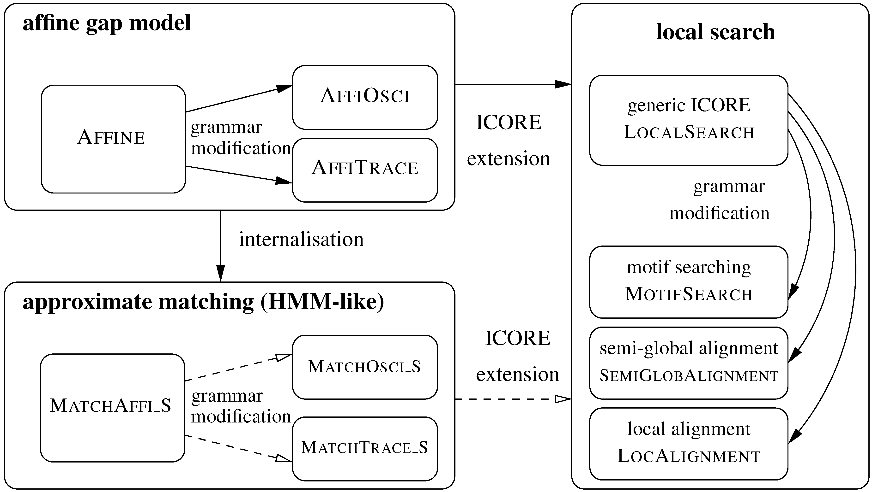
5.1. Sequence Comparison with an Affine Gap Model

5.1.1. Standard Affine Gap Model

We refine the simple edit distance approach with an affine gap model, such as introduced in Gotoh’s algorithm [19]. The idea of affine gap scoring is that a gap of length n should be charged a cost of type $o+(n-1)e$, where o is a (high) initial “opening” charge while e is a smaller charge for gap extension. This model is motivated, for example, by gene comparison, where breakage of the DNA is rare, but once it is broken, an insertion or deletion of any length is likely. For that, we need to introduce new operators in the core signature, $\mathtt{open}\_\mathtt{del}$ and $\mathtt{open}\_\mathtt{ins}$, while we retain $\mathtt{del}$ and $\mathtt{ins}$ which now designate gap extension.

Figure 1. Overview of sequence analysis problems addressed in Section 5. Solid arrow lines indicate transformations between icores that are detailed in the text. Dashed arrow lines indicate transformations that are left as exercise for the reader.

Figure 1. Overview of sequence analysis problems addressed in Section 5. Solid arrow lines indicate transformations between icores that are detailed in the text. Dashed arrow lines indicate transformations that are left as exercise for the reader.

ICORE Affine is our first case where it is convenient to use a tree grammar for defining precisely the candidate space. The grammar ensures that each gap begins indeed with a gap opening, followed possibly by extension operations. One can note that the dependency graph (Recall the definition of a dependency graph of a grammar: the nodes are the non-terminal symbols. There is an edge from the node labeled by the non-terminal S to the node labeled by the non-terminal T if there is a production of the form $S\to c\left(T\right)$) of the grammar Affi has the same architecture as the finite state transducer usually associated to alignments with affine gap costs, such as displayed in a classical textbook ([20], chapter 2). This transducer takes as input the first string, and outputs the second string. The edit script is obtained as the list of states visited, and each transition arc can be assigned a score. Figure 2a shows this transducer, and 2b shows the dependency graph of Affi.

Figure 2. (a) Finite State Automaton for alignment with affine gap weights (source [20]); (b) Dependency graph for the grammar Affi; (c) for the grammar AffiOsci; (d) and for the grammar AffiTrace. The start state/axiom symbol is marked by an arrowhead.

Figure 2. (a) Finite State Automaton for alignment with affine gap weights (source [20]); (b) Dependency graph for the grammar Affi; (c) for the grammar AffiOsci; (d) and for the grammar AffiTrace. The start state/axiom symbol is marked by an arrowhead.

Example 3. For the pair of sequences "GCTGTCCA" and "ACGAATGCA" the core term

$$\begin{array}{c}c=\mathtt{rep}(\mathtt{G},\mathtt{A},\mathtt{rep}(\mathtt{C},\mathtt{C},\mathtt{open}\_\mathtt{ins}(G,\mathtt{ins}(\mathtt{A},\mathtt{ins}(\mathtt{A},\mathtt{rep}(\mathtt{T},\mathtt{T},\mathtt{rep}(\mathtt{G},\mathtt{G},\\ \mathtt{open}\_\mathtt{del}(\mathtt{T},\mathtt{del}(\mathtt{C},\mathtt{rep}(\mathtt{C},\mathtt{C},\mathtt{rep}(\mathtt{A},\mathtt{A},\mathtt{mty}\left)\right)\left)\right)\left)\right)\left)\right)\left)\right))\end{array}$$

encodes the alignment

      G C - - - T G T C C A

        |       | |     | |

      A C G A A T G - - C A

On the other side, a term such as $\mathtt{rep}(\mathtt{A},\mathtt{A},\mathtt{del}(\mathtt{T},\mathtt{rep}(\mathtt{G},\mathtt{T},\mathtt{mty})\left)\right)$ is banned by the grammar because the gap extension has no preceding gap opening. It does not correspond to a legal alignment in the affine gap model. A borderline example is a term such as $\mathtt{rep}(\mathtt{A},\mathtt{C},\mathtt{open}\_del(\mathtt{G},\mathtt{del}(\mathtt{A},\mathtt{open}\_\mathtt{del}(\mathtt{T},\mathtt{mty}\left)\right)\left)\right)$ , because the “same” gap contains two gap opening operations. Many formulations of affine gap alignment allow for this case–it will never score optimally, so why care. However, should we be interested also in near-optimal solutions, it is more systematic to keep malformed candidates out of the search space. Our grammar rules out this candidate solution.  □

5.1.2. Variants of the Affine Gap Model: Oscillating Gaps and Traces

By modifying the grammar Affi, we can also adjust the kinds of alignments actually considered in search of the optimal one. We give two such examples.

In a first variant, let us provide for oscillating gaps. With grammar Affi, adjacent deletions/insertions or vice versa are charged two gap opening costs. With oscillating gaps, switching from a deletion directly to an insertion (or from an insertion directly to an insertion) is not charged by an extra gap opening cost. To express this change, we merely have to replace the grammar Affi with AffiOsci. Rather than two distinct gap modes–nonterminal symbols D and I, we only have a single state G. (Experts know that in the implementation, this reduces three dynamic programming tables to two.) The dependency graph is given in Figure 2c.

Grammar Affiosci

$$\begin{array}{ccccccccc}\hfill A& \to & \mathtt{rep}(a,b,A)\hfill & |\hfill & \mathtt{open}\_\mathtt{del}(a,G)\hfill & |\hfill & \mathtt{open}\_\mathtt{ins}(a,G)\hfill & |\hfill & \mathtt{mty}\hfill \\ \hfill G& \to & \mathtt{del}(a,G)\hfill & |\hfill & \mathtt{ins}(a,G)\hfill & |\hfill & \mathtt{rep}(a,b,A)\hfill & |\hfill & \mathtt{mty}\hfill \end{array}$$

In the second variant, we consider traces rather than alignments. The trace of an alignment is the sequence of matched residues. This means that traces do not specify an order between adjacent deletions and insertions. In the graphical representation of an alignment, this can be modeled by enforcing a convention that deletions always precede adjacent insertions. In the following example, the leftmost alignment satisfies the trace condition, the others are considered redundant.

    AACC--TT    AA--CCTT    AA-CC-TT   AAC-C-TT    AAC--CTT

    ||    ||    ||    ||    ||    ||   ||    ||    ||    ||

    AA--GGTT    AAGG--TT    AAG--GTT   AA-G-GTT    AA-GG-TT

Starting from grammar Affi, we design grammar AffiTrace, which disallows transitions from state I into state D. The dependency graph is given in Figure 2d.

Grammar AffiTrace

$$\begin{array}{ccccccccc}\hfill A& \to & \mathtt{rep}(a,b,A)\hfill & |\hfill & \mathtt{open}\_\mathtt{del}(a,D)\hfill & |\hfill & \mathtt{open}\_\mathtt{ins}(a,I)\hfill & |\hfill & \mathtt{mty}\hfill \\ \hfill D& \to & \mathtt{del}(a,D)\hfill & |\hfill & \mathtt{rep}(a,b,A)\hfill & |\hfill & \mathtt{open}\_\mathtt{ins}(a,I)\hfill & |\hfill & \mathtt{mty}\hfill \\ \hfill I& \to & \mathtt{ins}(a,I)\hfill & |\hfill & \mathtt{rep}(a,b,A)\hfill & |\hfill & \mathtt{mty}\hfill \end{array}$$

So, if there are to be adjacent insertions and deletions in an alignment, this can only be expressed by a core term where deletions come first. AffiTrace allows a core terms such as $\mathtt{open}\_\mathtt{del}(\mathtt{C},\mathtt{open}\_\mathtt{ins}(\mathtt{G},X\left)\right)$ . By the asymmetry of its productions, it precludes the core term $\mathtt{open}\_\mathtt{ins}(\mathtt{G},\mathtt{open}\_\mathtt{del}(\mathtt{C},X\left)\right)$ which would redundantly designate the same trace. Note that, when moving from standard affine gaps to oscillating gaps or traces, this only requires a different grammar, while the rest of the ICORE remains unchanged.

5.2. From Global Comparison to Local Search

So far, we have been interested in global comparison: The alignment spans the entire length of the input sequences. How to transform the previously introduced ICOREs to be able to identify regions of local similarity within long sequences? We can do this in a unified way. We add three new operators to the core signature: $\mathtt{skip}\_\mathtt{del}$ to allow for skipped characters at the beginning and end of the first input sequence, $\mathtt{skip}\_\mathtt{ins}$ to allow for skipped characters at the beginning and end of the second input sequence, and $\mathtt{start}$ that indicates the start position of the alignment. $\mathtt{start}$ takes two subterms–the left one contains the proper alignment, the right one covers any trailing sequence parts. We capture these ideas in a generic ICORE, called LocalSearch and presented on page 85, that will be specialized to different applications.

The ICORE LocalSearch is to be completed (Note that by construction, LocalSearch is a complete ICORE, still using the grammar from the extended ICORE X. This grammar does not make use of any of the extensions. Thus, the search space of LocalSearch is the same as that of X, and by Definition 4, both ICOREs return the same solutions.) by the choice of a grammar. In the subsequent examples, we assume that X= Affine. LocalSearch extends ICORE Affine, and hence, the grammars specified are extensions of Affine’s grammar Affi. We could as well use AffiOsci or AffiTrace, which implement alternative gap models in the matched parts of the inputs.

5.2.1. Motif Searching

Find the best occurence of the first sequence in the second sequence.

Since we seek a complete match of sequence x within sequence y, the grammar only uses the $\mathtt{skip}\_\mathtt{ins}$ operator, allowing us to skip a prefix and a suffix of y without charge according to algebra LocalScore.

5.2.2. Semi-Global Alignment

Find the best possible alignment that includes the start of x and end of y, or vice versa.

This grammar allows an alignment to skip a prefix of y (via $\mathtt{skip}\_\mathtt{ins}$) and a suffix of x (via $\mathtt{skip}\_\mathtt{del}$), or vice versa, at no charge according to algebra LocalScore. It disallows all the other combinations of skipped pre- or suffixes.

5.2.3. Local Alignment

Find the pair of substrings with the best possible alignment. This is also known as the Smith-Waterman algorithm.

This grammar permits arbitrary skipping of prefixes and suffixes, before the proper alignment (under the gap model of AFFI). Prefix and suffix skipping can use insertions and deletions in any order. We leave it to the reader to provide a grammar that enforces an unambiguous way [21] of prefix and suffix skipping.

5.3. Approximate Motif Matching and HMMs

So far, our alignment problems expect two input sequences, called U and V in Section 2. Now we consider the scenario where one of the sequences is fixed. We shall use the letter S instead of U. When the fixed S is to be matched against many “query" sequences V, a specific matcher for S is of interest. Such a program has S hardwired into it, takes V as its only argument, and has the potential to be more efficient than our generic alignment algorithms. Furthermore, it can be equipped with a scoring algebra that applies position-specific scores, derived from S.

Hardwiring S means we are heading towards an ICORE of dimension 1 by eliminating the dimension related to S. In this process, the grammars of the previous ICORES are specialized towards S, which then is no longer required as input. There is a systematic construction for a such specialization. We start from multiple copies of grammars for core terms that are alignments of S and V. Then, we specialize the grammar to produce only core terms that rewrite to S in the first component. When this is achieved, we can simplify and delete all reminiscence of S, and dispense with the first component of the rewrite rules. The overall derivation process can be seen as the partial evaluation of the original ICORE with respect to the given argument S.

5.3.1. Approximate Matching

Let us start from ICORE EditDistance of Section 2 to develop an approximate matcher MatchSeq_S. This matcher will solve the same problem as EditDistance applied to S and V, but has only V as its input. It will be obtained from EditDistance by modifying the grammar.

EditDistance is a plain ICORE where the underlying grammar was just:

$$\begin{array}{ccc}\hfill S& \to & \mathtt{rep}(a,b,S)\left|\mathtt{del}\right(a,S\left)\right|\mathtt{ins}(b,S)|\mathtt{mty}\hfill \end{array}$$

In this grammar, the occurences of a are responsible to rewrite to the characters of the non-input S (which is why we use S also for the name of the non-terminal symbol).

The core language of MatchSeq_S should be composed exactly of the subset of core terms of EditDistance that rewrite to S for the first satellite system. To specify this set, we specialize the grammar in the following way: Assume $S=s_1\dots s_n$. We take $n+1$ copies of the grammar, where we rename S into $S_1\dots S_{n+1}$. $S_1$ is the start symbol, and $S_{n+1}$ is used in the terminating rule. In the i-th copy, we replace a by the known character $s_i$. This gives the grammar Match_S shown below.

The rewrite rules of MatchSeq_S are simply rules of EditDistance, where we now drop the first dimension 1. When the rewrite rules are applied to reduce a core term of $L(\mathrm{MATCH}\_\mathrm{S})$, variable a always binds to a character of S that is hard-coded in the grammar, while variable b binds to a symbol of the query sequence V.

In the above example, we chose to derive our approximate matcher from the simpler ICORE EditDistance. We could as well have derived it from the ICORE Affine, or any of its variants. For example, the specialized grammar derived from grammar Affi is as follows:

Grammar MatchAffi_S

$$\begin{array}{ccccccc}\hfill A_i& \to \hfill & \mathtt{rep}(s_i,b,A_{i+1})\hfill & |\hfill & \mathtt{open}\_\mathtt{del}(s_i,D_{i+1})\hfill & |\hfill & \mathtt{open}\_\mathtt{ins}(b,I_i)\hfill \\ \hfill D_i& \to \hfill & \mathtt{del}(s_i,D_{i+1})\hfill & |\hfill & \mathtt{rep}(s_i,b,A_{i+1})\hfill & |\hfill & \mathtt{open}\_\mathtt{ins}(b,I_i)\hfill \\ \hfill I_i& \to \hfill & \mathtt{ins}(b,I_i)\hfill & |\hfill & \mathtt{open}\_\mathtt{del}(s_i,D_{i+1})\hfill & |\hfill & \mathtt{rep}(s_i,b,A_{i+1})\hfill \\ \hfill A_{n+1}& \to \hfill & \mathtt{open}\_\mathtt{ins}(b,I_{n+1})\hfill & |\hfill & \mathtt{mty}\hfill \\ \hfill D_{n+1}& \to \hfill & \mathtt{open}\_\mathtt{ins}(b,I_{n+1})\hfill & |\hfill & \mathtt{mty}\hfill \\ \hfill I_{n+1}& \to \hfill & \mathtt{ins}(b,I_{n+1})\hfill & |\hfill & \mathtt{mty}\hfill \end{array}$$

We leave the other cases, AffiOsci and AffiTrace as an exercise for the reader. These new grammars are named MatchOsci_S and MatchTrace_S, and their dependency graphs are shown in Figure 3. Whatever variant of Affi we start from, we will arrive at a matcher ICORE of dimension 1 with different, inherited properties.

5.3.2. From Approximate Matching to Profile HMMs

Proceeding from an approximate matcher to an HMM is mainly a change of view. Indeed, the grammar MatchAffi_S already has the architecture of a profile HMM. This is shown in Figure 3. Here are some differences and adaptations:

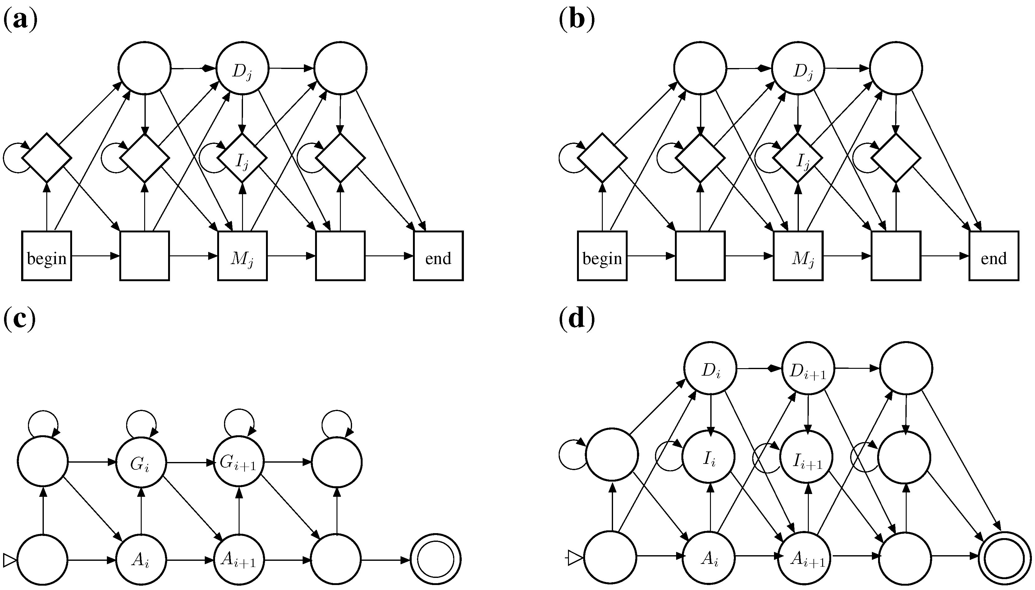
• HMMs are normally described as Moore machines, which emit symbols on states, independent of transitions. In our grammar, "emissions" are associated with the transitions: symbol $s_i$ is generated on transition into from $S_i$ to $S_{i+1}$. In this sense, they are closer to Mealy machines.
• In a profile HMM, the target model is built from a multiple sequence alignment, rather than from a single sequence. In the target S, the “characters” now are columns from that alignment. Each matching state of the HMM (square state) is a position in the target sequence.
• Scoring parameters in HMMs are position-specific. This implies that the scoring algebra of the ICORE should take into account the position in the core term: In $\mathtt{rep}(s_i,b,x)$, column $s_i$ is represented simply by i, which is used to look up the score parameter for this position.

Figure 3. (a) Graphical representation of a profile HMM (left, source: [20], Figure 5.2.); (b) dependency graph for grammar MatchAffi_S; (c) for MatchOsci_S; and (d) MatchTrace_S.

Figure 3. (a) Graphical representation of a profile HMM (left, source: [20], Figure 5.2.); (b) dependency graph for grammar MatchAffi_S; (c) for MatchOsci_S; and (d) MatchTrace_S.

Looking at HMMs as special ICOREs sheds a new light on profile HMMs. For example, the textbook model allows for state sequences such as $D_1{I}_1{I}_1{I}_1{D}_2{D}_3{I}_3{I}_3{I}_3...$, which is but one of many different transition paths for the same situation: an adjacent group of (say) 6 insertions and 3 deletions has $\left(\genfrac{}{}{0pt}{}{6+3}{3}\right)$ state paths, and their probabilities must be added to obtain the correct probability of this situation. Returning a most likely state path is meaningless in this situation. Our MatchSeq_S, derived from EditDistance, shares this undesirable property.

But starting from an ICORE using grammar AffiTrace instead, we obtain alternative profile HMMs with better properties. Consider Figure 3d: a matcher derived from AffiTrace inherits the avoidance of such ambiguity, by enforcing the convention that deletions must precede insertions whenever they are not separated by a replacement. With this architecture, we have a state transition sequence $A_1{D}_1{D}_2{D}_3{I}_3{I}_3{I}_3{I}_3{I}_3{I}_3$ as the only representation of the critical situation, and it collects the probability of this situation in a single state path.

6. ICOREs for RNA Secondary Structure Analysis

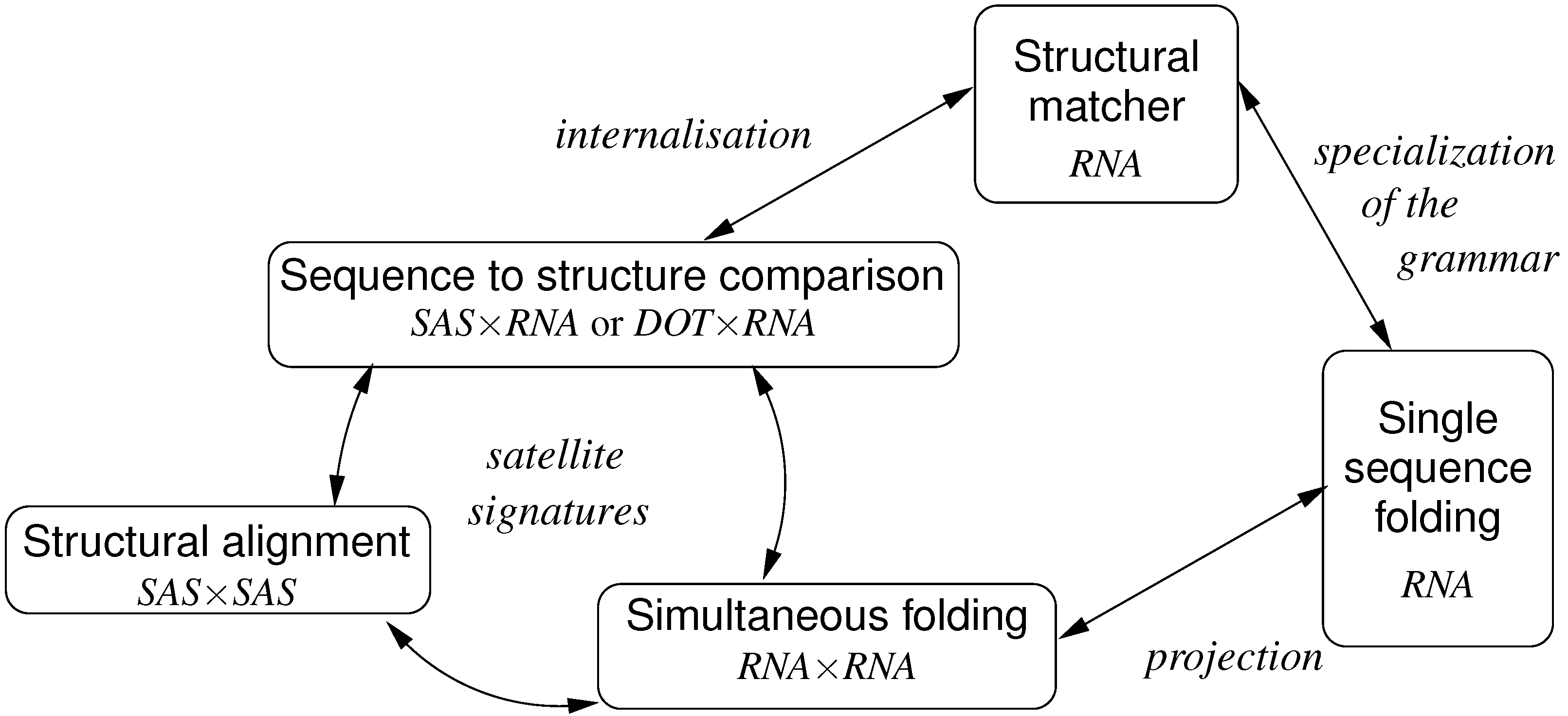
6.1. RNA Structure Analysis Overview

RNA is the active form of genetic information. In contrast to DNA, RNA is a single chain molecule, and with its backbone bending back onto itself, it forms structure that is responsible for an enormous variety of biological functions. Certain bases arranged on the backbone may form hydrogen bonds, and this set of base pairs, abstracting from their spatial arrangement, is called the secondary structure of an RNA molecule. A tiny example is shown in Figure 4. Computational analysis of RNA gives rise to a number of problems related both to the sequence and the secondary structure of the molecule: structure prediction, structure comparison, structural motif search, and more. The purpose of this section is to show how all these problems can be adressed in an unified way with ICOREs. Relationships between the different problems become explicit when formulated as ICOREs, while in the traditional dynamic programming recurrences, they are buried by detail.

Figure 4. Example of RNA secondary structure. This diagram shows a 2D representation of a secondary structure for the sequence "ACGACGGAUCUU" (left). This structure contains four base pairings: A-U, C-G, G-C and G-C. We also display its bracket-dot representation (middle), and its encoding within the satellite signature RNA, SAS and DOT (right).

Figure 4. Example of RNA secondary structure. This diagram shows a 2D representation of a secondary structure for the sequence "ACGACGGAUCUU" (left). This structure contains four base pairings: A-U, C-G, G-C and G-C. We also display its bracket-dot representation (middle), and its encoding within the satellite signature RNA, SAS and DOT (right).

We begin with the simplest version of RNA structure prediction, starting from a single sequence. This also serves to introduce readers without a bioinformatics background to RNA structure problems. We then continue with the problem of RNA structural alignment, where two sequences with a known or to-be-predicted structure are aligned for best agreement of sequence and structure. This problem will serve as a general template for subsequent problems: simultaneous folding and alignment of RNA sequences, and sequence to structure comparison.

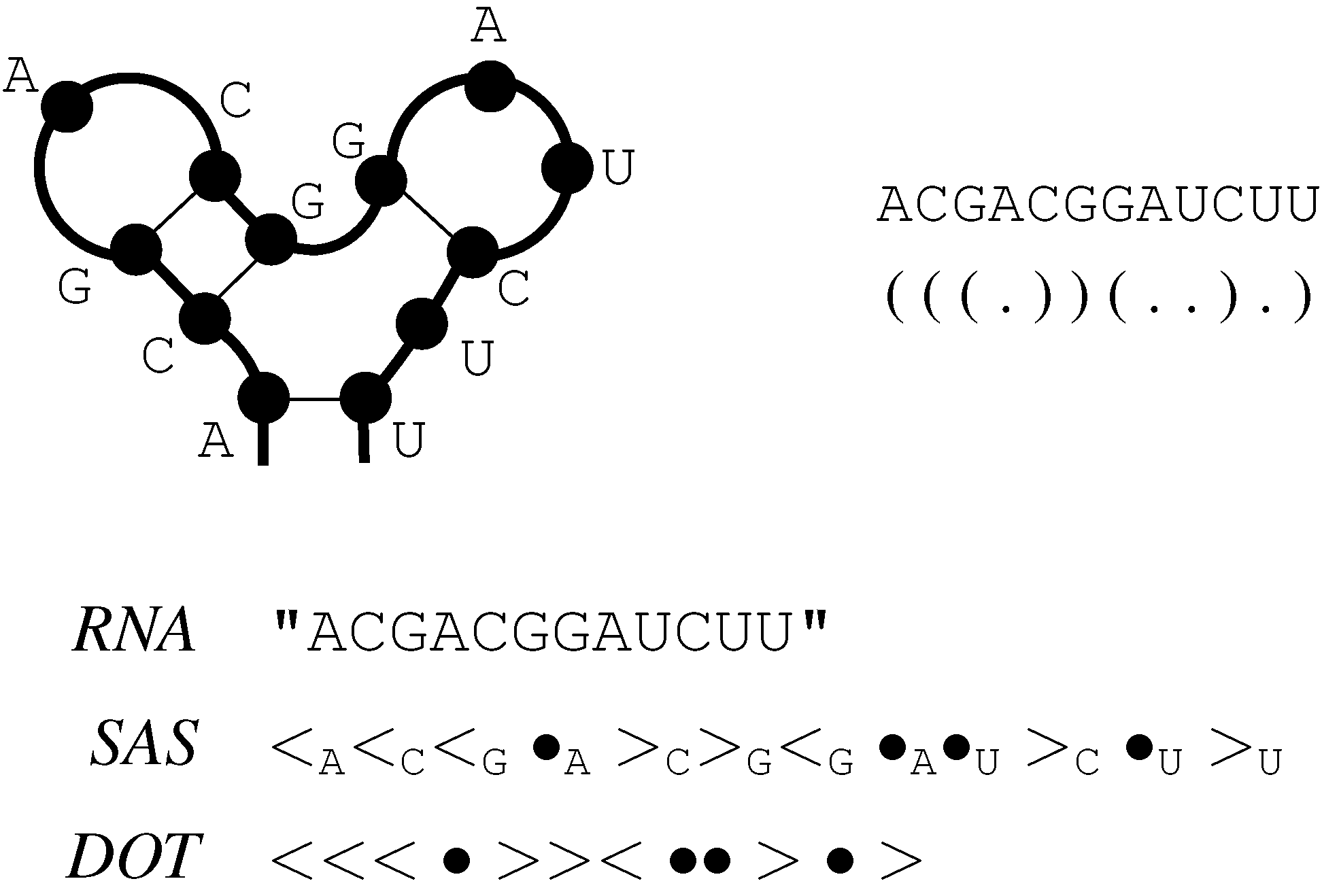
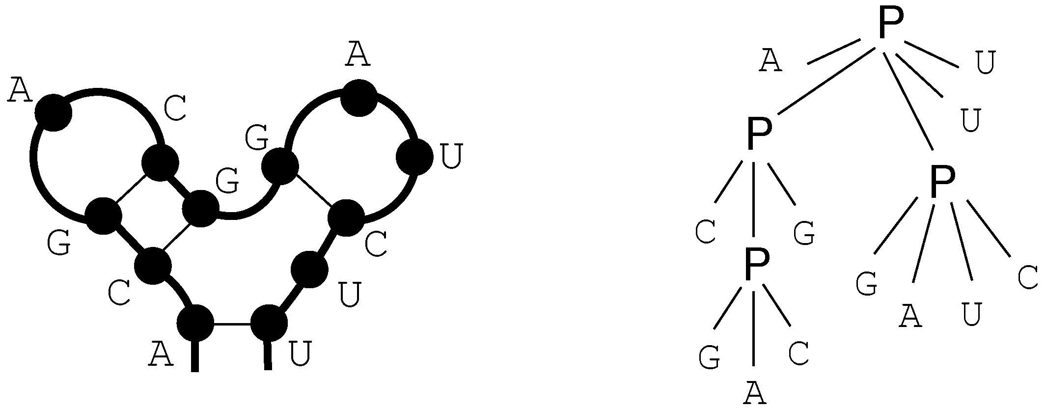
6.2. Satellite Signatures for RNA Sequences and Structures

Before proceeding, we introduce the three satellite signatures that will be shared by the upcoming ICOREs. Input to our problems will be one or more RNA sequences, with or without secondary structure indicated. The first signature RNA is used to denote plain sequences over the alphabet of RNA bases A(denine), C(ytosine), G(uanine), and U(racil).

Satellite signature RNA

  alphabet $\{\mathtt{A},\mathtt{C},\mathtt{G},\mathtt{U}\}$

  operators $\{\sim$, $\epsilon \}$

The second signature SAS describes an RNA sequence together with its secondary structure in a concise way. The name SAS stands for “structure-annotated RNA sequence”. ([This is closely related to, but not to be confused with “arc-annotated sequences”, which we will use in Figure 5. An arc indicates a base pair and knows its two end positions. In an SAS, you need a little parser to find the matching ${<}_{\mathtt{U}}$ for a given ${>}_{\mathtt{A}}$.]) Here, we consider only secondary structures without the so-called pseudoknots. This means that base pairs correspond to well-parenthesized expressions. The alphabet for sequences annotated with structure is the product of the well-known dot-bracket notation for secondary structures with the alphabet $\{\mathtt{A},\mathtt{C},\mathtt{G},\mathtt{U}\}$. Dots denote unpaired bases, while matching brackets indicate based pairs. Hence, this alphabet contains 12 novel character symbols. (In practice, one will use two strings of ASCII characters, one holding the base sequence, one holding the annotation. However, since their positions are strictly coupled, this is formally a one dimensional problem over an extended alphabet.)

Figure 5. Operators for edit operations in the core signature. Deletion of a base pair may remove both bases ($\mathtt{pair}\_\mathtt{del}$) or solely the 5’ or 3’ partner leaving the remaining partner as a bulge ($\mathtt{pairL}\_\mathtt{del}$ and $\mathtt{pairR}\_\mathtt{del}$). Symmetrically, we have all operators for insertion operations.

Figure 5. Operators for edit operations in the core signature. Deletion of a base pair may remove both bases ($\mathtt{pair}\_\mathtt{del}$) or solely the 5’ or 3’ partner leaving the remaining partner as a bulge ($\mathtt{pairL}\_\mathtt{del}$ and $\mathtt{pairR}\_\mathtt{del}$). Symmetrically, we have all operators for insertion operations.

Satellite signature SAS

  alphabet $\{{•}_{\mathtt{A}},{•}_{\mathtt{C}},{•}_{\mathtt{G}},{•}_{\mathtt{U}},{<}_{\mathtt{A}},{<}_{\mathtt{C}},{<}_{\mathtt{G}},{<}_{\mathtt{U}},{>}_{\mathtt{A}},{>}_{\mathtt{C}},{>}_{\mathtt{G}},{>}_{\mathtt{U}}\}$

  operators $\{\sim$, $\epsilon \}$

The third signature $DOT$ will serve for strings indicating structure without sequence information:

Satellite signature DOT

  alphabet $\{•,<,>\}$

  operators $\{\sim$, $\epsilon \}$

Figure 4 shows the usual two-dimensional representation for an RNA sequence, accompanied by its notation in bracket-dot format, and for the signatures RNA, SAS and DOT.

6.3. RNA Folding

Our first RNA-related ICORE is a version of the classical Nussinov algorithm which, given a single RNA sequence, predicts its secondary structure by maximizing the number of base pairs [22]. This problem is of dimension 1. The input is a plain sequence represented as a string from the satellite signature $RNA$, and the output is a secondary structure. We need a core signature $STR$ to describe such secondary structures. For that, we use four operators. Operator $\mathtt{mty}$ represents the empty structure, $\mathtt{pair}$ takes as input two letters and a substructure and builds a base pair around the latter, $\mathtt{single}$ takes as input one letter and adds it as an unpaired base to a structure, and $\mathtt{split}$ is for the concatenation of two structures, used when a structure branches as in Figure 4.

Example 4. Figure 6 shows a core term for the plain sequence "ACGACGGAUCUU". This core term represents the secondary structure displayed in Figure 4.  □

Figure 6. Core term for secondary structure of Figure 4.

Figure 6. Core term for secondary structure of Figure 4.

The grammar SecStr (see below) guarantees that this representation is unique. It uses a production of tree height 2 to make sure that core terms uniquely represent secondary structures, disallowing core terms such as $\mathtt{split}(\mathtt{mty},\mathtt{mty})$ Grammar SecStr does not impose a restriction on the two bases in $\mathtt{pair}(a,S,b)$, so the structure terms may also represent structures with non-standard base pairs. For the RNA folding problem, legal base pairing is enforced in the rules, where $\mathtt{basep}$ is a syntactic predicate defining legal base pairs. The standard definition is

$$\begin{array}{ccc}\hfill \mathtt{basep}(a,b)& =& \left\{\right(a,b)\in \{(\mathtt{A},\mathtt{U}),(\mathtt{U},\mathtt{A}),(\mathtt{C},\mathtt{G}),(\mathtt{G},\mathtt{C}),(\mathtt{G},\mathtt{U}),(\mathtt{U},\mathtt{G})\}\hfill \end{array}$$

to allow for canonical base pairs (Watson-Crick or wobble base pairs). By setting

$$\begin{array}{ccc}\hfill \mathtt{basep}(a,b)& =& \mathtt{TRUE}\hfill \end{array}$$

we would allow also non-canonical pairs and let the scoring makes the difference. This is commonly done in stochastic RNA family models, where non-standard base pairs are allowed with low probability.

The rewrite rules explain how to build the secondary RNA structure from the plain sequence: either by creating a base pair with $\mathtt{pair}$, or by adding a single base with $\mathtt{single}$, or by concatenating two structures with $\mathtt{split}$. Completed with some algebras, the resulting ICORE RNAfold is displayed on page 93.

We propose three algebras with ICORE RNAfold:

• Algebra BPmax implements base pair maximization as our objective function, as it is done in the Nussinov algorithm.
• Algebra DotPar serves to visualize predicted structures as strings in a dot-bracket notation. Used by itself in a call to RNAfold(DotPar, s), this algebra would enumerate the full candidate space for input s. Normally, it is used in a product with other algebras (cf. Section 8), where it reports optimal candidates.
• Algebra Prob assigns a probability score to each core term, such as it is done with stochastic context free grammars [20,23,24].

Algebra Prob deserves more comments. Stochastic context free grammars (SCFGs) allow to parse a string into (context free) structures of any kind, and a stochastic scoring scheme allows us to select the most likely parse for it, or to compute the probability sum over all parses.

The parameters ${\pi }_a$, ${\pi }_{ab}$, and ${\pi }_{split}$ reflect the probability of encountering an unpaired base a, a base pair $(a,b)$, and a structural split; they must be estimated from a set of training data. More sophisticated SCFGs will replace the grammar SecStr by a more refined grammar, leading to a larger number of parameters, but in principle, nothing else changes. Calling RNAfold with algebra $Prob$ an input sequence s and $\varphi =max$, we can find the most likely parse of sequence s, which indicates a structure of high likelihood. Since the grammar SecStr is semantically non-ambiguous [21,25] (i.e., each parse designates a different structure), this is also the most likely structure assigned to s under the given model. This is known as Viterbi scoring. Choosing $\varphi =sum$ instead, we obtain the overall probability of sequence s under the given model, summed up over all parses. This is also known as inside scoring.

6.4. Structural Alignment

Structural alignment is used to compare two RNA sequences taking into account both levels of information: sequence and secondary structure. Not only base sequences are aligned, using gaps as usual, but when two bases are aligned that are involved in base pairs, their respective partners must be aligned preferentially with each other, too. This condition cannot be met by simply aligning two sequences from the $SAS$ alphabet by the algorithms of Section 5. In fact, structural alignment gives rise to many interesting, related problems, and has attracted a large amount of research in RNA bioinformatics.

A commonly seen visualization of a structural alignment is given in Figure 7. Two sequences are annotated with different, but similar structures, and are aligned with respect to these structures. You may spot four gap symbols in this Figure, which mark three different situations and will score differently. The first gap (from the left) marks a G base inserted in the lower sequence. The second marks a C-G pair in the upper sequence, where the C residue has been lost in the lower sequence, while the G is still there and unpaired. The remaining two gap symbols mark a G-C pair in the upper sequence, where neither base has a counterpart in the lower sequence.

Figure 7. Example of a structural RNA alignment. Vertical bars indicate matching bases in the sequences. Note that the two structures are different, but similar.

Figure 7. Example of a structural RNA alignment. Vertical bars indicate matching bases in the sequences. Note that the two structures are different, but similar.

6.4.1. Core Signature and Grammar for Structural Alignment

A core signature for structural alignments must be elaborate enough to accommodate all these and similar situations, to allow for their independent scoring. We consider here the most general set of edit operations, such as introduced in [26], that is used with arc-annotated sequences and that allows for any kind of mutational event. Edit operations representing structural matches between single bases or base-pairings are $\mathtt{mty}$, $\mathtt{single}$, $\mathtt{split}$, and $\mathtt{pair}$. We re-use the names from signature STR, but note that $\mathtt{single}$ and $\mathtt{pair}$ now hold bases from both sequences as their arguments. For mismatches, we need edit operations for deletion and insertion of unpaired residues: $\mathtt{del}$ and $\mathtt{ins}$, which both have exactly the same semantics as in sequence alignment (Section 5). We must also allow that a base pair in one sequence may be not present in the other sequence, because one or both bases are missing or because the pair cannot be formed, as dictated by predicate $\mathtt{basep}$. These cases give rise to eight new operations, $\mathtt{pair}\_\mathtt{ins}$, $\mathtt{pair}\_\mathtt{del}$, $\mathtt{pairL}\_\mathtt{ins}$, $\mathtt{pairL}\_\mathtt{del}$, $\mathtt{pairR}\_\mathtt{ins}$, $\mathtt{pairR}\_\mathtt{del}$, $\mathtt{pairLR}\_\mathtt{ins}$, $\mathtt{pairLR}\_\mathtt{del}$. Therefore, we have a total of 12 edit operations (This does not account for $\mathtt{mty}$ and $\mathtt{split}$, as in the standard model. An edit operation where the left or right part of a split has been lost might well be useful. It has been overlooked in the edit model of [26], probably because the graphical representation of structures as arc-annotated sequences has no explicit representation for structural branching.), which are summarized graphically in Figure 5. Collecting the above cases, we arrive at a core signature STRAL with 14 operators.

In the definition of STRAL, $\mathcal{R}$ denotes the RNA alphabet $\{\mathtt{A},\mathtt{C},\mathtt{G},\mathtt{U}\}$, and StrAli is the (only) sort of terms from the core signature. Akin to grammar SecStr, the grammar for structural alignment, StructAli, should avoid ambiguous structure representations, and does so by using an extra non-terminal symbol P. The ICORE is presented on page 97.

Example 5. Consider the following structural alignment, presented in dot-bracket notation.

      ( . - - ) ( )

      A G - - U C G

      | |     | |

      A G C C U C A

      ( ( ) . ) . .

It is encoded by the core term

$c=\mathtt{split}\left(\mathtt{pair}\right(\mathtt{A},\mathtt{A},\mathtt{split}(\mathtt{pairL}\_\mathtt{ins}(\mathtt{G},\mathtt{G},\mathtt{mty},\mathtt{C}),\mathtt{ins}(\mathtt{C},\mathtt{mty}\left)\right),\mathtt{U},\mathtt{U}),\mathtt{pairLR}\_\mathtt{del}(\mathtt{C},\mathtt{C},\mathtt{mty},\mathtt{G},\mathtt{A})$ which satisfies

$${<}_{\mathtt{A}}{•}_{\mathtt{G}}{>}_{\mathtt{U}}{<}_{\mathtt{C}}{>}_{\mathtt{G}}{\leftarrow }^{*}c{\to }^{*}{<}_{\mathtt{A}}{<}_{\mathtt{G}}{>}_{\mathtt{C}}{•}_{\mathtt{C}}{>}_{\mathtt{U}}{•}_{\mathtt{C}}{•}_{\mathtt{A}}$$

□

Core signature STRAL

6.4.2. Structural Alignment in the Prism of Tree Alignment

Prior to [26], approaches to structural alignment were less refined and considered base pairs as a unit which could only be deleted or inserted [27]. This amounts to considering RNA secondary structures as ordered rooted trees: each base pair is an internal node, and each single base is a leaf. Hence, a situation such as our $\mathtt{pairL}\_\mathtt{del}$, resulting from a single point mutation in the genomic sequence, had to be modeled and scored as two changes, a pair deletion plus a single base insertion. This more restricted model is obtained from ICORE StructAli simply by dropping rules $\left({\alpha }_9\right)-\left({\alpha }_{14}\right)$. (Note that we need not formally restrict the core signature to take out specific edit operations. Since they no longer show up in the rewrite rules, they are not part of the inverse image of the input sequences, and by Definition 4, they play no role in the search space.)

6.5. The Sankoff Algorithm for Simultaneous Alignment and Folding, with Variations

We now turn to the problem of simultaneous alignment and folding: We are given two plain RNA sequences, and the goal is to infer a conserved consensus structure. This problem makes sense when the two input sequences are assumed to be homologous. It was first addressed by Sankoff [5], and has given rise to many related problem formulations since then.

To design ICOREs for this new family of problems, we explain how the ICORE StructAli for structural alignment presented in Section 6.4 can be systematically modified to deal with plain RNA sequences whose secondary structure is not known.

6.5.1. Structural Alignment without Given Structures

How to transform an alignment between structure-annotated sequences into an alignment between sequences whose structure is to be guessed? Just let us eliminate structure annotation from the input of StructAli. The satellite signatures change from SAS to RNA, and we adjust the right-hand sides of the rewrite rules in consequence. We replace each symbol of $SAS$ of the form ${<}_a$, ${>}_a$, or ${•}_a$ with the symbol a from $RNA$. As the structure is no longer given, we impose legal base pairing by means of the predicate $\mathtt{basep}$ in the rewrite rules. Otherwise, the new rules are a literal copy from StructAli. This is what is done with ICORE SimultaneousFolding, presented on page 98. Operators of the core signature and the grammar are left untouched.

Let us now study two simplifications of this new ICORE.

6.5.2. Exact Consensus Structure

If we restrict SimultaneousFolding to rules $\left({\beta }_1\right)-\left({\beta }_4\right)$, only operators $\mathtt{mty}$, $\mathtt{single}$, $\mathtt{split}$, and $\mathtt{pair}$ are authorized. We get an ICORE which we call ExactConsensusStructure, where the two sequences are folded into the same structure, which is their exact consensus structure selected from the intersection of the folding spaces of the two sequences. No insertions and deletions are allowed, and hence, both sequences must be of the same length. If their lengths differ, the search space of exact consensus structures will simply be empty.

Example 6. What are the possible consensus structures of sequences "GAUA" and "CAGU"? We find that there are (only) three core terms that rewrite to our pair of example sequences:

$$\mathtt{split}\left(\mathtt{pair}\right(\mathtt{G},\mathtt{C},\mathtt{single}(\mathtt{A},\mathtt{A},\mathtt{mty}),\mathtt{U},\mathtt{G}),\mathtt{single}(\mathtt{A},\mathtt{U},\mathtt{mty}\left)\right)$$

$$\mathtt{single}(\mathtt{G},\mathtt{C},\mathtt{single}(\mathtt{A},\mathtt{A},\mathtt{split}\left(\mathtt{pair}\right(\mathtt{U},\mathtt{G},\mathtt{mty},\mathtt{A},\mathtt{U}),\mathtt{mty})\left)\right),\mathrm{and}$$

$$\mathtt{single}(\mathtt{G},\mathtt{C},\mathtt{single}(\mathtt{A},\mathtt{A},\mathtt{single}(\mathtt{U},\mathtt{G},\mathtt{single}(\mathtt{A},\mathtt{U},\mathtt{mty}\left)\right)\left)\right)$$

which correspond to the following exact consensus secondary structures (in the same order, from left to right):

G A U A        G A U A       G A U A

( . ) .        . . ( )       . . . .

C A G U        C A G U       C A G U

For example, the first core term $c=\mathtt{split}\left(\mathtt{pair}\right(\mathtt{G},\mathtt{C},\mathtt{single}(\mathtt{A},\mathtt{A},\mathtt{mty}),(\mathtt{U},\mathtt{G})),\mathtt{single}(\mathtt{A},\mathtt{U},\mathtt{mty}\left)\right)$ rewrites as "GAUA"${\leftarrow }^{*}c{\to }^{*}$"CAGU". In contrast, the core term

$$c^{\prime }=\mathtt{single}(\mathtt{G},\mathtt{U},\mathtt{split}(\mathtt{pair}(\mathtt{A},\mathtt{A},\mathtt{mty},\mathtt{U},\mathtt{G}),\mathtt{single}(\mathtt{A},\mathtt{U},\mathtt{mty})\left)\right)$$

fails to rewrite to the left satellite "CAGU", because the condition $\mathtt{basep}(\mathtt{A},\mathtt{G})$ in Rule (${\beta }_4$) fails. ☐

6.5.3. The Sankoff Algorithm

Adding back in rules $\left({\beta }_5\right)-\left({\beta }_6\right)$, we go one step further and consider alignments with insertion and deletion of unpaired residues in the alignment, such as the two alignments below.

G-UCC                     -GUCC

(.)..                     .(..)

AUUG-                     AUU-G

This is exactly the model used in the Sankoff algorithm. Intuitively, it merges the ideas of sequence alignment with those of RNA structure prediction [5]. With the ICORE formalism, this is literally what happens: We obtain the ICORE Sankoff by augmenting ExactConsensusStructure with the indel rules from EditDistance.

Example 7. For example,

$$t=\mathtt{split}\left(\mathtt{pair}\right(\mathtt{G},\mathtt{A},\mathtt{ins}(\mathtt{U},\mathtt{mty}),\mathtt{U},\mathtt{U}),\mathtt{single}(\mathtt{C},\mathtt{G},\mathtt{del}(\mathtt{C},\mathtt{mty})\left)\right)$$

represents the structural alignment on the left above. We find $“\mathtt{GUCC}”{\leftarrow }^{*}t{\to }^{*}“\mathtt{AUUG}”.$ We leave it to the reader to script the core term representing the structural alignment in the right. ☐

6.6. Sequence-to-Structure Alignment and RNA Family Modeling

The two preceding subsections have cast the structure alignment problem and the simultaneous folding problem in a unified approach. This opens the door to many variations of these themes, allowing any combination of input sequences, either plain RNA sequences from RNA or sequences including secondary structure information from SAS, or even DOT if we have a structure model without sequence information.

We examine here in more detail the sequence-to-structure alignment problem: One input is a target structure–from SAS or DOT –, the other a plain sequence from RNA. We want to know how well the plain RNA sequence can fold into the target structure. This problems comes in two variations: When the structure can be given as an input parameter, we call this a generic structural matching problem. If the target structure is fixed, it can be hard-coded into the matcher, which then takes the form of an RNA motif matcher. This RNA motif matcher can be used to define an RNA family model.

6.6.1. A Generic Structure Matcher

A generic structure matcher allows us to fold a plain sequence into a target structure, using the full range of edit operations available in the core signature $STRAL$. For that, we start from ICOREs SimultaneousFolding and StructAli. Recall that the rewrite rules of SimultaneousFolding reduce a core term to two plain RNA sequences, while StructAli reduce the same term to two structure-annotated sequences. To obtain an ICORE for the sequence-to-structure matching problem, all we have to do is take half of each: rules of StructAli for rewriting to the target structure t, and rules of SimultaneousFolding for rewriting to the RNA sequence s. We call this new ICORE $S2Sgeneric$ (page 101). With inputs t from SAS and s from RNA, it will predict a structure for s that aligns best (however defined by algebra Score) to the t. Changing the first satellite signature from $SAS$ to $DOT$ (and replacing ${•}_a$ with • etc. in the rules) would solve the same task for a target that is a pure structure without an associated sequence.

6.6.2. Generic Exact Structure Matching

If we restrain ICORE S2Sgeneric to rules $\left({\gamma }_1\right)-\left({\gamma }_4\right)$, we get an ICORE S2Sexact for the exact structure match problem: does the RNA sequence fit exactly into the target structure? Being a little less strict, and keeping also rules $\left({\gamma }_5\right)-\left({\gamma }_6\right)$, we would allow gaps with respect to unpaired bases, while still all base pairs in the target must be formed in the query.

Example 8. Consider the core term

$$\begin{array}{ccc}\hfill t& =& \mathtt{split}(\mathtt{pair}(\mathtt{C},<,\mathtt{single}(\mathtt{A},•,\mathtt{mty}),\mathtt{G},>),\mathtt{ins}(\mathtt{C},t^{\prime })),\mathrm{where}\hfill \\ \hfill t^{\prime }& =& \mathtt{split}\left(\mathtt{pair}\right(\mathtt{A},<,\mathtt{split}\left(\mathtt{pair}\right(A,<,\mathtt{single}(\mathtt{G},•,\mathtt{mty}),\mathtt{U},>),\mathtt{mty}),(U,>)),\mathtt{mty})\hfill \end{array}$$

We find

$$“\mathtt{CAGCAAGUU}”{\leftarrow }^{*}t{\to }^{*}“<•><<•>>”$$

Note in detail that the second C is considered an insertion in the query. ☐

6.6.3. From Generic to Hard-Coded Structure Matching

In the previous subsection, we spoke of generic sequence and structure matching, because we used ICOREs of dimension 2, where both the RNA plain sequence and the target secondary structure are given as inputs. Structural matchers such as produced by the tools RNAMotif or Locomotif [28,29] only take a single parameter, the query sequence, while the structure to be matched against is hard-coded in the program (for better efficiency). We show how to design two types of specialized matcher ICOREs of dimension 1, using the internalization mechanism introduced in Subsection 5.3 for sequence analysis.

For the two following sections, let the target structure be $r={<}_{\mathtt{A}}{<}_{\mathtt{G}}{•}_{\mathtt{U}}{>}_{\mathtt{C}}{•}_{\mathtt{G}}{>}_{\mathtt{U}}{<}_{\mathtt{C}}{>}_{\mathtt{G}}{•}_{\mathtt{A}}$. A hard-coded matcher for r re-uses the constituents of the generic matcher of dimension 2, but replaces the grammar by a specific grammar, that is derived by parsing r with SecStr, and keeping track of which rules are used to produce which symbols in r. Let us explicitly annotate symbols in r with their position in superscript:

$$r={<}_{\mathtt{A}}^1{<}_{\mathtt{G}}^2{•}_{\mathtt{U}}^3{>}_{\mathtt{C}}^4{•}_{\mathtt{G}}^5{>}_{\mathtt{U}}^6{<}_{\mathtt{C}}^7{>}_{\mathtt{G}}^8{•}_{\mathtt{A}}^9$$

6.6.4. A Structural Matcher for Exact Search

For sake of clarity, we first head for the hard-coded version of the simple ICORE S2Sexact, that contains only four rules, $\left({\gamma }_1\right)-\left({\gamma }_4\right)$. The goal is to construct a grammar that restricts the search space to all and only the core terms that rewrite to r on the first satellite. Given this grammar, there will no longer be a need to rewrite a core term to r, and hence we will be able to eliminate altogether the first satellite and the rewrite rules that produce it. We start from the grammar StructAli, and ignore all rules that deal with deletions and insertions, as we are heading for an exact matcher. This leaves us with four rules, which reduce to three after “inlining” the nonterminal symbol P for simplification. The grammar now is simply

$$\begin{array}{ccc}S\hfill & \to \hfill & \mathtt{single}(a,c,S)\left|\mathtt{split}\right(\mathtt{pair}(a,c,S,b,d),S\left)\right|\mathtt{mty}\hfill \end{array}$$

As r has 9 residues, we create 10 copies of this grammar, which use 10 non-terminal symbols, indexed by the positions in r. This gives the grammar template

$$\begin{array}{ccc}{S}_i\hfill & \to \hfill & \mathtt{single}(a,c,S_{i+1})\left|\mathtt{split}(\mathtt{pair}(a,c,S_{i+1},b,d),S_{j+1})\right|\mathtt{mty}\hfill \end{array}$$

where j is determined as the position of the closing base partner of position i. Now we specialize this grammar template to retain productions that can be applied in a successful derivation of residue i in r, and then drop whatever refers to the first satellite input. For each symbol ${•}_a^i$ in r, we have a production

$$S_i\to \mathtt{single}(a,c,S_{i+1})$$

and for each pair of matching brackets ${<}_a^i$ and ${>}_b^j$ in r, we have a production

$$S_i\to \mathtt{split}(\mathtt{pair}(a,c,S_{i+1},b,d),S_{j+1})$$

This leads to the grammar and ICORE named Match_S2S_r for the sequence-to-structure alignment problem with target r, that is displayed on page 103. For clarity, we have added the position of each character in r in a superscript in the grammar.

Example 9. With ICORE Match_S2S_r, we find that there is some core term t such that

$$t{\to }^{*}“\mathtt{GGUCUCAUG}”$$

while there is no core term $t^{\prime }$ such that

$$t^{\prime }{\to }^{*}“\mathtt{AGUCUCAUG}”$$

☐

The core terms generated by the grammar of Match_S2S_r contain all the sequence information about the target structure, and so, a core signature algebra can implement position and sequence specific scoring. If no scoring depending on the sequence content of the internalized target is desired, the ICORE can be simplified by not reproducing the residues of the target. The core signature simplifies from $STRAL$ to $STR$, and we obtain an new ICORE, Match_S2S_r’ presented on page 104. In this simplified form, this ICORE is the same as RNAFold (page 93), except for the grammar. Naturally–all we do is predicting a structure for a plain RNA sequence, restricted to match the target. This ICORE, without the provision for target specific scoring, could also have been derived from RNAfold directly.

6.6.5. A Structural Matcher for Covariance Models

Covariance models (CMs) [20,30,31] describe families of RNA sequences, based on sequence similarity and structure conservation. A group of related sequences is aligned, a consensus structure is determined, and a model is built with a particular choice of architecture. Stochastic parameters are trained from the data. Model and parameters are applied to short query sequences, or in local search mode to scan whole genomes, to find additional family members. New members can be included into the set that defines the model, and parameters re-trained. Included sequences constitute the core of the model, called the “seed alignment” in Rfam terminology [32], while all known sequences that match the model above a certain threshold score constitute the “full aligment”. So, there it a lot more going on than just solving a straighforward combinatorial optimization problem–but at the heart of the approach, there is the task of aligning a plain RNA sequence s to a target structure r.

In contrast to the exact matcher Match_S2S_r, a covariance model allows for deletions from the target structure, as well as for insertions in the RNA sequence. However, it does not allow for all possible operations from the core signature $STRAL$. Insertions in the RNA sequence are always considered unpaired (because for features not present in the model, one cannot train parameters). Hence, we will make no use of $\mathtt{pair}\_\mathtt{ins}$, $\mathtt{pairLR}\_\mathtt{ins}$, $\mathtt{pairL}\_\mathtt{ins}$, and $\mathtt{pairR}\_\mathtt{ins}$. The operator $\mathtt{pairLR}\_\mathtt{del}$ also goes away: It stands for a case where two unpaired bases are aligned to a base pair in the target. In covariance models, these bases are always considered paired, and scored with a low probability if they cannot legally form a pair. So operator $\mathtt{pair}$ already takes care of this case. Inlining non-terminal P as before, this reduces grammar StructAli to the following productions.

$$\begin{array}{ccccc}& S^{*}& \to \hfill & & \mathtt{single}(a,c,S)\hfill \\ & & & |\hfill & \mathtt{mty}\hfill \\ & & & |\hfill & \mathtt{del}(a,S)\hfill \\ & & & |\hfill & \mathtt{ins}(c,S)\hfill \\ & & & |\hfill & \mathtt{split}\left(\mathtt{pair}\right(a,c,S,b,d),S)\hfill \\ & & & |\hfill & \mathtt{split}(\mathtt{pair}\_\mathtt{del}(a,S,b),S)\hfill \\ & & & |\hfill & \mathtt{split}(\mathtt{pairL}\_\mathtt{del}(a,c,S,b),S)\hfill \\ & & & |\hfill & \mathtt{split}(\mathtt{pairR}\_\mathtt{del}(a,S,b,d),S)\hfill \end{array}$$

For the moment, this is a generic matcher, with some edit operations disabled. To proceed to a covariance model, the target structure must be internalized. All variables (a and b in the grammar above) refering to the structure input will disappear. Applying the same internalization construction as with Match_S2S_r, we obtain from ICORE S2Sgeneric a specific matcher CovarianceModel_r. We use the same target structure r as in the previous example.

Example 10. Consider sequence $s="\mathtt{GUCUCAGUG}"$. It can be aligned to structure $r=``<<•>•><>•"$ in manifold ways such as

$\mathtt{G}$-$\mathtt{U}$$\mathtt{C}$$\mathtt{U}$$\mathtt{C}$$\mathtt{A}$$\mathtt{G}$$\mathtt{U}$$\mathtt{G}$ <<•>•><−>•

$\mathtt{G}$$\mathtt{U}$$\mathtt{C}$−−$\mathtt{U}$$\mathtt{C}$$\mathtt{A}$$\mathtt{G}$$\mathtt{U}$$\mathtt{G}$ <<•>•>-<−>•

$\mathtt{G}$$\mathtt{U}$$\mathtt{C}$$\mathtt{U}$$\mathtt{C}$$\mathtt{A}$−$\mathtt{G}$$\mathtt{U}$$\mathtt{G}$− -<-<•>•><>•

The core term expressing the leftmost alignment of the query s to the covariance model CovarianceModel_r derived from r is

$$t=\mathtt{split}(t^{\prime },\mathtt{split}\left(\mathtt{pair}(\mathtt{A},\mathtt{del}(\mathtt{G},\mathtt{mty},\mathtt{U}),\mathtt{single}(\mathtt{G},\mathtt{mty}))\right))\mathrm{where}$$

$$t^{\prime }=\mathtt{pair}(\mathtt{G},\mathtt{split}(\mathtt{pairL}(\mathtt{single}(\mathtt{U},\mathtt{mty},\mathtt{C}),\mathtt{single}(\mathtt{U},\mathtt{mty})),\mathtt{C})$$

☐

The above ICORE describes the search space of a specific covariance model. Now let us turn to scoring core terms. Note that even after all sequence information from r is eliminated, the grammar still “knows” (by the subscripted non-terminal symbols) the positions in the target structure to which a part of the query is aligned. For position specific scores, this information should be passed on to the scoring functions. The operator pair, for example, is implemented in a stochastic algebra (cf. Section 6.3) as

$$\begin{array}{ccc}\hfill \mathtt{pair}(a,x,b)& =& x*{\pi }_{ab}\hfill \end{array}$$

It is used with $S_1,S_2$, and $S_7$ in the specialized grammar. From the parameter estimation, we obtain (potentially) different probabilities ${\pi }_{ab}^1,{\pi }_{ab}^2$, and ${\pi }_{ab}^7$ for these residues. Different uses of $\mathtt{pair}$ must be able to resort to these different parameters. Such position-specific scoring is accommodated by extending the operators of the core signature by a position parameter, which is supplied when the core term is constructed. The definition of $\mathtt{pair}$ changes to

$$\begin{array}{ccc}\hfill \mathtt{pair}(i,a,x,b)& =& x*{\pi }_{ab}^i\hfill \end{array}$$

and the same applies to all other operators of the core signature. As a general technique, this extra parameter keeps signatures small and accommodates the requirements of position specific scoring.

Example 11. The core term t of Example 10, now with position information, becomes

$$t=\mathtt{split}(1,t^{\prime },\mathtt{split}(7,\mathtt{pair}(7,\mathtt{A},\mathtt{del}(8,\mathtt{G},\mathtt{mty}\left(8\right)),\mathtt{U}),\mathtt{single}(9,\mathtt{G},\mathtt{mty}\left(10\right))\mathrm{where}$$

$$t^{\prime }=\mathtt{pair}(1,\mathtt{G},\mathtt{split}(2,\mathtt{pairL}(2,\mathtt{single}(3,\mathtt{U},\mathtt{mty}\left(4\right),\mathtt{C}),\mathtt{single}(5,\mathtt{U},\mathtt{mty}\left(6\right))),\mathtt{C})$$

☐

However, often in practice when data are scarce, to avoid overfitting, parameters are tied together and become less position-specific. S2SGeneric may be called for with parameters trained from a similar structure $r^{\prime }$ and a background sequence composition. This can be done, in principle, even before family members of structure r are known. S2SGeneric may be an interesting research topic, and not just an intermediate step between the Sankoff algorithm and bona fide covariance models.

6.7. Conclusion on ICOREs for RNA Analysis

In this section, we have proposed ICOREs for a variety of RNA problems. All those ICOREs exhibit common features and can be derived systematically : They use the same core signatures, the same rewrite rules, or subsets thereof. Doing this, we have also shown that several well-known formalisms appear as special cases of our framework. Figure 8 gives a panoramic overview of the five main problems addressed in the section, and Figure 9 show the links that exist between the ICORE specifications of problems.

This way of seeing things also opens some new pespectives. Let us return to the full ICORE SimultaneousFolding, introduced in Subsection 6.4. With its full set of rules $\left({\beta }_1\right)-\left({\beta }_{14}\right)$, we have combined the Sankoff approach with the full edit model. What is such a generic RNA aligner good for? Its search space is the set of all possible structural alignments of two (yet unfolded) RNA sequences. It would return the two structures that allow for the optimal structural alignment. No model of this generality has been studied in the literature. It appears promising, although not trivial, as the two optimization criteria, individual structure quality versus structure and sequence agreement, must be balanced in a new and careful way. For structure quality, the thermodynamic model used in structure prediction could be employed. Biologically, this idea has a strong appeal: the consensus structure, as we compute it with present-day approaches, is a fictitious entity, whereas each RNA molecule folds and operates individually, and will often produce base pairings consistent with, but not part of the consensus structure. The new approach can deliver two structures that fold well, agree well, but need not be identical, and these may come closer to biological reality.

Figure 8. Overview of all RNA related problems adressed in Section 6. These problems are classified according to the edit operations they use (column on the left) and to the kind of inputs. For each problem, we indicate meaningful restrictions that are detailed in the text.

Figure 8. Overview of all RNA related problems adressed in Section 6. These problems are classified according to the edit operations they use (column on the left) and to the kind of inputs. For each problem, we indicate meaningful restrictions that are detailed in the text.

Figure 9. Relationships between our five main RNA problems.

Figure 9. Relationships between our five main RNA problems.

As for the problem of structural matching, with ICORE S2Sgeneric in Subsection 6.6, we have seen that fixing the first input to a target structure, disregarding base pair insertion, and internalization leads to ICORE CovarianceModel_r, which exhibits the architecture of covariance models. Such models are used today to define structural RNA family models. Reverting this view, S2Sgeneric can be seen as a more general family model builder. Is has the following novel aspects: (i) we can use it with a combination of scoring schemes, not necessarily stochastic; (ii) we can allow for structured insertions in the query, e.g., an extra stem of a certain size range; and (iii) we can internalize t to a different extent, using for example a structural skeleton, but with sequence motifs supplied upon search time. An approach of this generality has not been studied in the literature. As with SimultaneousFolding, our ICORE only gives the definition of the search space–the challenge of providing a meaningful combination of scoring criteria remains open. Note also that the ICOREs presented here are a global matchers, trying to fold their complete input into the target structure. To obtain localized versions, which locate a subsequence matching the target inside a longer RNA sequence, the operators and rules introduced for local sequence search in Section 5.2.3. can be re-used.

7. Tree Comparison and Related Problems

In this section, we consider problems on ordered, labeled trees. There are two main paradigms to compare such trees: edit distance and alignment. We encode both of them in ICORE framework, and show how they can combine. We also address the question of affine gap models. Finally, we shall generalize the classical, atomic model of tree comparison towards a more expressive model, where tree edit operations can be formulated as domain-specific bi-directional rewrite rules.

7.1. Notations and Signatures

A tree has a root node and a forest of subtrees, a forest is a (possibly empty) sequence of trees. Problems on trees and forests recursively imply each other, and must be solved jointly. We follow the tradition and simply speak of problems on trees.

In the classical formulation, tree nodes carry labels without any meaning. In particular, they have no fixed arity or argument types. This convention is strictly tied to the classical tree edit model, where a node can be inserted or deleted anywhere in a tree. In tree languages over a signature, as we used so far, this would result in a violation of the corresponding operator’s arity. Our trees with typed operators and fixed arities require a more elaborate model, and we will look at them in Section 7.5.

For the moment, we adhere to the classical formulation, where nodes carry arbitrary labels. To accommodate this in our rewriting framework, we will treat all node labels as unary operators, and represent trees like $a(x,y,z)$, $a\left(x\right)$, and a as $a(x\sim y\sim z)$, $a\left(x\right)$, and $a\left(\epsilon \right)$, respectively. Forests are built from trees by the associative binary operator ∼, such that $a\sim (b\sim c)=a\sim b\sim c=(a\sim b)\sim c$. Given a set F of node labels, our satellite signature to represent trees will be

Satellite signature $TREE$

$$\begin{array}{cccccc}\hfill \epsilon & :& & \to & Tree\hfill & \text{empty forest}\hfill \\ \hfill f& :& \hfill Tree& \to & Tree\hfill & \text{node label},\mathrm{for}f\in F\hfill \\ \hfill \sim & :& \hfill Tree\times Tree& \to & Tree\hfill & \text{concatenation of subtree forests}\hfill \end{array}$$

Our first core signature is designed to represent arbitrary tree alignments. The core terms representing tree alignments will use operators $\mathtt{rep},\mathtt{ins},\mathtt{del}$, while the operators from F used in the input signatures now play the role of a leaf label alphabet.

Core signature TreeAl

alphabet F – see remark above

$$\begin{array}{cccccc}\hfill \mathtt{rep}& :& \hfill F\times F\times Ali& \to & Ali\hfill & \text{node label replacement}\hfill \\ \hfill \mathtt{del}& :& \hfill F\times Ali& \to & Ali\hfill & \text{node deletion}\hfill \\ \hfill \mathtt{ins}& :& \hfill F\times Ali& \to & Ali\hfill & \text{node insertion}\hfill \\ \hfill \mathtt{mty}& :& & \to & Ali\hfill & \text{empty tree alignment}\hfill \\ \hfill \sim & :& \hfill Ali\times Ali& \to & Ali\hfill & \text{subforest concatenation}\hfill \end{array}$$

The core signature uses an operator ∼ for concatenating forests of sub-alignments.

7.2. Tree Alignment

This section is devoted to Jiang’s classical tree alignment algorithm [27], and its more recent variants. Tree alignment is not to be confused with the tree edit distance problem, which is covered in Section 7.3. For the relationship between these (and other) modes of tree comparison, see [33]. The tree alignment problem accepts two trees and constructs a common supertree which is optimal under some scoring scheme.

7.2.1. Classical Tree Alignment

The ICORE TreeAlign is given on page 111. Our simple scoring algebra TreeSimilarity uses additive similarity scoring, parameterized by a weight function w for replacements, and gap penalties δ and γ for insertions and deletions.

Example 12. Consider the core term $t=$

$$\mathtt{rep}(a,a,(\mathtt{del}(e,\mathtt{rep}(b,b,\mathtt{mty})\sim \mathtt{del}(c,\mathtt{mty}\left)\right)\sim \mathtt{ins}(f,(\mathtt{ins}(c,\mathtt{mty})\sim \mathtt{rep}(d,d,\mathtt{mty})\left)\right)\left)\right)$$

We find

$$a(e(b,c),d)=a\left(\left(e((b\sim c)\sim d)\right)\right){\leftarrow }^{*}t{\to }^{*}a(b\sim f(c\sim d))=a(b,f(c,d))$$

and

$$\mathrm{TREESIMILARITY}\left(t\right)=2\delta +2\gamma +w(a,a)+w(b,b)+w(d,d)$$

□

The correspondence between sequence and tree alignment is clearly expressed in ICOREs EditDistance and TreeAlign. A tree which does not branch represents a sequence, e.g., $a\left(b\right(c\left(d\right(\epsilon \left)\right)\left)\right)$ represents the string "abcd". In this case, rule (1) is not needed, and the other rules of ICORE TreeAlign are the same as in SeqAlign, modulo the change of representation. Alternatively, we can represent the sequence "abcd" as a forest of leaves, $a\left(\epsilon \right)\sim b\left(\epsilon \right)\sim c\left(\epsilon \right)\sim d\left(\epsilon \right)=a\left(\epsilon \right)\sim \left(b\right(\epsilon )\sim (c\left(\epsilon \right)\sim d\left(\epsilon \right)\left)\right))$. Two such forests give rise to alignments of the form $\mathtt{rep}(a,a^{\prime },\mathtt{mty})\sim \mathtt{del}(b,\mathtt{mty})\sim \cdots$, rewriting to the left to $a\left(\epsilon \right)\sim b\left(\epsilon \right)\sim \cdots$. Rewrite rules 1–1 are always combined with an application of 1. Integrating this step in the other rules, we obtain the rules

$$\begin{array}{ccc}\hfill f\left(\epsilon \right)\sim X\leftarrow & \mathtt{rep}(f,g,\mathtt{mty})\sim X& \to g\left(\epsilon \right)\sim X\hfill \end{array}$$

(1)

$$\begin{array}{ccc}\hfill f\left(\epsilon \right)\sim X\leftarrow & \mathtt{del}(f,\mathtt{mty})\sim X& \to X\hfill \end{array}$$

(2)

$$\begin{array}{ccc}\hfill X\leftarrow & \mathtt{ins}(f,\mathtt{mty})\sim X& \to f\left(\epsilon \right)\sim X\hfill \end{array}$$

(3)

$$\begin{array}{ccc}\hfill \epsilon \leftarrow & \mathtt{mty}& \to \epsilon \hfill \end{array}$$

(4)

which again, modulo the change of representation, resemble those of ICORE EditDistance.

7.2.2. Tree Alignment with Affine Gap Scoring

Tree alignment with affine gap scoring transfers the scoring models presented in Subsection 5.1 from pairwise sequence alignment to tree alignment. The difference is that the problem splits up in several variants because there are different ways to define a gap in a tree, all of which may be justified in a particular application.

This variety is a good example to see how the components of ICOREs cooperate in a modular fashion. The core signature captures affine scoring and the rewrite rules define the mapping between (all possible) core terms, i.e., alignments, and their input trees. These components remain the same, while different grammars come in to capture the different gap models which have been studied in the literature.

Core signature and rewrite rules for composite gap scoring. Starting from ICORE TreeAli with its atomic gap model, we first need to extend the core signature to distinguish gap openings from extensions, and describe suitable rewrite rules. We collect them in an ICORE template named TreeAliGeneric on page 113.

Figure 10. Gaps for tree comparison.

Figure 10. Gaps for tree comparison.

TreeAliGeneric is to be extended with different grammars, according to the type of gap considered. In the literature, we can find a variety of ways to define composite gaps in a tree. We review four of them, which are illustrated in Figure 10: (arbitrary) subtrees, complete subtrees, (arbitrary) subforests, and complete subforests. Let T be a tree. A subtreet of T is a set of nodes of T satisfying the two conditions: all the nodes of t have a lowest common ancestor, called the root of t, and for each node x of t, with the exception of the root, the parent of x belongs to t. A complete subtreet of T is a subtree such that for each node x of t, all descendants of x belong to t. A subforestF of T is a contiguous sequence of of subtrees. A complete subforest is a contiguous sequence of complete subtrees, which all share the same parent node.

Gaps as complete subtrees. In this mode, a gap node belongs to the same composite gap as its ancestor node. The fact that we require that gaps are complete subtrees means that it is not possible to continue an alignment in a subtree after a number of insertions and deletions. Such alignments are equivalent to edit scripts including no deletion, neither insertion of internal nodes. Chawathe proposed a quadratic algorithm for this problem with linear gap weights [34]. An alternative solution that allows for arbitrary gap weights is to be found in [35]. We present here a grammar CompleteSubtree for this kind of gap, which uses three non-terminal symbols: N(o gap), D(eletion) and I(nsertion).

Example 13. Consider the trees $a\left(b\right(c\sim f\left)\right)$ and $a\left(d\right(e\sim f\left)\right)$. The core term

$$t=\mathtt{rep}(a,a,t_1\sim t_2)\sim \mathtt{mty}\mathrm{where}$$

$$t_1=\mathtt{open}\_\mathtt{del}(b,\mathtt{del}(c,\mathtt{mty})\sim \mathtt{del}(f,\mathtt{mty})\sim \mathtt{mty})\sim \mathtt{mty}$$

$$t_2=\mathtt{open}\_\mathtt{ins}(d,\mathtt{ins}(e,\mathtt{mty})\sim \mathtt{ins}(f,\mathtt{mty})\sim \mathtt{mty})\sim \mathtt{mty}$$

represents the alignment where the subtree rooted by b is deleted, and the subtree rooted by d is inserted. Note that the grammar provides no way to align the two nodes labeled f once we deleted/inserted b and d. Also, a subtree below an $\mathtt{open}\_\mathtt{del}$ can host neither insertions nor further deletion openings, and vice versa for $\mathtt{open}\_\mathtt{ins}$.  □

Gaps as complete subforests. The preceding gap model can be extended by considering complete subforests, instead of complete subtrees. Here, a gap node can be the extension of a larger gap for two separate reasons - because its ancestor is a gap node (like for subtrees), or because its left sibling is a gap node. With this definition, any gap in the tree is a gap on the underlying sequence of leaves. In trees representing RNA secondary structure, any gap on the primary sequence that is consistent with the secondary structure (i.e., the gap does not break any base pair) is a complete subforest gap in the tree. Such gaps are implemented in [36,37,38].

Compared to CompleteSubtree, the grammar CompleteSubforest needs two additional symbols: E (sibling deletion) and J (sibling insertion).

Example 14. Consider the two trees $a(b\sim c(d)\sim e\sim f)$ and $a(b\sim f)$. In the complete subtree gap mode, the alignment requires two gaps:

$$t_1=\mathtt{rep}(a,a,\mathtt{rep}(b,b,\mathtt{mty})\sim \mathtt{open}\_\mathtt{del}(c,\mathtt{del}(d,\mathtt{mty}))\sim \mathtt{open}\_\mathtt{del}(e,\mathtt{mty})\sim \mathtt{rep}(f,f,\mathtt{mty}))\sim \mathtt{mty}$$

In the complete subforest mode, it requires only one gap:

$$t_2=\mathtt{rep}(a,a,\mathtt{rep}(b,b,\mathtt{mty})\sim \mathtt{open}\_\mathtt{del}(c,\mathtt{del}(d,\mathtt{mty}))\sim \mathtt{del}(e,\mathtt{mty})\sim \mathtt{rep}(f,f,\mathtt{mty}))\sim \mathtt{mty}$$

The alignment $t_1$ is also in the search space of CompleteSubforest, where it competes with the alignmnet $t_2$ which uses only one deletion opening. Conversely, the grammar of CompleteSubtree does not allow to generate $t_2$, and therefore, $t_2$ is not in the search space of CompleteSubtree.  □

Gaps as subtrees. The two preceding definitions of gaps do not allow to continue an alignment with a replacement in a subtree below a number of insertions and deletions. This can be fixed by considering arbitrary subtrees instead of complete subtrees (and arbitrary subforest instead of complete subforest, see later). With subtree gaps, a gap node is the extension of a larger gap because its ancestor is a gap node, like for complete subtrees. The difference is that a gap is not required to cover the complete subtree. This definition of a gap is used in [35]. In order to continue with insertions below deletions, and then with replacements further below, the grammar Subtree provides direct transitions between D and I with gaps opened in the other tree.

Example 15. Returning to our previous example of trees $a\left(b\right(c\sim f\left)\right)$ and $a\left(d\right(e\sim f\left)\right)$, we can now align the two nodes labeled f after deletion/insertion of b and d. The grammar allows us to derive the core term

$$t=\mathtt{rep}(a,a,t_1)\sim \mathtt{mty}\mathrm{where}$$

$$t_1=\mathtt{open}\_\mathtt{del}(b,\mathtt{del}(c,\mathtt{mty})\sim t_2)\sim \mathtt{mty}$$

$$t_2=\mathtt{open}\_\mathtt{ins}(d,\mathtt{ins}(e,\mathtt{mty})\sim \mathtt{rep}(f,f,\mathtt{mty})\sim \mathtt{mty})\sim \mathtt{mty}$$

In contrast to the previous situation, sub-alignment $t_2$ is now embedded in $t_1$.  □

Gaps as subforests. This is our most general definition for a gap. A gap node can extend both an ancestor gap node or a sibling gap node, like with complete subforests, and a gap can stop anywhere in the tree, like with arbitrary subtrees. This definition is implemented in Schirmer’s algorithm [39].

Example 16. Consider the two trees $a\left(b\right(c)\sim d(e\sim f\sim g)\sim h\sim i(j\sim k\left)\right)$ and $a\left(b\right(c)\sim f\sim i(j\sim k\left)\right)$. The first tree is isomorphic to the one depicted in Figure 10. For all kinds of gap, there is a core term of the form

$$\mathtt{rep}(a,a,\mathtt{rep}(b,b,\mathtt{rep}(c,c,\mathtt{mty}))\sim t\sim \mathtt{rep}(i,i,\mathtt{rep}(j,j,\mathtt{mty})\sim \mathtt{rep}(k,k,\mathtt{mty})\left)\right)$$

where t is a core term that describes the sub-alignment between $d(e\sim f\sim g)\sim h$ and f. In the complete subtree gap mode, this alignment requires three gaps: the first one to delete the complete subtree $d(e\sim f\sim g)$, the second one to delete the other complete subtree h, and the last one to insert the complete subtree f.

$t_{CompleteSubtree}=$

$$\mathtt{open}\_\mathtt{del}(d,\mathtt{del}(e,\mathtt{mty})\sim \mathtt{del}(f,\mathtt{mty})\sim \mathtt{del}(g,\mathtt{mty}\left)\right)\sim \mathtt{open}\_\mathtt{del}(h,\mathtt{mty})\sim \mathtt{open}\_\mathtt{ins}(f,\mathtt{mty})$$

The two gap deletions can be merged into a single gap in the complete subforest mode: $t_{CompleteSubforest}=$

$$\mathtt{open}\_\mathtt{del}(d,\mathtt{del}(e,\mathtt{mty})\sim \mathtt{del}(f,\mathtt{mty})\sim \mathtt{del}(g,\mathtt{mty}\left)\right)\sim \mathtt{del}(h,\mathtt{mty})\sim \mathtt{open}\_\mathtt{ins}(f,\mathtt{mty})$$

In the subtree mode, the node labeled by f is no longer deleted nor inserted: we remove the subtree $d(e\sim g)$, but retain f.

$$t_{subtree}=\mathtt{open}\_\mathtt{del}(d,\mathtt{del}(e,\mathtt{mty})\sim \mathtt{rep}(f,f,\mathtt{mty})\sim \mathtt{del}(g,\mathtt{mty}))\sim \mathtt{open}\_\mathtt{del}(h,\mathtt{mty})$$

In the subforest mode, all deletion operations belong to the single gap:

$$t_{subforest}=\mathtt{open}\_\mathtt{del}(d,\mathtt{del}(e,\mathtt{mty})\sim \mathtt{rep}(f,f,\mathtt{mty})\sim \mathtt{del}(g,\mathtt{mty}))\sim \mathtt{del}(h,\mathtt{mty})$$

Finally, note that the tree alignments $t_{completeSubtree}$, $t_{completeSubforest}$, and $t_{subtree}$ coexist with $t_{subforest}$ in the search space of Subforest, but due to their larger number of gap openings, they will score worse under an affine scoring algebra.  □

Oscillating gaps. As in Section 5, oscillating gap mode means that an alignment can switch between insertions and deletions without incurring another gap opening penalty. The four previous grammars can all be transformed to deal with oscillating gap mode. Essentially, one has to merge the non-terminal symbols that distinguish between insertions and deletions. We illustrate this on grammar Subforest. The five symbols of Subforest reduce to three: N(o gap), P(arent gap), and S(ibling gap) in ICORE OsciSubforest on page 117.

Example 17. Now consider the core term t,

$$t=\mathtt{rep}(a,a,\mathtt{open}\_\mathtt{del}(e,\mathtt{rep}(b,b,\mathtt{mty})\sim \mathtt{del}(c,\mathtt{mty}))\sim t^{\prime })$$

$$\mathrm{where}{t}^{\prime }=\mathtt{ins}(f,\mathtt{ins}(c,\mathtt{mty})\sim \mathtt{rep}(d,d,\mathtt{mty}))$$

shown graphically in Figure 11. To understand how the grammar passes around information about gap context, readers are invited to produce a derivation of this term. First, note that t ∈ L(OsciSubforest) and that it uses a single opening for two deletions and two insertions that form an oscillating gap. We find

$$a(e(b,c),d)=a\left(e((b\sim c)\sim d)\right){\leftarrow }^{*}t{\to }^{*}a(b\sim f(c\sim d))=a(b,f(c,d))$$

by the rewrite rules of TreeAliGeneric.  □

Figure 11. Graphical view of tree alignment with oscillating gaps. Core operators $\mathtt{mty}$ and ∼ are not shown. Note that after the gap opening for the deletion of e, oscillation allows for a gap extension when inserting f. In this core term, the top $\mathtt{rep}$ node and the $\mathtt{open}\_\mathtt{del}$ are derived from nonterminal symbol N, the two $\mathtt{ins}$ nodes from S, and the others from P.

Figure 11. Graphical view of tree alignment with oscillating gaps. Core operators $\mathtt{mty}$ and ∼ are not shown. Note that after the gap opening for the deletion of e, oscillation allows for a gap extension when inserting f. In this core term, the top $\mathtt{rep}$ node and the $\mathtt{open}\_\mathtt{del}$ are derived from nonterminal symbol N, the two $\mathtt{ins}$ nodes from S, and the others from P.

7.3. Classical Tree Edit Distance

The classical tree edit model is, akin to tree alignment, defined more generally on forests. As before, we follow the tradition to discuss it as a problem on trees.

While the tree alignment model computes an optimal common supertree for its inputs, the tree edit model computes an optimal common subtree. (In the present discussion, a subtree is a sub-set of tree nodes, preserves ancestorship and order, but need not be contiguous.) This subtree is given by an injective mapping that respects the tree structure. Essentially, the mapped nodes are the $\mathtt{rep}$-nodes in a tree alignment, whereas the $\mathtt{del}$ or $\mathtt{ins}$ nodes are not represented. Each tree alignment can be converted into a tree edit mapping by deleting all insertion and deletion nodes, while the converse is not true: Certain mappings cannot be embedded in a common supertree. The example used in Figure 11 is a case in point. There, we can map all nodes carrying the same label onto each other, but we cannot embed this mapping in a tree alignment. Thus, for a given pair of trees, the tree edit model has a larger search space than the tree alignment model, and whether or not this is desirable depends on the application.

Different algorithms for computing edit distance on trees have ben reported [40,41]. They implement the same model, but use different problem decompositions. Hence, the recurrences which implement them appear quite different. Specifying the tree edit distance problem by an ICORE, we remain independent of implementation details, and this can be seen as a specification of either of these algorithms. Conversely, the known algorithms witness the implementability of this ICORE, and the implementation freedom it allows for.

For the input forests, we can re-use our satellite signature TREE, and for mappings, the core signature TreeAl. While the former is obvious, the latter may come as a surprise. Though mappings cannot always be embedded in supertrees, they can be represented by TreeAl terms together with a suitable set of rewrite rules. This paradox is resolved below.

In ICORE TreeEdit on page 119, we re-use algebra TreeSimilarity; a common convention is $\delta =\gamma =0$, such that only the mapped nodes contribute to the score.

Example 18. Reconsider the trees $a\left(e\right(b\sim c)\sim d)$ and $a(b\sim f(c\sim d\left)\right)$ of Figure 11. Under a reasonable choice of score, the optimal tree edit maps the nodes labeled a, b, d, and also c onto each other, with an optimal score of $w(a,a)+w(b,b)+w(c,c)+w(d,d)$. The edit distance between $a\left(e\right(b\sim c)\sim d)$ and $a(b\sim f(c\sim d\left)\right)$ is achieved by the core term $t=$

$$\begin{array}{cc}\multicolumn{2}{c}{\underline{\mathtt{rep}}(a,a,\mathtt{del}(e,\underline{\mathtt{rep}}(b,b,\mathtt{mty})\sim \mathtt{ins}(f,\underline{\mathtt{rep}}(c,c,\mathtt{mty})\sim \underline{\mathtt{rep}}(d,d,\mathtt{mty}))))}\\ \multicolumn{2}{c}{\downarrow }\\ \multicolumn{2}{c}{a\left(\mathtt{del}(e,b\sim \underline{\mathtt{ins}}(f,c\sim d))\right)}\\ \swarrow & \searrow \\ a\left(\underline{\mathtt{del}}(e,b\sim c\sim d)\right)& a\left(\underline{\mathtt{del}}(e,b\sim f(c\sim d))\right)\\ \downarrow & \downarrow \\ a\left(e\right(b\sim c)\sim d)& a(b\sim f(c\sim d\left)\right)\end{array}$$

In our diagram, rewriting positions are underlined. The first line summarizes four applications of the replacement rule at independent subterms of t. The following steps make use of associative rewriting. In line 2, $c\sim d$ is grouped as $(c\sim d)\sim \mathtt{mty}$ to match the rule for $\mathtt{ins}$. In line 3, $b\sim c\sim d$ is grouped as $(b\sim c)\sim d$ to match the rule for $\mathtt{del}$.  □

The use of associative rewriting is essential to accommodate the tree edit model in the ICORE framework. This solves the paradox how we can represent a larger search space with the same core signature. A single core term can have different rewritings, depending on the use of associativity. A core term that does not rewrite to the inputs by the rules of ICORE TreeAlign may still do so by the rules of TreeEdit. Or said the other way round: In the search space for a tree edit problem, certain core terms have rewrite sequences that do not make use of associativity. They correspond to mappings that can be embedded in a common supertree of the inputs, and also represent tree alignments. However, there are additional core terms, which rewrite to the inputs modulo associativity, and they correspond to mappings that cannot be embedded. The core term in the above example, using rules from TreeAlign, rewrites to $a\left(e\right(b)\sim c\sim d)$, but not to $a\left(e\right(b\sim c)\sim d)$.

Things being more sophisticated than with previous ICORES, let us supply a proof that TreeEdit actually serves its purpose.

Fact 2. ICORE TreeEdit solves the tree edit distance problem.

Proof. Let A and B be two trees. We consider that a tree edit mapping between A and B is given by a common subtree, or more formally by a pairs of two isomorphic trees $A^{\prime }$ and $B^{\prime }$ such that $A^{\prime }$ is embedded in A (denoted $A^{\prime }\subseteq A)$, $B^{\prime }$ is embedded in B ($B^{\prime }\subseteq B$) and $A^{\prime }$ and $B^{\prime }$ are identical up to the renaming of the node labels.

(1) Every rewriting of a core term indicates a mapping: Let t be a core term such that $A{\leftarrow }^{+}t{\to }^{+}B$. Then we can deduce from t a common subtree for A and B whose cost is the same as the evaluation under the ICORE algebra for $A{\leftarrow }^{+}t{\to }^{+}B$.

We define the functions ${\varphi }_1:T\left(TreeAl\right)\to T\left(TreeAl\right)$ and ${\varphi }_2:T\left(TreeAl\right)\to T\left(TreeAl\right)$ recursively as follows.

$$\begin{array}{ccc}\begin{array}{ccc}\hfill {\varphi }_1(X\sim Y)& =& {\varphi }_1\left(X\right)\sim {\varphi }_1\left(Y\right)\hfill \\ \hfill {\varphi }_1\left(a\left(X\right)\right)& =& a\left({\varphi }_1\left(X\right)\right)\hfill \\ \hfill {\varphi }_1\left(\mathtt{del}(a,X)\right)& =& {\varphi }_1\left(X\right)\hfill \\ \hfill {\varphi }_1\left(\mathtt{ins}(a,X)\right)& =& {\varphi }_1\left(X\right)\hfill \\ \hfill {\varphi }_1\left(\mathtt{rep}(a,b,X)\right)& =& a\left({\varphi }_1\left(X\right)\right)\hfill \\ \hfill {\varphi }_1\left(\mathtt{mty}\right)& =& \epsilon \hfill \end{array}& & \begin{array}{ccc}\hfill {\varphi }_2(X\sim Y)& =& {\varphi }_2\left(X\right)\sim {\varphi }_2\left(Y\right)\hfill \\ \hfill {\varphi }_2\left(a\left(X\right)\right)& =& a\left({\varphi }_2\left(X\right)\right)\hfill \\ \hfill {\varphi }_2\left(\mathtt{del}(a,X)\right)& =& {\varphi }_2\left(X\right)\hfill \\ \hfill {\varphi }_2\left(\mathtt{ins}(a,X)\right)& =& {\varphi }_2\left(X\right)\hfill \\ \hfill {\varphi }_2\left(\mathtt{rep}(a,b,X)\right)& =& b\left({\varphi }_2\left(X\right)\right)\hfill \\ \hfill {\varphi }_2\left(\mathtt{mty}\right)& =& \epsilon \hfill \end{array}\end{array}$$

First note that the only difference betwen ${\varphi }_1$ and ${\varphi }_2$ lies in ${\varphi }_1(\mathtt{rep}\cdots )$ and ${\varphi }_2(\mathtt{rep}\cdots )$. It follows that ${\varphi }_1\left(t\right)$ and ${\varphi }_2\left(t\right)$ are isomorphic trees.

Secondly, it is straightforward to verify that for any two terms u and v such that $u{\to }_{1}v$ (resp. $u{\to }_{2}v$), then ${\varphi }_1\left(u\right)\subseteq {\varphi }_1\left(v\right)$ (resp. ${\varphi }_2\left(u\right)\subseteq {\varphi }_2\left(v\right)$). It follows that ${\varphi }_1\left(t\right)\subseteq {\varphi }_1\left(A\right)$ and${\varphi }_2\left(t\right)\subseteq {\varphi }_2\left(B\right)$. By construction, ${\varphi }_1\left(A\right)=A$ and ${\varphi }_2\left(B\right)=B$. So the pair $({\varphi }_1\left(t\right),{\varphi }_2\left(t\right))$ is a common subtree of A and B.

(2) Every mapping has a core term that describes it: If there is a common subtree $(T_1,T_2)$ for A and B, then one can construct from $(T_1,T_2)$ a core term t such that $A{\leftarrow }^{+}t{\to }^{+}B$ and the rewrite derivation has the same cost as the tree mapping.

We define a function ψ that takes as input two trees A and B and returns a core term t, such that ${\varphi }_1\left(t\right)=T_1$ and ${\varphi }_2\left(t\right)=T_2$. Assume $A=a\left(U\right)\sim V$ and $B=b\left(U^{\prime }\right)\sim V^{\prime }$. There are three cases.

-

If a occurs in $T_1$ and b in $T_2$: $\psi (a\left(U\right)\sim V,b\left(U^{\prime }\right)\sim V^{\prime })=\mathtt{rep}(a,b,\psi (U,U^{\prime }))\sim \psi (V,V^{\prime })$

-

if a is not in $T_1$: $\psi (a\left(U\right)\sim V,b\left(U^{\prime }\right)\sim V^{\prime })=\mathtt{del}(a,\psi (U\sim V,b\left(U^{\prime }\right)\sim V^{\prime }))$

-

if b is not in $T_2$: $\psi (a\left(U\right)\sim V,b\left(U^{\prime }\right)\sim V^{\prime })=\mathtt{ins}(b,\psi (a\left(U\right)\sim V,U^{\prime }\sim V^{\prime }))$

Note that the two last cases overlap, when neither a nor b are in the mapping. In this case, the construction is ambigous, and it is possible to apply the insertion rule before the deletion rule, or vice-versa.

The fact that $A{\leftarrow }^{+}\psi (A,B){\to }^{+}B$ is proven by induction on the size of A and B. For example, if $\psi (A,B)$ is of the form $\mathtt{del}(a,w)$ with $w=\psi (U\sim V,b\left(U^{\prime }\right)\sim V^{\prime })$, we have by induction hypothesis $U\sim V{\leftarrow }^{+}w{\to }^{+}b\left(U^{\prime }\right)\sim V^{\prime }$, hence

$$a\left(U\right)\sim V\leftarrow \underline{\mathtt{del}}(a,U\sim V){\leftarrow }^{+}\mathtt{del}(a,w){\to }^{+}\underline{\mathtt{del}}(a,b\left(U^{\prime }\right)\sim V^{\prime })\to b\left(U^{\prime }\right)\sim V^{\prime }$$

Other cases are similar. ☐

It is worth noticing that the rewrite steps in this inductive proof are bottom-up: the rewriting first eliminates operator symbols at the leaves of the term, and so on. Rewritings that proceed top-down may take “wrong” turns and not arrive at the input trees. The bottom-up strategy may be useful to keep in mind for implementing ICOREs.

Relation to sequence comparison. As tree edits determine an optimal common subtree, their counterpart on sequences is the optimal common subsequence. This is also known as a sequence “trace”, and is different from sequence alignment, as the order of adjacent indels between matched residues remains unspecified–see also grammar AffiTrace for ICORE Affine. When specializing trees to sequences, we can again apply the non-branching-tree or the forest-of-leaves view. In the first view, the variable Y always matches to $\mathtt{mty}$, which is rewritten to ε. In the forest-of-leaves view, this holds for the variable X. Deleting either X or Y from all rules except Equation (16) gives rules that resemble those of sequence alignment (ICORE EditDistance, cf. Section 5) in either the linear tree or the forest-of-leaves representation. In either case, all core terms sharing the same set of replacements represent the same common subsequence, while they represent different sequence alignments.

Affine gap weights. Once we consider an edit distance model where indels contribute to the score, we might as well consider the generalized gap models of the previous section. Since the core signature for TreeEdit is the same as for TreeAliGeneric, we can extend it to TreeAliAffine and use the same grammars for the same gap modes: CompleteSubtree, CompleteSubforest, Subtree, Subforest. Note that the rewrite rules for $\mathtt{open}\_\mathtt{del}$ and $\mathtt{open}\_\mathtt{ins}$ resemble those of $\mathtt{del}$ and $\mathtt{ins}$, as they indicate the same situation, only with a different score.

Convex gap weights? Can we design ICOREs for tree edit distance with arbitrary convex gap weights (of which the affine weights are a special case)? In [35], Touzet showed that this problem is NP-hard. This means that either we cannot express arbitrary convex gap weights in our framework, or else, not all ICOREs have a polynomial time implementation (unless P = NP). This would shatter our hope for a general, polynomial-time implementation technique for ICOREs. However, note how gaps are modeled in ICOREs! They correspond to rewrite rules which, by rewriting a core term, produce a piece of input tree in one dimension, but not in the other. A single rewrite rule can only produce a gap of constant size. Successive rewrites by such rules constitute larger (composite) gaps of any size. The score of these gaps will then be computed by the operators in the core term, interpreted in some algebra. By construction, scores of composite gaps are therefore computed in a “piecemeal” fashion. Such gap scoring is a minor generalization of affine scoring, but does not provide for arbitrary, convex gap scoring functions.

A devil’s advocate might challenge this reasoning in the following way: “I can express any convex scoring gap score by essentially two functions, say $\mathtt{open}$ and $\mathtt{ext}$! The $\mathtt{ext}$ operator merely collects a representation of the gap, including all necessary information required for scoring it, such as gap size, structure, and the concrete symbols deleted or inserted. The $\mathtt{open}$ operator marks the root of the gap. It receives the gap information from the $\mathtt{ext}$ operators below it, and calls the convex scoring function on the gap as a whole.” Fortunately, Richard Bellman grumbles from beyond: “Not even the devil himself could provide an objective function satisfying the Principle of Optimality [1] with respect to the $\mathtt{ext}$ function.” So, the ICORE of the devil’s advocate would be illegal. (It is interesting to note the similarity of this argument to the discussion of the “yield parsing paradox” in [13], where Bellman’s Principle comes in to explain why we cannot solve all problems in classical ADP in $O\left(n^3\right)$, in spite of the Chomsky Normal Form transformation, which only seems to apply to all problems in the classical ADP framework.)

7.4. Variations on Tree Edit Distance and Alignment of Trees

On the abstraction level of ICOREs, it it easy to play with edit schemes and design variations of the classical comparison models that have been presented in the two preceding subsections. Specific applications often require special cases or minor extensions.

Why not combining tree edit distance and tree alignment? We may do an asymetric comparison, with alignment rule for $\mathtt{del}$ and edit rules for $\mathtt{ins}$;

$$\begin{array}{ccc}\hfill a\left(X\right)\leftarrow & \mathtt{del}(a,X)& \to X\hfill \\ \hfill X\sim Y\leftarrow & \mathtt{ins}(a,X\sim Y)& \to a\left(X\right)\sim Y\hfill \end{array}$$

We may introduce label dependent comparison, with alignment rules for some labels, and edit rules for other labels,

$$\begin{array}{ccc}\hfill a\left(X\right)\leftarrow & \mathtt{del}(a,X)& \to X\hfill \\ \hfill \overline{a}\left(X\right)\sim Y\leftarrow & \mathtt{del}(\overline{a},X\sim Y)& \to X\sim Y\hfill \\ \hfill X\leftarrow & \mathtt{ins}(a,X)& \to a\left(X\right)\hfill \\ \hfill X\sim Y\leftarrow & \mathtt{ins}(\overline{a},X\sim Y)& \to \overline{a}\left(X\right)\sim Y\hfill \end{array}$$

or we can use another kind of label dependent comparison, where the subforest can only be cut before some label b

$$\begin{array}{ccc}\hfill a\left(X\right)\sim b\left(Y\right)\leftarrow & \mathtt{del}(a,X\sim b(Y\left)\right)& \to X\sim b\left(Y\right)\hfill \\ \hfill X\sim b\left(Y\right)\leftarrow & \mathtt{ins}(a,X\sim b(Y\left)\right)& \to a\left(X\right)\sim b\left(Y\right)\hfill \end{array}$$

and so on. For the moment, these variations are speculative, as we do not know about concrete applications. In the next section, however, we turn to an application that calls for an even more general concept.

7.5. Tree Alignment under a Generalized Edit Model

In our last contribution, we generalize the tree edit model to arbitrary tree edit operations, which may arise from domain-specific knowledge about what the trees represent, and properties that must be respected in an alignment. Tree alignment, as formulated above, operates on rooted, ordered,node-labeled trees. Any node label can reside anywhere in the tree, independent of context, and can have any number of subtrees. It can be aligned to any other label. Edit operations are atomic–parent nodes and their siblings are considered independently. Written as bidirectional editing rules, the classical model appears simple:

$$\begin{array}{cccc}\hfill a\left(X\right)& \leftrightarrow & b\left(X\right)\hfill & --\text{node (label) replacement}\hfill \\ \hfill a\left(X\right)& \leftrightarrow & X\hfill & --\text{node indel}\hfill \\ \hfill X\sim Y& \leftrightarrow & X\sim Y\hfill & --\text{node change}\hfill \end{array}$$

The last rule, “no change”, was added for formal completeness, such that when editing s into t, all positions can actually be edited by some rule.

We are now setting out to refine this model into a generalized tree alignment model. Concrete applications are often richer in meaning: Some node labels imply specific others at their sibling nodes. More general edit rules are desirable, to express that some larger tree patterns should be edited as a whole into specific target patterns. An example are distributivity laws, such as

$$\begin{array}{c}\hfill f(a\sim g(X\sim Y\left)\right)\leftrightarrow g\left(f\right(a\sim X)\sim f(a\sim Y\left)\right)\end{array}$$

or

$$\begin{array}{c}\hfill f\left(X\right)\sim f\left(Y\right)\leftrightarrow f(X\sim Y)\end{array}$$

We want to assign a special (favourable) score to this edit operation, and to this end, it does not help that the classical model can mimic this transformation by a combination of atomic edits.

A second motivation for generalization is the case where certain node labels should never be matched, because this is meaningless in our interpretation and there is no justified scoring of the result. Think of trees carrying numbers and characters at their leaves, where it makes sense to match up numbers with numbers, characters with characters, but not characters with numbers– as would be allowed in the atomic model. A penalty of $-\infty$ for such an unwanted replacement comes to mind, but this does not remove such illegal tree alignments from the search space, it only makes them non-optimal. We want to be able to specify generalized edit operations, that declare explicitly what operations are allowed in place of the standard, atomic tree edit model. This is the goal of the following definitions.

Definition 5. Generalized tree alignment

(1) Let F be a signature, and let V be a set of variables. A generalized edit operation is a pair of terms of $T(F,V)$, denoted $\ell \leftrightarrow r$, provided with a real value w, called the weight of the edit operation.

(2) The generalized tree alignment problem for trees s and t is to find the edit script of maximal accumulated weight that transforms s to t using a given, finite set of generalized edit operations $\{{\ell }_i\leftrightarrow r_i\}$.

Alternatively to maximizing weight, we could ask for minimizing a distance score associated with the edit operations.

In the above definition, the notion of an “edit script” has been carried over from Section 2. This notion is yet informal and can be concretized in different ways; from here, one might strive for a generalization of the tree edit model as well as for generalized tree alignment. In either case, each position in a tree is to be involved in an edit operation exactly once; this is why we explicitly include “no change” rules with our edit operations. Here, our goal is a generalization of tree alignment. Hence, in the construction to follow, the core terms we will produce can be seen as data structures representing edit scripts. We will not make use of associative rewriting (cf. the discussion in Section 7.3) and we make sure by construction of our rewrite rules that the atomic tree alignment model is obtained as a special case.

Before we embark on the construction of ICOREs from generalized edit operations, a word must be said on the difference between edit operations $\ell \leftrightarrow r$ and rewrite rules $\ell \to r$. Rewrite rules carry the restriction $var\left(r\right)\subset var\left(\ell \right)$. This is because term rewriting is functional model. Rewriting a term s at a given position by $\ell \to r$, the result is uniquely determined. Edit operations, in contrast, are a relational model. Two terms s and t may be related by an edit operation $\ell \leftrightarrow r$, but given only s and $\ell \leftrightarrow r$, we cannot construct t. Insertions and deletions are only symmetrical operations when we know both sides, the “source”and the “target”; without a known target, we would not know what to insert with insertions. In the generalized edit model as defined above, both s and t are given, and hence, no condition is imposed on the variables in $\ell \leftrightarrow r$ .

We now show how an ICORE is constructed for a generalized tree alignment problem.

Definition 6. ICORE construction for a generalized tree edit problem

Let F be a signature, and let $\{({\ell }_i\leftrightarrow r_i,w_i);1\le i\le n\}$ be a set of generalized edit operations. We define an ICORE as follows.

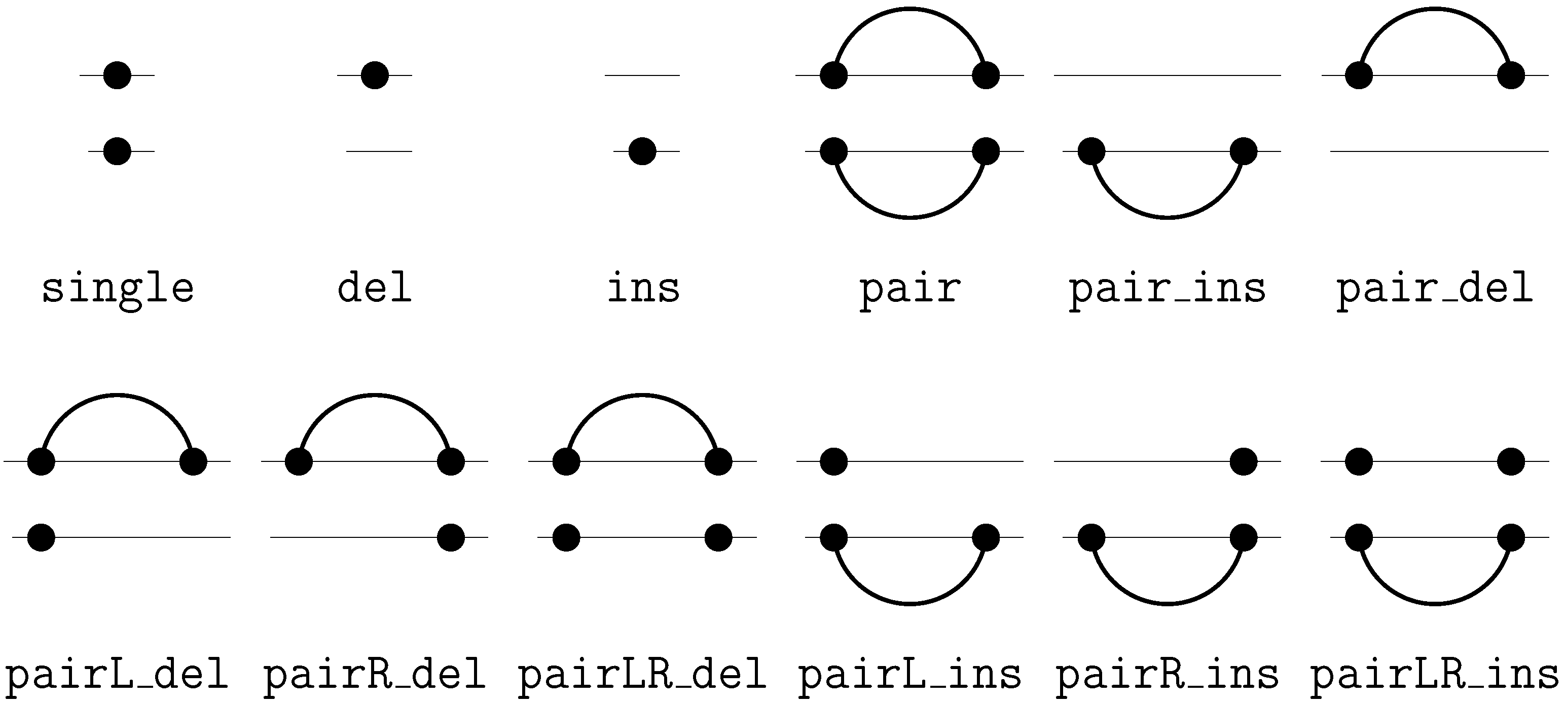
• Both satellite signatures are F.
• The core signature contains a single sort, the constant operator symbol $\mathtt{mty}$, the alphabet of the satellite signatures (if any) as nullary operators, and $2n$ operators: ${\mathtt{op}}_1^1,{\mathtt{op}}_1^2,\cdots ,{\mathtt{op}}_n^1,{\mathtt{op}}_n^2$. The arity of ${\mathtt{op}}_i^1$ and of ${\mathtt{op}}_i^2$ is the cardinality s of $var\left({\ell }_i\right)\cup var\left(r_i\right)$.
• For each edit operation ${\ell }_i\leftrightarrow r_i$, we have two rewrite rules

  $$\begin{array}{ccccc}\hfill {\ell }_i& \leftarrow & {\mathtt{op}}_i^1\left(\overline{X}\right)& \to & r_i\hfill \\ \hfill r_i& \leftarrow & {\mathtt{op}}_i^2\left(\overline{X}\right)& \to & {\ell }_i\hfill \end{array}$$

  where $\overline{X}=var\left({\ell }_i\right)\cup var\left(r_i\right)$.
• The scoring algebra is

  $$\begin{array}{ccc}\hfill {\mathtt{op}}_i^1\left(\overline{X}\right)& =& w_i+\overline{X}\hfill \\ \hfill {\mathtt{op}}_i^2\left(\overline{X}\right)& =& w_i+\overline{X}\hfill \\ \hfill \mathtt{mty}& =& 0\hfill \\ \hfill \varphi & =& max\hfill \end{array}$$
• The grammar accepts all core terms.

Note that by construction, the rewrite rules are well-defined, since $\overline{X}$ contains both $var\left({\ell }_i\right)$ and $var\left(r_i\right)$. Also note that in the core signature, no associative operator is assumed, since we are heading for a generalization of the tree alignment rather the tree edit model.

Fact 3. The above ICORE solves the tree alignment problem defined by $\{{\ell }_i\leftrightarrow r_i\}$.

Proof. By construction, two trees s and t are related by the edit operation ${\ell }_i\leftrightarrow r_i$ applied at their root position, if and only if there is a core c term rooted by ${\mathtt{op}}_i^1$ or ${\mathtt{op}}_i^2$ such that c can be rewritten under the rule ${\ell }_i\leftarrow {\mathtt{op}}_i^1\left(\overline{X}\right)\to r_i$ or $r_i\leftarrow {\mathtt{op}}_i^2\left(\overline{X}\right)\to {\ell }_i$. This argument applies recursively to the other positions in the subtrees of s and t. ☐

The simplest case of a generalized tree alignment problem is the classical one, using the atomic edit model. So our first example is an old friend:

Example 19. The ICORE TreeAlign for the alignment of trees is generated according to Definition 6 from the edit operations

$$\begin{array}{ccc}\hfill a\left(X\right)& \leftrightarrow & b\left(X\right)\hfill \\ \hfill a\left(X\right)& \leftrightarrow & X\hfill \\ \hfill X\sim Y& \leftrightarrow & X\sim Y\hfill \end{array}$$

where ${\mathtt{op}}_1^1={\mathtt{op}}_1^2=\mathtt{rep}$ (the ${\mathtt{op}}_1^2$ case is redundant because it produces the same rule as ${\mathtt{op}}_1^1$ under exchanging a and b), ${\mathtt{op}}_2^1=\mathtt{del}$, ${\mathtt{op}}_2^2=\mathtt{ins}$, and ${\mathtt{op}}_3^1={\mathtt{op}}_3^2=\sim$ (the second case is redundant because of rule symmetry).  □

Now let us move towards a non-trivial application the generalized tree alignment model. In Section 6.4, we have approached the problem of RNA structural alignment using structure-annotated sequences. Since the structures are already known when we assume structure annotated sequences as our inputs, we could as well represent the structures directly as trees (which also include the sequence information at their leaves). For our example, we use the tree representation underlying the tool RNAforester [39]. There, the nodes labeled P indicate hydrogen bonds between base pairs: $P(\mathtt{G},\mathtt{A},\mathtt{U},\mathtt{C})$ indicates that bases $\mathtt{G}$ and $\mathtt{C}$ form a hydrogen-bonded base pair, while $\mathtt{A},\mathtt{U}$ constitute the hairpin loop. Figure 12 shows an example. Therefore, the right- and leftmost sibling of a P-node must always be a base, and not another P-node. The chosen representation is captured by the following satellite signature:

Satellite signature $RST$ with

alphabet $\{\mathtt{A},\mathtt{C},\mathtt{G},\mathtt{U}\}$

operators

$$\begin{array}{cccccc}\hfill P& :& \hfill Rst& \to & Rst\hfill & --\text{must have a subforest of at least two bases}\hfill \\ \hfill \sim & :& \hfill Rst\times Rst& \to & Rst\hfill & --\text{subforest concatenation}\hfill \\ \hfill \epsilon & :& & \to & Rst\hfill & --\text{empty subforest}\hfill \end{array}$$

Figure 12. Structure representation where a P-node indicates a base pair bond between its left- and rightmost child, while the other subtrees represent structures enclosed by this base pair. In this representation, the left- or rightmost child of a P-node can never be another P-node, while the other children can.

Figure 12. Structure representation where a P-node indicates a base pair bond between its left- and rightmost child, while the other subtrees represent structures enclosed by this base pair. In this representation, the left- or rightmost child of a P-node can never be another P-node, while the other children can.

Alignments of RST trees under the atomic edit model clutter the search space with candidates that have no reasonable interpretation. For example, they allow to align a P node to a base node, or insert a P node without the two bases that make the bond. Such aligments are meaningless in this context. Replacement of P by an a must be avoided, and overall, $P(a,...,b)$ should be treated as a unit, and so on. With generalized edit operations, we can define exactly the meaningful edit operations in this scenario:

$$\begin{array}{ccccc}\hfill a& \leftrightarrow & b\hfill & & --\text{base match}\hfill \\ \hfill a& \leftrightarrow & \epsilon \hfill & & --\text{base indel}\hfill \\ \hfill P(a\sim X\sim b)& \leftrightarrow & P(c\sim X\sim d)\hfill & & --\text{base pair match}\hfill \\ \hfill P(a\sim X\sim b)& \leftrightarrow & c\sim X\sim d\hfill & & --\text{bond indel}\hfill \\ \hfill P(a\sim X\sim b)& \leftrightarrow & X\hfill & & --\text{base pair indel}\hfill \\ \hfill P(a\sim X\sim b)& \leftrightarrow & c\sim X\hfill & & --\text{paired base loss\_intro right}\hfill \\ \hfill P(a\sim X\sim b)& \leftrightarrow & X\sim d\hfill & & --\text{pair base loss\_intro left}\hfill \\ \hfill X\sim Y& \leftrightarrow & X\sim Y\hfill & & --\text{no change}\hfill \end{array}$$

for $a,b,c,d\in \mathcal{R}$ where applicable. These general edit operations ensure that editing always leads from a legal RNA structure representation to another. To create the ICORE according to Definition 6 for tree alignments under this edit model, we can almost re-use the core signature STRAL of Subsection 6.4. The overall representation has changed a bit, as we have gone from sequences to trees. This also affects the structure of their alignments. With STRAL, a base match also contains a sub-alignment of the sub-sequences following the matched bases. With RST trees, all bases reside on leaves of the trees, and sub-alignments are connected by forest concatenation instead. We design our new core signature STRAL2 following STRAL, keeping the names for analog operations, but adjusting the types. The edit operations for base match and base pair match are symmetric, and in STRAL2, they give rise to a single operator each: $\mathtt{b}\_\mathtt{match}$ and $\mathtt{pair}$. The “no change” rule is also symmmtric and gives rise to a single operator called ∼. The resulting ICORE RNATreeAli is shown on page 127.

While RNATreeAli only reformulates StructAli based on a tree representation, we can use the more general concept of tree edit operations to enrich our edit model by specific cases of interest. We give one more example.

Example 20. The iron response element is a regulatory structural motif in the ferritin pathway. It consists of a `C’-bulge, a single cytosine nucleotide that emanates from a base-paired helix. The bulge can be located upstream or downstream of the helix turn, as depicted below:

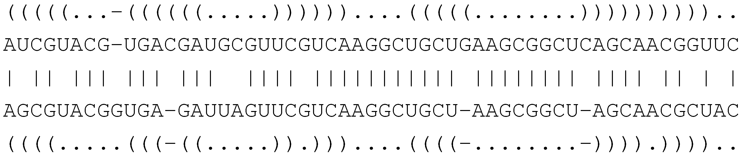
ACGCAGUGGACACUCGU            ACGAGUGGACACUCCGU

(((.(((....))))))            ((((((....))).)))

An meaningful tree alignment should probably choose indels for both ‘C’-bulges, and match the rest of the structures, as in

ACGCAGUGGACACU-CGU

(((.(((....)))-)))

(((-(((....))).)))

ACG-AGUGGACACUCCGU

The penalty of two indels can make this alignment submerged in the suboptimal candidate space. Better results can be expected with an additional edit operation such as

$$\begin{array}{ccc}\hfill P(a\sim \mathtt{C}\sim P(b\sim X\sim d)\sim e)& \leftrightarrow & P(a\sim P(b\sim X\sim d)\sim \mathtt{C}\sim e)\hfill \end{array}$$

Note that this edit operation only applies if the bulged-out nucleotide is a cytosine (C). We want this rule, because biologically, it does not matter whether the bulge is upstream or downstream of the hairpin loop. Having captured it by an edit operation, we can weight this situation as highly as a perfect match. In fact, we may even assign a bonus score to this edit operation, because where present, this situation provides evolutionary evidence for a conserved structural feature in the presence of sequence variation.  □

The tree alignment problem, in the generality as formulated here, has not been studied in the literature. For specific sets of edit operations, used for example with RNA structure, implementations are known. Overall, however, this model is an open implementation challenge. The generalized tree aligment is the most general problem we have considerd in this exposition of the ICORE framework, and hence, the solution of this problem is a central issue for the implementation of the ICORE framework as a whole. Some aspects of this challenge will be discussed in Section 10.2.

8. Evaluation Algebras and Their Products

Up to this point, we were mainly concerned with modeling the search spaces for a variety of optimization problems. Our focus was on signatures, rewrite rules and grammars. The evaluation algebras we gave were simple, or even omitted. Where shown, they were examples of one kind of scoring that could underlie our desired objective. This is fine as long as we think of each ICORE using one particular algebra. In real applications, one is much more likely to work with combinations of several algebras, called algebra products. Products do not formally extend the power of our approach, as each product could also be hand-coded as a single algebra. The gain in terms of programming productivity here comes from the fact that we can create more refined analyses from simpler ones without changing tried-and-tested code.

In algebraic dynamic programming, all scoring aspects are captured in the algebra. They are independent of the grammar and the rewrite rules. Consequently, Bellman’s Principle can be established looking at the algebra only. This, by itself, is an advantage, because we can separately experiment with either algebra, tree grammar, or rewrite system as our modeling ideas evolve.

The second benefit of such perfect separation of search space and evaluation is that one can define high-level “product” operations on two algebras over the same signature. $\mathcal{G}(A*B,x)$ does an analysis based on A and B, depending on the precise definition of “*”. And since $A*B$ is just another algebra, we can build $(A*B)*C$, $(A*B)*(C*D)$ and so on. Thus, we can build up sophisticated scoring schemes from simpler ones with a single keystroke, and if our framework understands and implements the product operation, this requires no code modification on our side. Three such products were defined with classical ADP [42], a Cartesian, a lexicographic, and an interleaved product. Let us recall the definition of the most versatile one.

Definition 7. Let A, B be two algebras over a signature Σ. The lexicographic product $A*B$ is an evaluation algebra over Σ which evaluates each candidate t according to $(A*B)\left(t\right)=\left(A\right(t),B(t\left)\right)$ and applies the objective function

$$\begin{array}{cc}\hfill {\varphi }_{A*B}& [(a_1,b_1),\dots ,(a_m,b_m)]=[(l,r)\mid \hfill \\ & l\in \mathrm{set}\left({\varphi }_A[a_1,\dots ,a_m]\right),\hfill \\ & r\in {\varphi }_B[r^{\prime }\mid (l^{\prime },r^{\prime })\leftarrow [(a_1,b_1),\dots ,(a_m,b_m)],l^{\prime }=l]]\hfill \end{array}$$

(17)

where $\mathrm{set}$ reduces a multiset of values to a set.  □

Said in words: The search space is evaluated according to A, and the candidates resulting from this are re-evaluated according to B. When both algebras optimize under some ordering, their product performs optimization under the lexicographic combination of the two orderings; this motivates the name of the product. But the lexicographic product is useful also in cases where some of the algebras involved do not perform optimization.

To demonstrate the versatility of this product operation,, let A and B be two scoring algebras with different optimization objectives, C a “counting” algebra which assigns to each candidate a score of 1, and ϕ sums up the scores, D an algebra that computes a classification attribute from each candidate, and P an algebra that computes a print representation from a candidate. For D and P, ϕ is the identity, i.e., no optimization is performed. For example, $\mathcal{G}(P,x)$ would simply print all candidates in the search space of x. We show in Table 2 some analyses which can be achieved with $A,B,C,D$, and P in lexicographic products. All three product operations mentioned above have been implemented for classical algebraic dynamic programming in the Bellman’s GAP system [16,42], where they have proved useful in real-world applications; they should work with ICOREs just as well.

Table 2. Various uses of the lexicographic product, as given in Definition 7, with different kinds of algebras.

Algebra Product	Computes	Remark
A	optimal score under A
B	optimal score under B
$A*B$	optimal under lexicographic
	order on $(A\times B)$
C	size of candidate space	avoids exponential explosion!
$A*C$	score and number of co-optimal
	candidates under A
$A*B*C$	score and number of co-optimal
	candidates under ($A\times B$)
P	representation of all candidates	complete enumeration!
$A*P$, $A*B*P$	score and representation	also known as
	of co-optimal candidates	co-optimal backtrace
D	classification attributes	all candidates’ attributes
	of all candidates	(useless by itself)
$D*A$, $D*A*B$	optimal score within each	“classified” DP
	class as assigned by D
$D*A*P$, $D*A*B*P$	opt. score and candidate
	for each class
$D*C$	size of each class
	(number of candidates)

Table 2. Various uses of the lexicographic product, as given in Definition 7, with different kinds of algebras.

Algebra Product	Computes	Remark
A	optimal score under A
B	optimal score under B
$A*B$	optimal under lexicographic
	order on $(A\times B)$
C	size of candidate space	avoids exponential explosion!
$A*C$	score and number of co-optimal
	candidates under A
$A*B*C$	score and number of co-optimal
	candidates under ($A\times B$)
P	representation of all candidates	complete enumeration!
$A*P$, $A*B*P$	score and representation	also known as
	of co-optimal candidates	co-optimal backtrace
D	classification attributes	all candidates’ attributes
	of all candidates	(useless by itself)
$D*A$, $D*A*B$	optimal score within each	“classified” DP
	class as assigned by D
$D*A*P$, $D*A*B*P$	opt. score and candidate
	for each class
$D*C$	size of each class
	(number of candidates)

9. Relation with Other Formal Models

This section covers the relation of ICOREs to earlier approaches, and also justifies some of our decisions in defining ICOREs. We first review Algebraic Dynamic Programming (ADP) [13], Searls’ transducers [43] and Lefevbre’s S-attribute grammars [11]. We then discuss why ICOREs are not Turing complete, and why grammars are mandatory in ICORE definition to guarantee the full expressiveness of the model.

9.1. “Classical” ADP Algorithms Seen as ICOREs

ICOREs build upon and extend the framework of ADP. Up to this point, ADP has been formulated solely for problems where the inputs are sequences [13,42], whereas ICOREs can also handle ordered trees. But the transition from ADP to ICOREs is deeper than just a change of the input data type. In ADP, the tree grammar is responsible for defining the search space and relating its candidates to the input sequence(s). A process called yield parsing serves as the underlying machinery for the implementation of ADP programs. With ICOREs, the tree grammar takes only responsibility for defining the search space over all problem instances, while the relation to a concrete problem instance is established by the inverse coupled rewrite relation. This brings more expressive power–but a direct implementation in the style of a yield parser is no longer at hand. What remains common to both ADP and ICOREs is the evaluation of the search space via scoring algebras.

Claiming that ICOREs subsume ADP in a mathematically strict sense, we should indicate how an ADP algorithm is re-coded as an ICORE. Formally, ADP uses input sequences over alphabets, tree grammars and signatures, but no rewrite rules. Let Σ be a signature over alphabet $\mathcal{A}$. A tree grammar $\mathcal{G}$ over Σ specifies a language of trees, $L\left(\mathcal{G}\right)\subseteq T_{\Sigma }$ as usual. The yield string $y\left(t\right)$ of a tree $t\in T_{\Sigma }$ is the string of its leaf symbols from $\mathcal{A}$, in their left-to-right order. Let $\mathcal{E}$ be a Σ-algebra with objective function ϕ, and let $x\in {\mathcal{A}}^{*}$ be our input sequence. An ADP problem instance is defined by $\mathcal{G}$, $\mathcal{E}$, and x. Its solution is

$$\begin{array}{c}\hfill \mathcal{G}(\mathcal{E},x):=\varphi \left[\mathcal{E}\right(t\left)\right|t\in L\left(\mathcal{G}\right),y\left(t\right)=x]\end{array}$$

(18)

where square brackets denote multisets. Another way to express the above definition would be (where ∘ denotes function composition and $\mathcal{E}(...)$ evaluates to a multiset.)

$$\begin{array}{c}\hfill \mathcal{G}(\mathcal{E},x)=(\varphi \circ \mathcal{E})(y^{-1}\left(x\right)\cap L\left(\mathcal{G}\right))\end{array}$$

(19)

The process of computing $y^{-1}\left(x\right)\cap L\left(\mathcal{G}\right)$ is called yield parsing, and a top-down or bottom-up yield parser is the basic engine behind ADP implementations.

Such an ADP specification given by $\Sigma ,\mathcal{G}$ and $\mathcal{E}$ is converted into an equivalent ICORE as follows:

The ICORE schematic_ADPintroduces a satellite signature $SEQ$ for the input sequence, uses Σ as the core signature, and retains the tree grammar. In the rewrite rules of form, $x_i$ and $x_j$ are different variables even when $X_i$ and $X_j$ are the same non-terminal symbol, and the righthand side produces a portion of the yield string of $t(x_1,...,x_k)$. Remember that t must not be a single variable, as term rewrite rules of the form $x\to \dots$ are not allowed. Therefore, chain productions $X\to Y$ in $\mathcal{G}$ cannot give rise to rewrite rules, and this is why we need to retain $\mathcal{G}$ as a grammar in the ICORE rather than simply replacing it with $T_{\Sigma }$. By construction, the rules in this ICORE rewrite a core term $t\in L\left(\mathcal{G}\right)$ to its yield string $y\left(t\right)\in {\mathcal{A}}^{*}$. Constructing the inverse of this particular relation is yield parsing. Hence, the same set of core terms is evaluated in Equation (19) and in the ICORE schematic_ADP by virtue of Definition 4).

The above construction was given for a n ADP program with single input. For several input sequences, ADP uses a multi-track tree grammar. In this case, each track of the grammar gives rise to a component in the coupled rewrite rules. This proves the equivalence of the search spaces in the ADP and the ICORE problem specification.

On the side of evaluation algebras, there is no difference between ICOREs and ADP. In particular, the product operations $*,\otimes$, and × on algebras [42], as sketched for * in Section 8, carry over to ICOREs and provide the programming convenience already experienced with ADP.

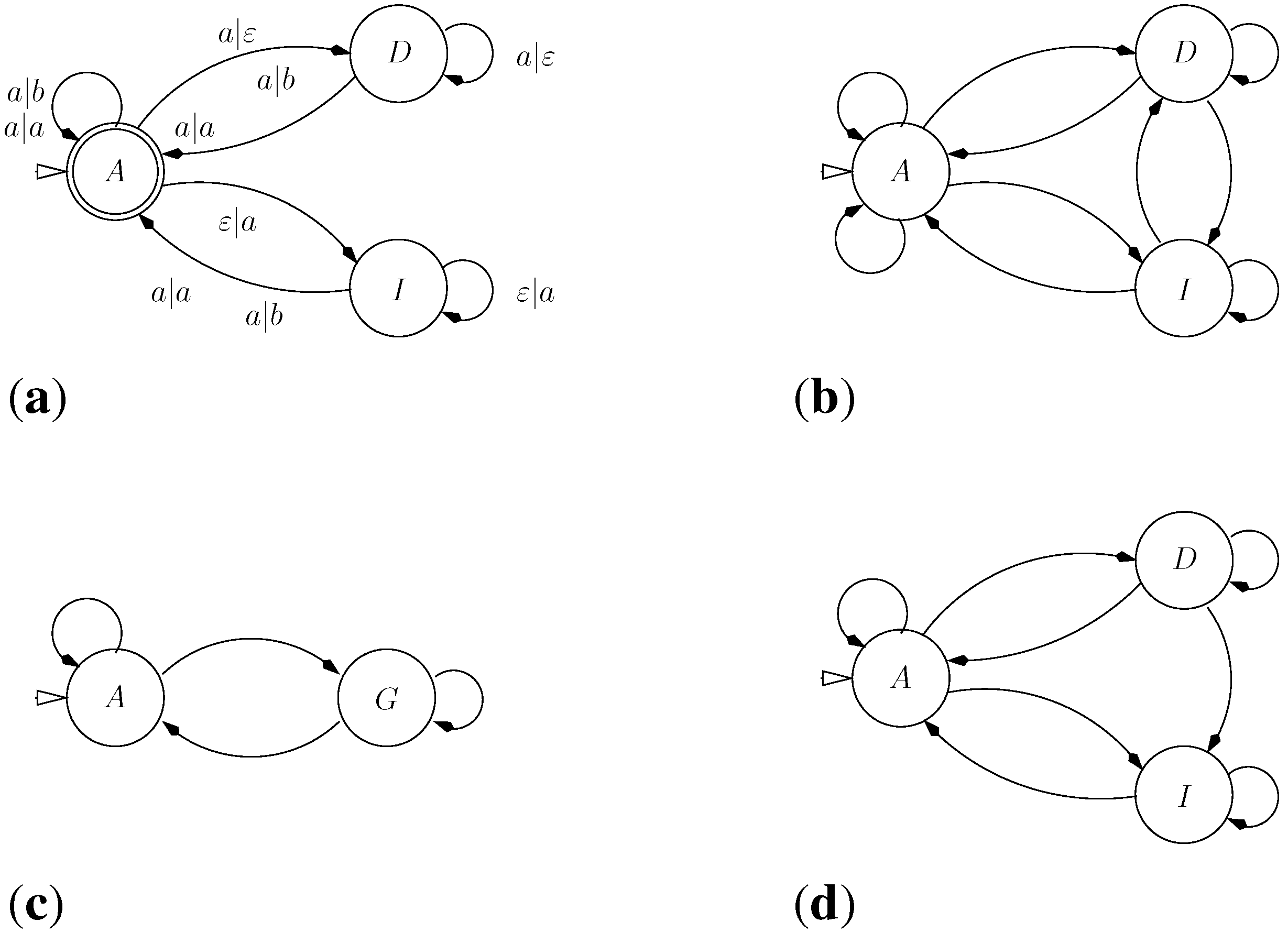
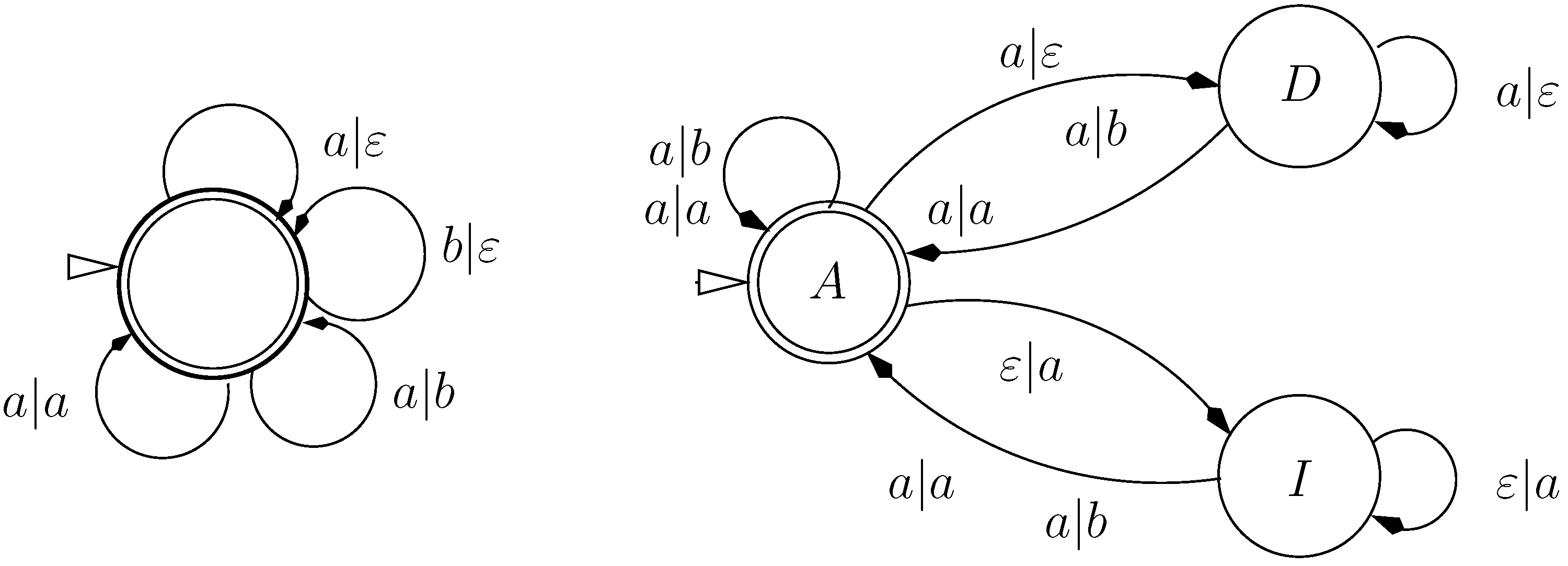
9.2. Letter Transducers Seen as ICOREs

In Section 1.3, we mentioned the work of Searls, who proposed a general formalization of edit distance based on a class of transducers, called editors [43]. We show here that the general mechanism of editors, and more generally of any transducer, can be embedded in the framework of ICOREs. Following [43], let $\mathcal{R}$ be a weighted finite transducer given by

• a finite set of states Q
• a set of initial states, $I\subseteq Q$
• an input alphabet ${\Sigma }_1$
• an output alphabet ${\Sigma }_2$ and
• a weighted transition relation $\delta \subseteq Q\times Q\times ({\Sigma }_1\cup \left\{\epsilon \right\})\times ({\Sigma }_2\cup \left\{\epsilon \right\})\times IR$

Figure 13. Transducers for edit string distance: simple edit distance (left) and edit distance with affine gap weights (right). In Searls’ terminology, these transducers are called editors.

Figure 13. Transducers for edit string distance: simple edit distance (left) and edit distance with affine gap weights (right). In Searls’ terminology, these transducers are called editors.

Such a transducer edits sequence u into sequence v, rewriting each character in u exactly once. Each step makes a transition under δ, and the transition weights sum up to the weight of a derivation. A derivation of minimal weight designates an optimal editing of u into v. Figure 12 shows two tranducer examples.

We can build a corresponding ICORE of dimension 2 in the following way.

We have the following property: The string v in ${\Sigma }_2^{*}$ is an output for u in ${\Sigma }_1^{*}$ for $\mathcal{R}$ visitingthe list of states $p_1,\dots ,p_n$ and weight α if, and only if, there exists a core term t, character symbols $u_1,\cdots ,u_n\in ({\Sigma }_1\cup \left\{\epsilon \right\})$, character symbols $v_1,\cdots ,v_n\in ({\Sigma }_2\cup \left\{\epsilon \right\})$ such that

• $u=u_1\sim \cdots \sim u_n$, $v=v_1\sim \cdots \sim v_n$
• $t={\mathtt{op}}_{p_1}^{p_2}(u_1{v}_1,{\mathtt{op}}_{p_2}^{p_3}(u_2,v_2,\cdots {\mathtt{op}}_{p_{n-1}}^{p_n}(u_n,v_n,\mathtt{mty})\cdots )$
• t belongs to the language of the grammar $\mathcal{G}$
• $u{\leftarrow }^{*}t{\to }^{*}v$
• t evaluates to α

Example 21. (String edit distance) Searls and Murphy showed that the (weighted) edit distance of two strings can be computed by a (weighted) single-state transducer and that edit distance with affine gap weights requires three states (see Figure 12). It is straightforward to verify that when we apply to them the above construction, we arrive at the ICOREs EditDistance and Affine of Section 4.2 and Section 5.1, respectively.  □

9.3. Multi-Tape S-Attribute Grammars

Lefebvre observed that Searls’ transducers could be described by regular grammars generating two strings [11]. He suggested to use context-free grammars with several input “tapes” for comparative structure analysis, named multi-tape S-attribute grammars (MTSAGs). Evaluation of structures was modeled by attribute grammars [12]. Their simplest form uses only synthesized attributes, which permits attribute evaluation by a pure bottom-up strategy as employed in dynamic programming. Lefebvre suggested a special parser for MTSAGs, which better adapts to the actual complexity of a grammar than the CYK algorithm. He modeled SCFGs by 1-tape MTSAGs, the Sankoff algorithm by a 2-tape MTSAG, as well as a restricted class of pseudoknots by a MTSAG that reads the same sequence on two tapes. Although full of innovative ideas, this line of work was not continued by others, possibly because of the very specialised parsing technlogy. MTSAGs can be emulated by ICOREs where (1) all inputs must be strings; (2) a “flat” tree grammar is used where righthand sides have tree height 1 or 0, and (3) the core signature holds one function per grammar rule for computing the synthesized attribute. Point (3) gives up the independence of search space construction and evaluation, and we would loose the flexible combination of grammars and algebras over the same signature.

9.4. Relations between Turing Machines and ICOREs

We have shown in Fact 1 that ICOREs can not apply to undecidable problems. Still, it is well-known that, as a formalism, rewrite systems are Turing-complete. In [44], Huet and Lankford simulate Turing machines by term rewriting systems such that a given machine halts with the same result if, and only if, the corresponding term rewrite system terminates for all terms. We give here a tentative adaptation of this encoding within the ICORE framework, to highlight the frontier between decidability and undecidability. We will see that we will be confronted to the imposed restriction that no part of a term is rewritten twice in an ICORE.

Consider a one-tape Turing machine with tape alphabet $\mathcal{A}$, set of states Q, and transition function δ. We introduce a binary operator symbol $\mathtt{head}$ that takes as parameters the current state of the machine and a symbol read from a cell of the tape. We represent the configuration of a Turing machine as a term

$$a_1\sim ....\sim a_{i-1}\sim \mathtt{head}(q,a_i)\sim a_{i+1}\sim ...\sim a_n$$

where the finite information on the tape is $a_1\sim ....\sim a_{i-1}\sim a_i\sim a_{i+1}\sim ...\sim a_n$, the machine is in state q, and the read-write head is on cell i.

Since ICOREs are defined as inverse rewrite systems, the result of the Turing machine computation is the core term, and the ICORE rules run the Turing machine transitions backwards.

Note that in these rules, a and b are not variables, but are a shorthand notation for one rule per alphabet symbol, encoding the Turing machine’s transition table. So, all rules are legal rewrite rules. For example, $a^{\prime }\sim \mathtt{head}(s,b)\to \mathtt{head}(q,a)\sim b$ indicates that in state q, the tape content a under the head is changed to $a^{\prime }$, the machine enters state s, and the head moves right when you apply the inverse of this rule.

Turing is not a legal ICORE, since the operator $\mathtt{head}$ occurs on both sides of the rewrite rules. This has been explicitely banned in Definition 1: The core signature and the satellite signature should be disjoint, so that a position in a core term can be rewritten only once. So what does this example tell us ? This shows that allowing arbitrary rewrite sequences would bring us into the realm of Turing machines. While it might be possible to relax this restriction in a controlled fashion, dropping it altogether would render ICOREs Turing-complete, and we could no longer hope to achieve automated and efficient ICORE implementations via dynamic programming.

9.5. A Trade-off between Grammar and Rewrite Rules

ICOREs provide two means to define the search space for given inputs, i.e., the set of core terms that are meaningful solution candidates: (1) Given core signature C, the tree grammar G restricts the search space to $L\left(G\right)$, a subset of $T\left(C\right)$. (Many ICOREs simply use the full set $T\left(C\right)$.) (2) The rewrite rules are such that some terms in $L\left(G\right)$ cannot be rewritten, no matter what the inputs are. They are not in the reverse image of the rewrite relation, and according to Definition 4, they are not candidates. In some cases, there appears to be a trade-off between these two mechanisms. We illustrate it with the following sequence alignment problem, which is a refinement of ICORE EditDistance.

Assume we are aligning protein-coding DNA sequences. Words in the genetic code consist of three nucleotides. We therefore impose the condition that all gaps have a length divisible by 3. We sketch two ICORE variants for this problem to demonstrate the above trade-off.

The first option is to modify the rewrite rules in such a way that only core terms that are legal alignments can be reduced.

Rules

$$\begin{array}{ccc}\hfill a\sim b\sim c\sim X\leftarrow & \mathtt{del}(a,\mathtt{del}(b,\mathtt{del}(c,X)\left)\right)& \to X\hfill \end{array}$$

(20)

$$\begin{array}{ccc}\hfill X\leftarrow & \mathtt{ins}(a,\mathtt{ins}(b,\mathtt{ins}(c,X)\left)\right)& \to a\sim b\sim c\sim X\hfill \end{array}$$

(21)

This set of rules defines a partial rewrite relation. A core term with singleton deletions, such as e.g. $\mathtt{rep}(a,b,\mathtt{del}(c,\mathtt{rep}(e,f,X)\left)\right)$ cannot be rewritten at all. This is intended, as this term encodes an alignment that is not authorized in the edit scheme.

The alternative is to specify a more restrictive grammar for the core terms:

Grammar

$$\begin{array}{ccc}\hfill S^{*}& \to & \mathtt{del}(a,D_1)|\mathtt{ins}(a,I_1)\left|\mathtt{rep}(a,b,S)\right|\mathtt{mty}\hfill \\ \hfill D_1& \to & \mathtt{del}(a,D_2)\hfill \\ \hfill D_2& \to & \mathtt{del}(a,S)\hfill \\ \hfill I_1& \to & \mathtt{ins}(a,I_2)\hfill \\ \hfill I_2& \to & \mathtt{ins}(a,S)\hfill \end{array}$$

This has the same effect as the partial rewrite relation above: indels come in groups of three, and alignments where this is violated are no longer in the search space. Here we can live with the original, simpler rewrite rules such as $\mathtt{del}(a,X)\to X$ and a complete rewrite relation, because the malformed gap terms are forbidden by the grammar.

Given this trade-off, one might ask if the tree grammar is strictly necessary (aside from being convenient) for the modeling power of ICOREs.

Fact 4. Tree grammars are a necessary concept in ICOREs.

Proof. We give a specific example where the search space restriction imposed by the grammar cannot be expressed via the rewrite relation. Recall sequence alignment under the affine gap model, ICORE Affine of Section 5. We have for some $n>1$

$${\mathtt{a}}^{n+1}\leftarrow \mathtt{open}\_\mathtt{del}(a,{\left\{\mathtt{del}{(\mathtt{a},\}}^n\mathtt{mty}\left\{\right)\right\}}^n\to \epsilon$$

which implies (With a finite rewrite system, we can require that up to k nested $\mathtt{del}$ operations can only be rewritten together with a leading $\mathtt{open}\_\mathtt{del}$, but k would have to be a constant while n is arbitrary.) that

$${\mathtt{a}}^n\leftarrow {\left\{\mathtt{del}{(\mathtt{a},\}}^n\mathtt{mty}\left\{\right)\right\}}^n\to \epsilon$$

Hence, without the grammar, this mal-formed term is in the search space, and under the usual kind of scoring, it scores even better than the legal

$$\mathtt{open}\_\mathtt{del}(a,{\left\{\mathtt{del}{(\mathtt{a},\}}^{n-1}\mathtt{mty}\left\{\right)\right\}}^{n-1}$$

Therefore, the grammar is required to ban malformed alignments from the search space. ☐

We conjecture that grammars could be dropped from the ICORE framework by defining a more sophisticated rewrite relation. However, we find it better to use two simple and well known mechanisms in combination, rather than a single but more sophisticated one.

10. Conclusions

ICOREs can serve two purposes in the development of combinatorial algorithms. First, they allow to specify algorithmic problems in a concise and declarative way, such that ideas can be re-used between related problems, and problems can be analyzed, refined or combined without being hindered by implementation detail. In this paper, we have examined all these aspects, and we hope that the preceding sections have given strong evidence of this virtue. Second, ICOREs may become the starting point for painless algorithm implementation. One can boldly think of an ICORE language and compiler where such a system would generate prototype implementations or even competitive code automatically from the specifications. We conclude our study with a review of what has been achieved on the first issue, and an outline research challenges that must be mastered to achieve the second goal.

10.1. ICOREs as a Declarative Specification Framework

Application range. We have taken our reader on a tour of about 30 dynamic programming problems which arise in molecular sequence and structure analysis. These include various modes of pairwise sequence comparison, pattern matching in sequences, structure prediction from a single sequence, and consensus structure prediction from a pair of sequences. Structures are compared with a variety of tree editing models. Families of sequences and structures are encoded as HMMs or SCFGs. Dressing up classical bioinformatics algorithms systematically as ICOREs, we have also obtained some novel insight.

• In the introduction to this article, we informally stated that the Sankoff algorithm for consensus structure prediction can bee seen as running two RNA folding and one sequence alignment algorithm simultaneously. In creating the Sankoff ICORE, we literally copied twice the rules from RNAfold and imported two rules from EditDistance–this was the complete Sankoff specification.
• We feel that our description of covariance model construction in three steps, going from RNAfold via Sankoff and S2SExact to CM_r is more systematic than what we find in the literature, and in particular, it points out the role of RNAfold as a model architecture in covariance model design. One could start from a different model architecture, but then proceed in the same fashion.
• The generic covariance model S2SGeneric, the Sankoff-variant SimFold and the generalized tree edit model exemplified by RNATreeAli are new algorithmic problems and deserve further investigation in their own right.

By this tour d’horizon, we hope to have convinced our readers that ICOREs are a useful concept for algorithm design, and that their automated implementation is worth a substantial research effort.

Throughout this work, we have left open the problem of the formal expressivity of ICOREs: How can we circumscribe the limits of what can be done with ICOREs? We have shown that ICOREs are not Turing complete. This is not sufficient to give us any insight on what can be achieved conveniently with ICOREs. Clearly, if problems have no sequence or tree-structured input, our machinery does not apply. This holds for a large class of dynamic programming problems studied in operations research (see e.g., [45]) or in graph theory. (It is instructive to consider the knapsack problem, where n items with individual weight and utility are given. A knapsack of maximum utility is to be packed, the overall weight of which must not exceed W. This is an NP-complete problem which whas a pseudo-polynomial solution by a DP algrithm that runs in $O\left(nW\right)$. In one dimension, the recursion runs over a list of items, selecting only from items 1 through i in each step. This dimension is easily captured in an ICORE Knapsack, reading the lists of available items in some order and making yes/no decisions. The other dimension recurs over weights from 0 to W. This requires us to do traditional style dynamic programming within the scoring algebra, either by keeping multi-sets of partial utilities sorted by weight, or by computing for each step i a single, optimal utility vector indexed by weight. Yet another alternative would be to encode the recursion over weights in a tree grammar of size W ... In either case, we see no advantage in using the ICORE approach with this problem.)

Note that ICOREs are not restricted to polynomial time problems. The inverse rewrite image of the input is typically of exponential size. Our objective functions may compute more than a single result, and they often do. “Classified” dynamic programming [16] uses a product $A*B$ to perform optimization with respect to a scoring algebra B in a class-wise fashion, based on a classification attribute computed by algebra A. Probabilistic shape analysis of RNA sequences [46] is a practical case where the number of classes is (mildly) exponential. And it is not difficult to encode 3SAT as an ICORE, yielding an exponential-time algorithm. So the question is: What can be done conveniently and efficiently with ICOREs? Our hope and goal of future research is to show that if a class of problems over sequences or trees has a known, efficient dynamic programming solution, then we can model such problems as ICOREs.

Constraints and benefits in building ICOREs. ICOREs are based on a small number of well-understood formal concepts: Algebras, grammars, and rewrite systems. Although those concepts are likely to be familiar to any computer science graduate and have a strong intuitive appeal, we are that aware that designing an ICORE requires some discipline.

Assume Paul is a programmer, experienced in the implementation of dynamic programming algorithms in the classical, non-algebraic style. The last thing Paul would think of when facing a new problem is to design a data type to explicitly represent the candidates in the search space. Indeed, the efficiency of dynamic programming comes from the fact that candidates are not constructed explicitly. Dynamic programming only derives score values from (some) candidates, and for the optimal one(s), the backtrace constructs (only) a visualization. What is eventually printed in the output need not reflect in full detail the case analysis that has rendered this particular candidate optimal. Therefore, from the experience of Paul, there is no need for a candidate data type. In fact, when we look at present-day algorithm textbooks, such as [47,48], there is not one case where such a data type is introduced. With ICOREs, Paul will have to explicitly declare a core signature on which terms represent solution candidates. The whole problem is now split in three parts: A grammar defines the universal search space, rewrite rules define the search space of a problem instance (as the inverse rewrite image of the problem inputs), and algebras provide scoring and optimization objective. If all Paul plans to do is solving a single optimization problem under a simple scoring scheme, all this machinery must appear unnecessary and verbose. However, we hope to have demonstrated that this separation of concerns, which emerges from the core signature, has a profound and beneficial effect on how we develop specifications in more sophistcated application scenarios.

• The definition of the search space is independent of any scoring algebra. We can experiment with altermative models, we can refine rules and/or grammar, for example to eliminate mal-formed candidates from the search space (rather than tricking with $\pm \infty )$. We can test how the size of the search space is affected by design decisions, independent of scoring. We can worry about (non-)ambiguity of our problem decomposition by studying properties of the grammar.
• When it comes to evaluating candidates, we can formulate arbitrary algebras over the given signature. For each, we need to prove that it satisfies Bellman’s Principle. Fortunately, this is independent of the search space and how it is constructed.
• Rewrite systems and algebras can be combined correctly in a modular fashion, bringing to bear the software engineering principles of component re-use and ease of modification.
• Finally, as seen in Section 8, the ability to define product operations on algebras and produce refined analyses from simpler ones is also due to the perfect separation of search space and evaluation of candidates.

10.2. Research Challenges in ICORE Implementation

In this article, we have left open the question of how to produce automatically an implementation from an ICORE specification. An ICORE implementation must, first of all, bring in the dynamic programming machinery that allows us to evaluate search spaces of exponential size in polynomial time. Beyond this, it should achieve the best asymptotic time efficiency, minimize the number of dynamic programming tables required, and achieve reasonable constant runtime factors for the specific ICORE at hand. Similar work has already been carried out with the Bellman’s GAP system for Algebric Dynamic Programming [16]. This makes us optimistic about what can be achieved for ICOREs. We review some problems, pitfalls, and sketch some lines of research.

Prototyping ICOREs. ICOREs can be easily coded in a functional-logic language. In such a language, we can define some function f, specify a value y and solve equational queries such as $f\left(x\right)=y$, producing all instances of x that satisfy the query equation. We have used the functional-logic language Curry [49] to prototype the ICOREs EditDitance and TreeAlign. Of course, the standard inference machine of such a language does not know that this particular type of query can be solved in polynomial time by employing dynamic programming. It actually implements a generate-and-test strategy over a search space of exponential size. We can only align trees up to five nodes in reasonable time. Still, this is a quick way to test if a given ICORE does what it is supposed to do. Languages such as Haskell, or Dyna could also be considered as host languages [50,51].

Implementing ICOREs. Aiming at more competitive implementations, quite a few technical problems must be solved in order to efficiently implement the construction and evaluation of the inverse rewrite image of a given problem instance.

• Search space construction: Grammar and rewrite rules must be used jointly to construct the search space by an interleaved enumeration of core terms and their rewriting towards the input. This is inherently a top-down process.
• Rewriting modulo associativity: where required, this contributes an implementation challenge of its own to the above.
• Generating recurrences: Candidate evaluation by an algebra is simple, but is inherently a bottom-up process, which must be amalgamed with search space construction. This amalgamation takes the form of dynamic programming recurrences which must be generated.
• Tabulation design: In order to avoid exponential explosion due to excessive recomputation of intermediate results, tabulation is used. This involves decisions on what to tabulate, and how to efficiently map sub-problems to table entries.
• Repeat analysis: A special challenge arises from the fact that ICOREs allow for non-linear rewrite rules. A variable may be duplicated on the righthand side of a rule. Two copies of a core term naturally rewrite to identical sub-terms in a satellite, and the implementation must take care to exploit this fact.
• Table number, dimension and size: While tabulating every intermediate result would be mathematically correct and asymptotically optimal, space efficiency requires careful analysis of the number of dynamic programming tables, their dimensions and sizes.
• Product optimizations: Certain tasks are conveniently expressed as algebra products, but for competitive code, they require more efficient techniques than the generic implementation of a product algebra. Two cases in point are full backtracing (for near-optimal solutions) and stochastic sampling (based on a stochastic scoring algebra). For combinatorial optimization problems on trees, no such techniques have been reported, and an implementation of ICOREs will have to cover new ground in this respect.

Advancing theory. To ensure an ICORE is correctly implemented by dynamic programming techniques, evaluation algebras must satisfy Bellman’s Principle of Optimality. For each algebra originally written by the programmer, a proof of Bellman’s Principle remains a formal obligation. But how about algebras that are constructued from given ones by products? With a keystroke, new types of refined analyses can be composed from simpler ones. Often, Bellman’s Principle is preserved with a product algebra, but in general, this is not guaranteed! There appear to be two routes to assist the programmer in this situation. (1) One might seek for general theorems–conditions under which a product preserves Bellman’s Principle; (2) One might generate proof obligations automatically from a specified product, and hope to verify or disprove them with the help of an automated theorem prover. Both of these questions are yet to be investigated.

Towards an ICORE language. Heading towards an implementation of ICOREs, the pseudocode notation we have used here must be refined towards a concrete language design. Terseness must be balanced against beneficial redundancy in several repects.

• A purist might say that the signature declarations are actually redundant, as they can be inferred from the rewrite rules, as well as from the algebras.
• A programming language designer would argue that a certain degree of redundancy is necessary, to safeguard against user errors and allow the compiler to give helpful error messages.
• A software engineer would point to the need to work with evolving programs, e.g., to have a signature where not all operators are used in a particular rewrite system, but are already included for a planned refinement.

All in all, ICOREs pose an interesting ensemble of research challenges in programming methodology and software support for combinatorial optimization.

References

- Bellman, R.E. Dynamic Programming; Princeton University Press: Princeton, NJ, UK, 1957. [Google Scholar]
- Gusfield, D. Algorithms on Strings, Trees, and Sequences: Computer Science and Computational Biology; Cambridge University Press: Cambridge, UK, 1997. [Google Scholar]
- Needleman, S.B.; Wunsch, C.D. A general method applicable to the search for similarities in the amino acid sequence of two proteins. J. Mol. Biol. 1970, 48, 443–453. [Google Scholar] [CrossRef]
- Smith, T.F.; Waterman, M.S. Identification of common molecular subsequences. J. Mol. Biol. 1981, 147, 195–197. [Google Scholar] [CrossRef]
- Sankoff, D. Simultaneous solution of the RNA folding, alignment and protosequence problems. SIAM J. Appl. Math. 1985, 45, 810–825. [Google Scholar] [CrossRef]
- Ferch, M.; Zhang, J.; Höchsmann, M. Learning cooperative assembly with the graph representation of a state-action space. In Proceedings of the IEEE/RSJ International Conference on Intelligent Robots and Systems, EPFL lausanne, Switzerland, 30 September–4 October 2002.
- Reis, D.; Golgher, P.; Silva, A.; Laender, A. Automatic web news extraction using tree edit distance. In Proceedings of the 13th International Conference on World Wide Web, ACM, New York, NY, USA, 17–22 May, 2004; pp. 502–511.
- Searls, D.B. Investigating the linguistics of DNA and definite clause grammars. In Proceedings of the North American Conference on Logic Programming; Lusk, E., Overbecck, R., Eds.; MIT Press: Cambridge, MA, USA, 1989; pp. 189–208. [Google Scholar]
- Searls, D.B. The Computational Linguistics of Biological Sequences. In Artificial Intelligence and Molecular Biology; Hunter, L., Ed.; AAAI/MIT Press: Cambridge, MA, USA, 1993; pp. 47–120. [Google Scholar]
- Searls, D.B. Linguistic approaches to biological sequences. CABIOS 1997, 13, 333–344. [Google Scholar] [CrossRef] [PubMed]
- Lefebvre. A grammar-based unification of several alignment and folding algorithms. AAAI Intell. Syst. Mol. Biol. 1996, 4, 143–154. [Google Scholar]
- Knuth, D.E. Semantics of context free languages. Theory Comput. Syst. 1968, 2, 127–145. [Google Scholar] [CrossRef]
- Giegerich, R.; Meyer, C.; Steffen, P. A discipline of dynamic programming over sequence data. Sci. Comput. Program. 2004, 51, 215–263. [Google Scholar] [CrossRef]
- Giegerich, R.; Steffen, P. Challenges in the compilation of a domain specific language for dynamic programming. In Proceedings of the 2006 ACM Symposium on Applied Computing, Dijon, France, 23–27 April, 2006; Haddad, H., Ed.;
- Höner zu Siederdissen, C. Sneaking around concatMap: efficient combinators for dynamic programming. In Proceedings of the 17th ACM SIGPLAN International Conference on Functional Programming, Copenhagen, Denmark, 10–12 September, 2012; ACM: New York, NY, USA, 2012. ICFP ’12. pp. 215–226. [Google Scholar]
- Sauthoff, G.; Möhl, M.; Janssen, S.; Giegerich, R. Bellman’s GAP-A language and compiler for dynamic programming in sequence analysis. Bioinformatics 2013, 29, 551–560. [Google Scholar] [CrossRef] [PubMed]
- Baader, F.; Nipkow, T. Term Rewriting and All That; Cambridge University Press: Cambridge, UK, 1998. [Google Scholar]
- Ohlebusch, E. Advanced Topics in Term Rewriting; Springer: New York, NY, USA, 2002. [Google Scholar]
- Gotoh, O. An improved algorithm for matching biological sequences. J. Mol. Biol. 1982, 162, 705–708. [Google Scholar] [CrossRef]
- Durbin, R.; Eddy, S.R.; Krogh, A.; Mitchison, G. Biological Sequence Analysis: Probabilistic Models of Proteins and Nucleic Acids; Cambridge University Press: Cambridge, UK, 1998. [Google Scholar]
- Giegerich, R. Explaining and controlling ambiguity in dynamic programming. In Proceedings of the Combinatorial Pattern Matching; Springer: New York, NY, USA, 2000; pp. 46–59. [Google Scholar]
- Nussinov, R.; Pieczenik, G.; Griggs, J.; Kleitman, D. Algorithms for loop matchings. SIAM J. Appl. Math. 1978, 35, 68–82. [Google Scholar] [CrossRef]
- Baker, J.K. Trainable grammars for speech recognition. J. Acoust. Soc. Am. 1979, 65, 54–550. [Google Scholar] [CrossRef]
- Sakakibara, Y.; Brown, M.; Hughey, R.; Mian, I.; Sjölander, K.; Underwood, R.; Haussler, D. Recent Methods for RNA Modeling Using Stochastic Context-Free Grammars. In Combinatorial Pattern Matching 1994, Asilomar, CA, USA, June 5–8, 1994; pp. 289–306.
- Dowell, R.; Eddy, S. Evaluation of several lightweight stochastic context-free grammars for RNA secondary structure prediction. BMC Bioinf. 2004, 5, 71. [Google Scholar] [CrossRef] [PubMed] [Green Version]
- Jiang, T.; Lin, G.; Ma, B.; Zhang, K. A general edit distance between RNA structures. J. Comput. Biol. 2002, 9, 371–388. [Google Scholar] [CrossRef] [PubMed]
- Jiang, T.; Wang, L.; Zhang, K. Alignment of trees – An alternative to tree edit. Theor. Comput. Sci. 1995, 143, 137–148. [Google Scholar] [CrossRef]
- Macke, T.J.; Ecker, D.J.; Gutell, R.R.; Gautheret, D.; Case, D.A.; Sampath, R. RNAMotif, an RNA secondary structure definition and search algorithm. Nucleic Acids Res. 2001, 29, 4724–4735. [Google Scholar] [CrossRef] [PubMed]
- Reeder, J.; Reeder, J.; Giegerich, R. Locomotif: from graphical motif description to RNA motif search. Bioinformatics 2007, 23, i392. [Google Scholar] [CrossRef] [PubMed]
- Eddy, S.R.; Durbin, R. RNA sequence analysis using covariance models. Nucleic Acids Res. 1994, 22, 2079–2088. [Google Scholar] [CrossRef] [PubMed]
- Giegerich, R.; Höner zu Siederdissen, C. Semantics and ambiguity of stochastic RNA family models. IEEE/ACM Trans. Comput. Biol. Bioinf. 2011, 8, 499–516. [Google Scholar] [CrossRef] [PubMed]
- Gardner, P.; Daub, J.; Tate, J.; Nawrocki, E.; Kolbe, D.; Lindgreen, S.; Wilkinson, A.; Finn, R.; Griffiths-Jones, S.; Eddy, S.; et al. Rfam: Updates to the RNA families database. Nucleic Acids Res. 2009, 37, D136. [Google Scholar] [CrossRef] [PubMed]
- Rosselló, F.; Valiente, G. An algebraic view of the relation between largest common subtrees and smallest common supertrees. Theor. Comput. Sci. 2006, 362, 33–53. [Google Scholar] [CrossRef]
- Chawathe, S. Comparing hierarchical data in external memory. In Proceedings of the 25th International Conference on Very Large Data Bases, San Francisco, CA, USA; 1999; pp. 90–101. [Google Scholar]
- Touzet, H. Tree edit distance with gaps. Inf. Process. Lett. 2003, 85, 123–129. [Google Scholar] [CrossRef]
- Zhuozhi Wang, K.Z. Alignment between Two RNA Structures. In Mathematical Foundations of Computer Science; 25–29 August 2001; Budapest; pp. 690–702. [Google Scholar]
- Backofen, R.; Chen, S.; Hermelin, D.; Landau, G.M.; Roytberg, M.A.; Weimann, O.; Zhang, K. Locality and gaps in RNA comparison. J. Comput. Biol. 2007, 14, 1074–1087. [Google Scholar] [CrossRef] [PubMed]
- Jansson, J.; Hieu, N.T.; Sung, W.K. Local gapped subforest alignment and its application in finding RNA structural motifs. J. Comput. Biol. 2006, 13, 702–718. [Google Scholar] [CrossRef] [PubMed]
- Schirmer, S.; Giegerich, R. Forest Alignment with Affine Gaps and Anchors. In Combinatorial Pattern Matching; Springer: New York, NY, USA, 2011; pp. 104–117. [Google Scholar]
- Dulucq, S.; Touzet, H. Decomposition algorithms for the tree edit distance problem. J. Discrete Algorithms 2005, 3, 448–471. [Google Scholar] [CrossRef]
- Erik Demaine, Shay Mozes, B.R.; Weimann, O. An optimal decomposition algorithm for tree edit distance. ACM Trans. Algorithms 2009, 6. [Google Scholar] [CrossRef]
- Sauthoff, G.; Janssen, S.; Giegerich, R. Bellman’s GAP: A declarative language for dynamic programming. In Proceedings of the 13th International ACM SIGPLAN Symposium on Principles and Practices of Declarative Programming, Odense, Denmark, July 20–22, 2011; ACM: New York, NY, USA, 2011. PPDP ’11. pp. 29–40. [Google Scholar]
- Searls, D.B.; Murphy, K.P. Automata-theoretic models of mutation and alignment. In Proceedings of the ISMB, 1995; Rawlings, C.J., Clark, D.A., Altman, R.B., Hunter, L., Lengauer, T., Wodak, S.J., Eds.; pp. 341–349.
- Huet, G.; Lankford, D. On theUniform Halting Problem for Term Rewriting Systems. Technical Report, Rapport Laboria 283, IRIA. 1978. [Google Scholar]
- Powell, W.B. Approximate Dynamic Programming: Solving the Curses of Dimensionality; Wiley-Interscience: New York, NY, USA, 2007. [Google Scholar]
- Voß, B.; Giegerich, R.; Rehmsmeier, M. Complete probabilistic analysis of RNA shapes. BMC Biol. 2006, 4, 5. [Google Scholar] [CrossRef] [PubMed]
- Sedgewick, R. Algorithms; Addison-Wesley: Reading, MA, USA, 2002. [Google Scholar]
- Cormen, T.; Leiserson, C.; Rivest, R. Introduction to Algorithms; MIT Press: Cambridge, MA, USA, 1990. [Google Scholar]
- Braßel, B.; Hanus, M.; Peemöller, B.; Reck, F. KiCS2: A new compiler from curry to haskell. In Proceedings of the 20th International Workshop on Functional and (Constraint) Logic Programming; Springer: New York, NY, USA, 2011; pp. 1–18. [Google Scholar]
- Thompson, S. Haskell: The Craft of Functional Programming; Addison Wesley: Boston, MA, USA, 2011. [Google Scholar]
- Eisner, J.; Filardo, N.W. Dyna: Extending Datalog for modern AI. Datalog 2.0; Furche, T., Gottlob, G., Grasso, G., de Moor, O., Sellers, A., Eds.; Springer: New York, NY, USA, 2011. [Google Scholar]
© 2014 by the authors; licensee MDPI, Basel, Switzerland. This article is an open access article distributed under the terms and conditions of the Creative Commons Attribution license (http://creativecommons.org/licenses/by/3.0/).
Share and Cite
Giegerich, R.; Touzet, H. Modeling Dynamic Programming Problems over Sequences and Trees with Inverse Coupled Rewrite Systems. Algorithms 2014, 7, 62-144. https://doi.org/10.3390/a7010062
Giegerich R, Touzet H. Modeling Dynamic Programming Problems over Sequences and Trees with Inverse Coupled Rewrite Systems. Algorithms. 2014; 7(1):62-144. https://doi.org/10.3390/a7010062
Chicago/Turabian StyleGiegerich, Robert, and H´el'ene Touzet. 2014. "Modeling Dynamic Programming Problems over Sequences and Trees with Inverse Coupled Rewrite Systems" Algorithms 7, no. 1: 62-144. https://doi.org/10.3390/a7010062