A Faster Quick Search Algorithm

1
Faculty of Software, Fujian Normal University, Fuzhou 350108, China
2
Lane Department of Computer Science and Electrical Engineering, West Virginia University, Morgantown, WV 26506, USA
*
Author to whom correspondence should be addressed.
Algorithms 2014, 7(2), 253-275; https://doi.org/10.3390/a7020253
Submission received: 25 April 2014
/
Revised: 30 May 2014
/
Accepted: 4 June 2014
/
Published: 23 June 2014
Abstract
:We present the FQS (faster quick search) algorithm, an improved variation of the quick search algorithm. The quick search (QS) exact pattern matching algorithm and its variants are among the fastest practical matching algorithms today. The FQS algorithm computes a statistically expected shift value, which allows maximal shifts and a smaller number of comparisons between the pattern and the text. Compared to the state-of-the-art QS variants of exact pattern matching algorithms, the proposed FQS algorithm is the fastest when , where is the alphabet size. FQS also has a competitive running time when . Running on three practical text files, E. coli (), Bible () and World192 (), FQS resulted in the best performance in practice. Our FQS algorithm will have important applications in the domain of genomic database searching, involving DNA or RNA sequence databases with four symbols or protein databases with .
1. Introduction
Given a text of length n and a pattern of length m over an alphabet, Σ, the exact string matching problem is to find all occurrences of pattern P in the text, T. In general, . The exact string matching problem is an important and well-studied subject [1,2]. Three popular exact matching algorithms with linear time complexity are the Knuth–Morris–Pratt (KMP) algorithm [3], the Karp–Rabin (KR) algorithm [4] and the Boyer–Moore (BM) algorithm [5]. Like KMP, the BM algorithm matches the pattern and the text by skipping characters that are not likely to result in exact matching with the pattern. Unlike the other methods, it compares the strings from right to left of the pattern. These algorithms need an time for preprocessing the pattern, and search in or sometimes even sublinearly in practice. The total time will be . A different approach to pattern matching based on bitwise operations was introduced by R. Baeza-Yates and G. Gonnet [6]. Here, the pattern is represented by a binary mask. Bitwise SHIFT and AND operations that are considered as constant time are used to find the patterns. Under this framework, SHIFT and AND correspond to the pattern movement and matching, respectively. The algorithm is effective for small patterns, when the pattern length is less than a computer word (typically 32 or 64 characters), which is usual for the text searching problem. Bitwise parallelism is the basis of some recent improved algorithms for exact pattern matching. See [7,8] for examples.
Since Boyer and Moore published their famous BM algorithm in 1977 [5], many variants of the BM algorithm have been proposed [2,9]. Among these variants, Sunday’s quick search [10] is widely used because of its simplicity and efficiency.
Algorithms based on character comparisons can be classified into these three categories by the way they scan the text [9]: forward orientation, backward orientation and no specific direction. Forward orientation is comparing the text to the pattern from left to right. The KMP algorithm is in this category. See, also, Apostolico et al. [11] and Crochemore et al. [12]. Under backward orientation, we compare the text to the pattern from right to left; the BM is in this category. For the third category, some algorithms used both forward and backward comparisons at the same time, for example, quick search by Sunday, and its variants, the Franek–Jennings–Smyth (FJS) algorithm [13] and the Horspool algorithm [14]. See, also, the book by Charras and Lecroq for other similar algorithms [1]. The other strategy is to determine the preprocessing shift array according to the probability of symbol occurrences in the pattern [1,9].
The QS algorithm and its variants remain among the fastest practical exact pattern matching algorithms to date [9]. In this paper, we introduce faster quick search (FQS), an improved algorithm based on the QS exact pattern matching algorithm. The FQS algorithm computes a statistically expected shift length, which allows for maximal shifts and a smaller number of comparisons between the pattern and the text. FQS also utilizes the QS algorithm’s bad-character shift table (array) in preprocessing the pattern. Compared to the state-of-the-art algorithms of the QS variety, FQS is the fastest algorithm when and has a competitive running time when . Our FQS algorithm will have important applications in the domain of genome database searching, where the DNA (RNA) sequence databases consists of four symbols and for protein databases with .
In this work, we have focused on the QS variants of the Boyer–Moore string matching algorithm. More general discussions on exact string matching can be found in the textbooks, [2,12,15,16]. Two recent reviews related to the topic are [9,17].
This paper is organized as follows. First, we introduce the BM algorithm, the QS algorithm and its variants in Section 2. Next, we present the proposed FQS algorithm in Section 3. In Section 4, we present experimental results, including a comparison with three variants of the QS algorithm. Section 5 concludes the paper.
2. Boyer–Moore Algorithm and Its Variants
The Boyer–Moore (BM) algorithm is an efficient string searching algorithm introduced by Boyer and Moore in 1977 [5]. The BM algorithm has been the standard benchmark algorithm in the exact string matching literature since it was introduced [5]. The BM algorithm preprocesses the pattern, P, and utilizes the information gathered during the preprocessing step to skip blocks of text (rather than character by character comparisons) during matching, resulting in a faster running time than many other string algorithms. In general, the BM algorithm runs faster as the pattern length increases.
First, the BM preprocesses pattern P to construct a bad character shift array (abbreviated as ) of length , which is determined using Equation (1). Then, the BM uses the bad character rule. The bad character rule stipulates that once a mismatch occurs, the algorithm jumps to the next position, which is determined by the array without performing brute-force comparisons.
The BM also uses the good suffix rule. The BM starts the comparison between text T and pattern P from right to left. When a mismatch occurs in with and , the suffix of pattern matches text ; the suffix of pattern is called the good suffix. The algorithm calculates a good-shift array of length that determines the next jumping position using the maximum possible shift distance from the structure of the pattern. The overall shift value is then determined by choosing the longer distance between both the bad-shift and good-shift arrays. The classic quick search algorithm and our improved variant do not use the good suffix rule; hence, the corresponding good shift array equation is not presented here. Interested readers, please refer to the original paper by Boyer and Moore [5]. The original BM algorithm has a worst-case running time of and a best-case time in . It has very good performance in general, and there are simple modifications to achieve an overall worst-case time in time [18,19].
2.1. Quick Search Algorithm
The quick search(QS) algorithm introduced by Sunday [10] is a simplification of the Boyer–Moore algorithm without the good suffix rule. QS preprocesses pattern P using a modified bad_shift array (called ) of length in a time complexity of . The modified quick search bad shift array is defined as follows:
The preprocessing steps of the quick search algorithm are shown in Algorithm 1. In Algorithm 1, array is the quick search bad character shift array, which is initialized to value m from Line 1 to Line 3. Lines 4–6 implement Equation (2). For example, in the case of pattern P = “GCAGTCAG” with and . Each element in bad_shift array is initialized to eight. After executing the loop from Line 4 to Line 6, we have the bad_shift array .
| Algorithm 1 The preprocessing of the quick search algorithm. |
preQS(P,m) 1 for i ← 0 to |Σ|−1 2 qsBc[i] ← m 3 end for 4 for i ← 0 to m − 1 5 qsBc[P[i]] ← m − i 6 end for 7 return qsBC[] |
In Algorithm 1, Lines 1–3 run in steps; Lines 4–6 run in m steps. Thus, the total preprocessing time is .
Algorithm 2 shows the quick search algorithm. First, it calls the preprocessing procedure, , to compute the bad shift array. Lines 3–9 use a loop to compare the text, T, and the pattern, P. Line 4 compares and , where . When a mismatch occurs, the QS algorithm shifts to a new position as determined by the bad character in T, that is, using the corresponding shift value for the symbol, .
| Algorithm 2 The quick search algorithm. |
QS(P,m,T,n,|Σ|) 1 shift ← preQS(P,m) 2 j ← 0 3 while (j ≤ n − m) 4 Compare P[0,...,m − 1] and T[j,...,j + m − 1] 5 if all matched then do 6 output j 7 end if 8 j ← j + shift[T[j + m]] 9 end while |
The searching phase of the QS has a worst case time complexity of . In the case of each time, a shift distance is maintained as on,e and the bad character is found in the last comparison of to the corresponding text (QS starts the comparison from right to left). For example, if and , in this case, the shift distance . That is, when each bad character occurs, the shift distance is one. Additionally, the bad character is found at the last comparison of to the corresponding text place, because the QS comparison is from right to left. However, this extreme worst case is rare. Just like the BM, the QS has a very good practical performance in general [10].
2.2. Variants of the QS Algorithm
The QS algorithm was motivated by another simplification of the BM algorithm proposed earlier by Horspool in 1980 [14]. It has a better performance than the BM in the case of smaller alphabet sizes. The average number of comparisons for one character is between and [14]. It has the same preprocessing time of and the worst-case searching time of , as with the QS algorithm.
Another QS variant is the FJS algorithm, introduced by Franek, Jennings and Smyth [13] in 2007. FJS is a hybrid exact string matching algorithm that uses both the QS (i.e., Boyer–Moore) and Knuth–Moris–Pratt(KMP) algorithms. It has a preprocessing time, similar to the QS. FJS uses the KMP algorithm to ensure that, in the worst-case, its searching phase is , which is better in theory than the of BM, QS and other QS variants. As shown in [13], when the pattern length is small (less than 10 characters), FJS’s performance is slightly better than the other algorithms.
Another variation of the QS algorithm was proposed by Sheik et al. [20] and Thathoo et al. [21], by combing the QS algorithm with an initial pre-testing stage, as earlier proposed by Raita [22]. That is, after pre-computing the shift tables based on the QS algorithm, at the search phase, they introduce a pre-testing step, before full pattern matching can commence. Within a pattern matching window on the text, the last and first symbols in the pattern are first compared with their respective counterparts in the window on the text. If both tests succeed, pattern matching on the remaining symbols will then proceed as usual from right to left, using the QS algorithm. The idea is to establish some level of similarity between the pattern and the text window, before pattern matching will continue. A similar idea was used by Thathoo et al. [21], where they improved the basic approach and required a smaller number of comparisons and larger shifts on average. Experimental results in the recent comprehensive survey by Faro and Lecroq [9] showed that, indeed, the method of Thathoo et al. [21] was slightly better than the approach of Sheik et al. [20], in general. However, the FJS algorithm produced an overall better result when compared with the two methods. Thus, in our comparative analysis, we focused on FJS, HOR and QS.
3. The FQS Algorithm
Faster quick search (FQS) is an improved version of the quick search algorithm. QS calculates a shift table (array) using Equation (2). In addition to the same shift table in the QS algorithm, FQS calculates two more elements: one is the maximal expected shift position (called ); the other is a new shift table for the prefix using the QS algorithm. The expected shift (ES) is the sum of shifts when a mismatch occurs in the pattern current position. In our algorithm, the shift is calculated by the bad character rule, which shifts to right when matching the symbol of the text. In the uniform distribution of symbols, the maximal expected shift position is the left most position of the pattern that has the maximal expected shift value in all positions of the pattern. When the mismatching occurs in this position, it will have the largest shift value in the average case. Equation (3) calculates the expected shift distance for each position in pattern P. The maximal expected position, , is calculated in pattern P by using Equation (4). Finally, the algorithm identifies a maximal location, , which has the maximal expected shift position.
Before we introduce Equation (3), we first need to consider the array, . Given the current position, j, in pattern P and a symbol, , records the most recent occurrence position of symbol c. For example, given a pattern P = “GCAG”, let us examine the array. First, the size of array is the same as the alphabet size. Array is calculated by scanning pattern P from left to right. The initial value of is set to “”. After scanning , is changed to zero, and all of the other symbols of are still “” (the initial value). After scanning , is updated to one, because the second character is C; all of the other corresponding remain the same as . After , is updated to two; the other elements are unchanged. After , is updated to three, the other elements remain unchanged: and .
Now, consider Equation (3). is the sum of the shifts in the current position, j, of pattern P if the bad character rule is applied. For each position, j in P, where , is calculated by using Equation (3), which indicates the sum of shift values for each symbol, .
The maximal expected shift position () for pattern P is computed using Equation (4). is defined as the first position in pattern P where the maximal occur.
3.1. Preprocessing Phase
In the preprocessing phase, FQS needs to determine three elements: (1) The maximal expected shift position () for pattern P using Equation (4); (2) a shift table for pattern P using the QS algorithm; and (3) a shift table for , the prefix of P, using the QS algorithm. The maximal expected shift position (, from Equation (4)) is the maximal expected shift distance using the bad character rule. is calculated from pattern P in the preprocessing phase.
3.1.1. Computing the array
In the naive computation, for each symbol . The total time complexity for computing all , where , is . Needless to say, it can be improved. The can be calculated from , when . That is, the expected skip value at the current position can be calculated by utilizing the known expected skip value at the previous position. The difference between and is:
Since , then .
For each and . That is, all symbols in pattern P have the property that , except for the symbol at the current position, j. Put another way, except the current symbol in pattern P, for all of the other symbols in Σ, their current is equal to . The difference between and can be further analyzed:
Finally, we get:
3.1.2. Preprocessing algorithm
The preprocessing procedure is shown in Algorithm 3. We use an array, , of length , to keep the previous position for each symbol, c, where . Following the above analysis, we can get from (Equation (7)), where . The computation can be done in constant time for each given j.
| Algorithm 3 Get the maximal expected shift value. |
GetPos(P,m,|Σ|) 1 ES ← 0, maxES ← 0, pos ← 0 2 for (i ← 0 to Σ − 1) do 3 PrePos[i] ← − 1 /*initializing all of prepos*/ 4 end for 5 for (j ← 0 to m − 1) do 6 ES ← ES + |Σ| − (j − PrePos[P[j]]); 7 PrePos[P[j]] ← j; 8 if ES ≥ maxES then 9 maxES ← ES; 10 pos ← j; 11 end if 12 end for 13 return pos |
Algorithm 3 shows the detailed preprocessing steps to compute the maximal expected shift position () for pattern using Equation (4). In Algorithm 3, variable is the expected skip value, which is initialized to zero. In the first step of the loop in Lines 5–12, will be set to . Variable is the maximal expected shift value. Additionally, , a position in pattern P, is the location where the maximal expected shift value resides in the pattern, P.
Lines 2–4 initialize the value at each symbol to “” for the recent occurrence position array, (denoted as in Equation (3)). Lines 5–12 are a loop, which calculates each position’s expected shift value, , and determines the maximal expected value. Line 6 calculates the expected shift value, , using the incremental method, as discussed above (Equation (7)). Lines 9–12 search for the maximal expected shift value, . The algorithm finally returns the maximal expected shift position, , in Line 13. Note that this preprocessing is only performed once for the pattern, P, using time.
Recall that FQS calculates three elements in its preprocessing phase, namely: (1) the maximal expected shift position () for pattern P; (2) a shift table for pattern P using the QS algorithm; and (3) a shift table for , the pos-length prefix of P, again using the QS algorithm. From the above calculation of the maximal expected shift position (), we know that the time complexity is . For element (2) and (3), the computations are based on the QS algorithm, requiring time in and , respectively. Together, the overall preprocessing time complexity for FQS is , since .
3.2. Search Phase
In the search phase, FQS starts to compare the position in the pattern, P, which has the maximal expected shift value, rather than the rightest-most position in P, as in the QS (and the other BM variants). Algorithm 4 shows the detailed steps.
| Algorithm 4 FQS pattern matching algorithm. |
FQS(P,m,T,n,|Σ|) 1 pos ← GetPos (P,m,|Σ|) 2 next ← preQS(P,pos) 3 shift ← preQS(P,m) 4 j ← 0 5 while (j ≤ n − m) 6 while (P[pos] ≠ T[j+pos]) 7 j ← j + next[T[j + pos]] 8 if j > n − m then do 9 return 10 end if 11 end while 12 Compare P[0,...,m − 1] and T[j,...,j + m − 1] 13 if all matched then do 14 output j 15 end if 16 j ← j + shift[T[j + m]] 17 end while |
In Algorithm 4, the first three lines are the preprocessing steps. Line 1 calls Algorithm 3 to get the location, , with the maximal expected shift. Lines 2 and 3 calculate two shift tables (called and ) for the prefix and the entire pattern, P, respectively, using the same procedure as the classic QS preprocessing algorithm. Compared to the QS algorithm as shown in Algorithm 2, in the preprocessing phase, FQS adds two more lines: Lines 1 and 2. The total time complexity of the three steps is still .
FQS determines the maximal expected shift position. This maximal expected shift position has the statistical maximum shift distance. Once a mismatch is found, the algorithm jumps to a new position, which has the expected maximal shift distance. This mechanism significantly speeds up the FQS algorithm (see the section on the results).
After the preprocessing step, the searching strategy of FQS is as follows:
- Step 1: Check the symbols at maximal expected shift position , that is, compare symbols and ;
- Step 2: If there is a mismatch, shift pattern P based on the distance determined by . Go to Step 1 to continue checking position ;
- Step 3: If otherwise, compare to , the same way as in the QS algorithm. If all matched, a matching pattern is found at position j in T;
- Step 4: Whether all matched or not, shift the pattern to the right based on the value of using the classic quick search algorithm;
- Step 5: Repeat the above Steps 1–4 in a loop until text T is exhausted ().
In Algorithm 4, Lines 5–17 capture the searching phase. Compared with the QS algorithm, FQS adds Lines 6–11 in the search phase. In this phase, initially, text T is aligned with pattern P, at positions and , respectively, where . FQS first starts to compare the position of the maximal expected shift, in P, to the corresponding position, in T. If a mismatch occurs, the pattern is shifted to a position that is determined by the value, . These steps are performed in Lines 6–11. Otherwise, the FQS algorithm does the same thing as the QS algorithm by starting to compare pattern and from right to left.
3.3. Correctness and Complexity Analysis
3.3.1. Correctness Analysis
The correctness of the FQS algorithm essentially follows from the correctness of the QS algorithm. In the search phase, the FQS algorithm uses two bad character shift arrays in two steps. When comparing pattern P to text T, FQS first checks the position, in P, the expected maximal shift position, comparing it to the position, in T. If there is a mismatch, it uses the shift array, , to shift the pattern to the next right position. The shift value is at most . It will not miss any potential matching position. After the first symbol comparison ( vs. ), the remaining steps are the same as in the QS algorithm.
3.3.2. Complexity Analysis
Section 3.1 provided details on computing the expected maximal shift position and showed the time complexity of Algorithm 3 to be in . The other two preprocessing steps compute the shift arrays using the bad character rule, hence the time required for these two steps are also in according to the QS algorithm.
In the searching phase, the FQS algorithm integrates a pre-testing stage with the QS algorithm. The time complexity of one pre-test is constant, and the total time complexity is in . The worst-case time complexity for searching phase in the FQS is , and the average time complexity is . The extra space required by the FQS is in . The FQS algorithm has the same worst-case and average-case time and space requirements as the QS algorithm. As with the general BM algorithm, the worst case complexity can be improved to using the good suffix heuristic with memorization [2,19].
3.4. An Example
Here, we show a short example of the proposed algorithm, where text T = “GCATCGCAGTCAGTATACAGTAC” () and pattern P = “GCAGTCAG” (). The text and pattern are DNA sequences from the alphabet , hence .
3.4.1. Computing the Maximal Expected Shift Position () for Pattern P
For calculating the maximal expected shift value of the pattern P = “GCAGTCAG”, in Line 3 of Algorithm 3, the recent occurrence position ( array in Algorithm 3) for these four symbols are initialized to “”. Then, Algorithm 3 calculates for the pattern, P, by scanning from left to right.
When the first character is read (), is the initial value of . Line 6 sets . This is the expected shift distance for Position 0 in pattern P. In Line 7, is set to the current Position 0; this indicates that character G has appeared at least once at this time. In Lines 8–10, the maximal expected shift distance is set to .
When the second character is read (), Line 6 sets . In Line 7, is set to its current position, 1. In Line 9, the maximal expected shift distance is set to five.
When the third character is read (), Line 6 will set . In Line 7, is set to its current position, 2. In Line 9, the maximal expected shift distance is set to six.
When the fourth character is read (), the value has been changed to its previous appearing position; in this case, . Line 6 will set . In Line 7, is set to its current position, 3. In Line 9, the maximal expected shift distance is set to seven.

| j | 0 | 1 | 2 | 3 | 4 | 5 | 6 | 7 |
| G | C | A | G | T | C | A | G | |
| 3 | 5 | 6 | 7 | 6 | 6 | 6 | 6 | |
| Σ | A | C | G | T | ||||
| next | 1 | 2 | 3 | 4 | ||||
| Σ | A | C | G | T | ||||
| shift | 2 | 3 | 1 | 4 |
The remaining characters in pattern P are processed in a similar manner. The final expected shift distances for each position in pattern are 3, 5, 6, 7, 6, 6, 6, 6. The maximal expected shift position is in , which has a value of seven. Hence, we have the maximal expected shift distance in Position 3 of pattern P, that is, (see Table 1).
3.4.2. Computing the Shift Tables: and
We calculate the shift table for pattern prefix , which is denoted as with a value of . Additionally, the shift table for pattern is denoted as array, . Both the array and array are calculated using the classical QS algorithm; thus, we omit the detailed computation steps. See Table 1 for the values in the and arrays.
3.4.3. Searching Pattern P in T
After preprocessing steps, the search phase begins.
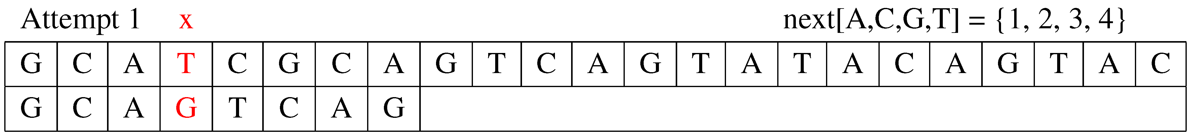
Attempt 1: The first attempt compares the pattern, P, to the text, T, from the beginning, as shown in Figure 1. Because the maximum of expected shift () is three (), the comparison starts at against the corresponding position in text . This will be the symbol, , thus leading to a mismatch. The algorithm shifts the pattern, P, to the next position with the shift distance determined by . Additionally, the value of j is updated to .
Figure 1.
The first attempt.

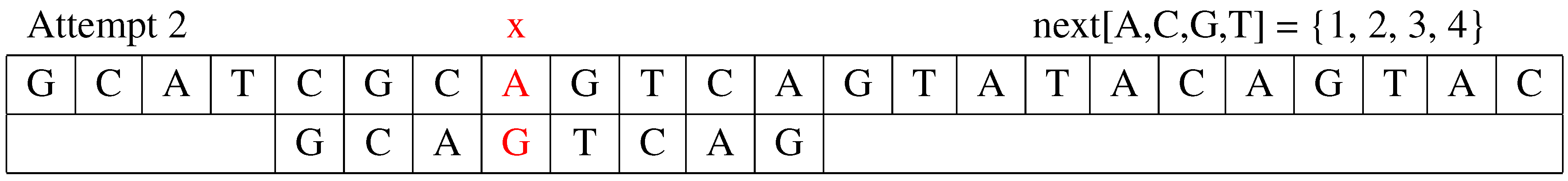
Attempt 2: The second attempt is shown in Figure 2. The algorithm still starts to compare to the corresponding position in text . It is still a mismatch. The shift distance is . The value of j is updated to .
Figure 2.
The second attempt.

Attempt 3: The third attempt is shown in Figure 3. The algorithm compares to text . The characters match. Then, the algorithm proceeds as the classic QS algorithm. After a one by one comparison, the algorithm finds an exact match here. It reports the occurrence position and determines the shift distance, j. This shift distance is determined by the classic QS algorithm .
Figure 3.
The third attempt.

Attempt 4: The fourth attempt is shown in Figure 4. Algorithm FQS compares to text . Since the symbols match, the algorithm follows the classic QS algorithm steps by comparing from right to left. The pattern’s rightmost character is G, which does not match the corresponding symbol, A in T. The algorithm determines the next shift distance , and the value of j is updated to .
Figure 4.
The forth attempt.
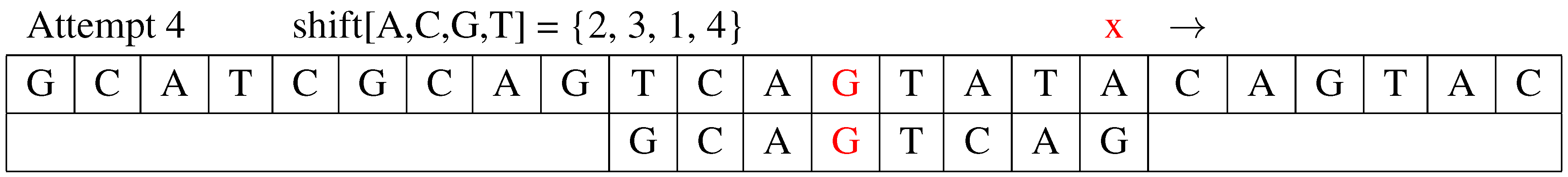
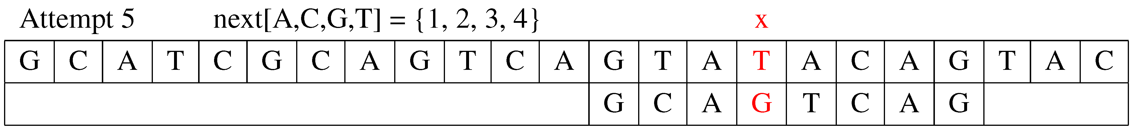
Attempt 5: The fifth attempt is shown in Figure 5. The algorithm compares to the corresponding position in text . It is a mismatch. The shift distance is determined by FQS shift value , and the value of j is updated to . For , when , text T is exhausted. The search phase stops.
Figure 5.
The fifth attempt.

4. Experimental Results
We conducted a number of experiments to compare the FQS algorithm with other state-of-the-art QS algorithms, which are known to be among the fastest in practice: FJS [13], Horspool [14] and the QS itself [10]. The implementation of FJS is provided by their authors in the paper [13]. The implementation of the other two competitive algorithms are downloaded from the website developed by Christian Charras and Thierry Lecroq (http://www-igm.univ-mlv.fr/ lecroq/string/). Their website provides the C code for a large number of exact string pattern matching algorithms, which they reviewed in [1,9]. Our implementation of the FQS algorithm is also based on the codes for the QS algorithm provided at the site.
The experiments were conducted on two sets of data: one is a set of randomized text files, the other contains three practical text files. These three practical text files, E. coli, Bible and World192, were downloaded from the Large Canterbury Corpus (http://corpus.canterbury.ac.nz/). The computing environment was a personal computer with an Intel Core2 CPU with 1.66 GHz and 8 GB of RAM working in the Ubuntu 12.04 operating system.
4.1. Randomized Text Files
We generated eight random text files with different alphabet sizes, namely, = 2, 4, 8, 16, 32, 64, 128 and 256. The size of each random text file was fixed at 100 MB. Patterns were randomly chosen from these files with 19 varying lengths: m = 10, 20, 30, 40, 50, 60, 70, 80, 90, 100, 200, 300, 400, 500, 600, 700, 800, 900 and 1,000, respectively. For a given pattern length, 50 different patterns were randomly chosen to search in each text file. The average running times were then calculated from these 50 runs.
The experimental results are shown separately for two cases: (1) the pattern length is less than or equal to 100 (); and (2) the pattern length is greater or equal to 100 (). The results show the following:
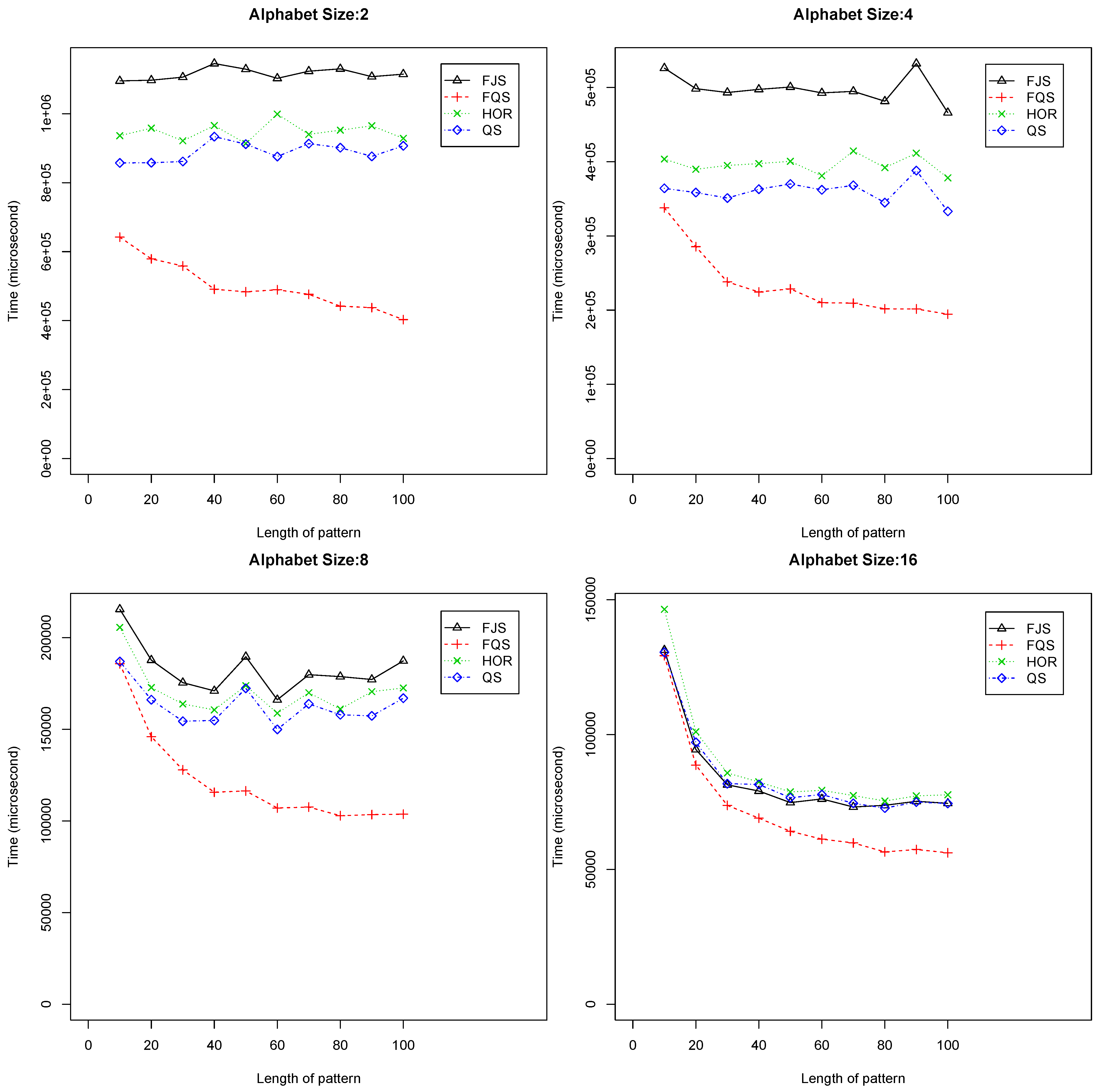
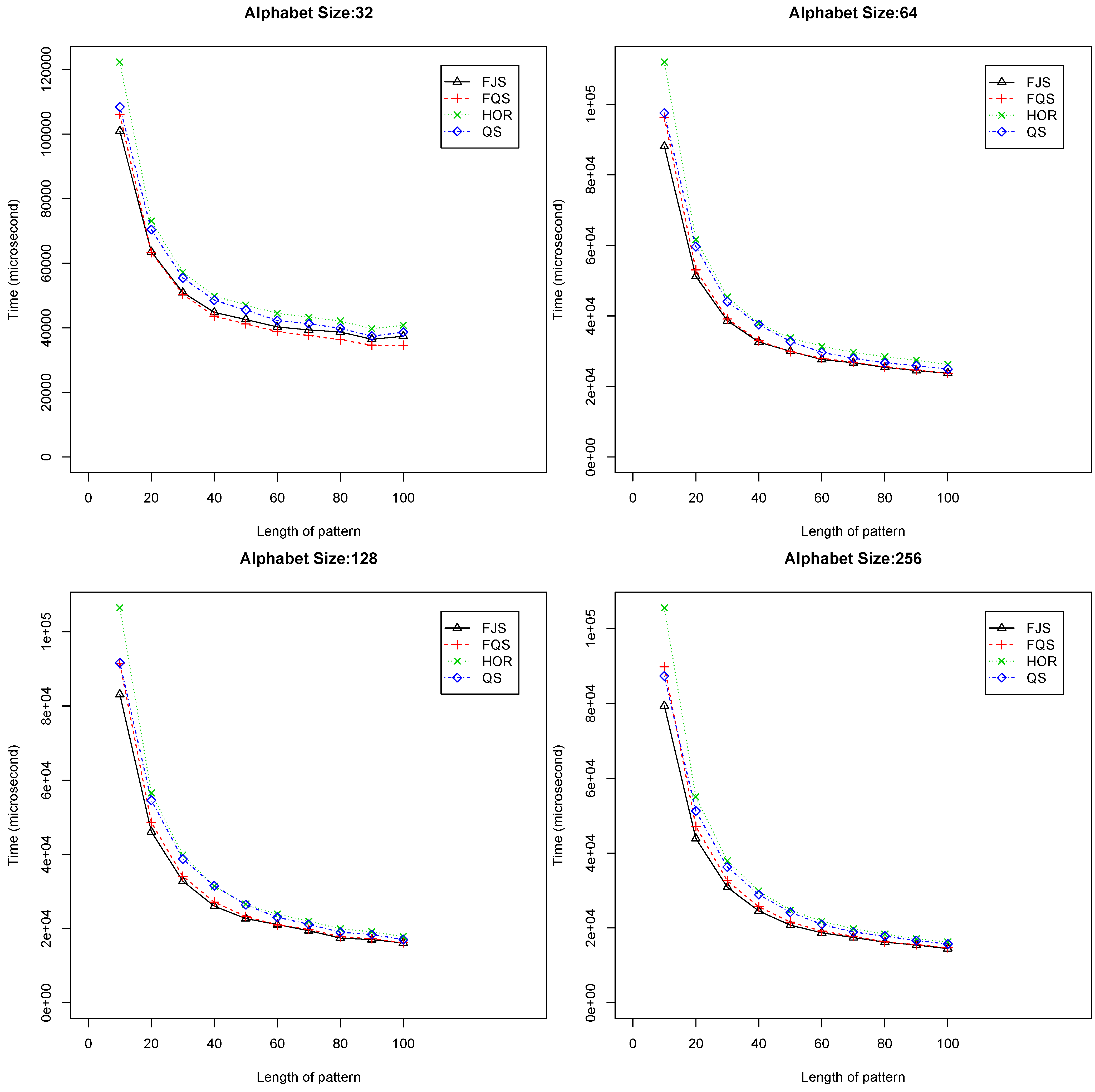
- When and , FQS is much faster than the others. Figure 6 shows the performance of the algorithms in these cases. When , the trends are similar: FQS is the fastest algorithm among the four. The QS is the second best, which is slightly better than Horspool (denoted as HOR in the figures);
- When and , FQS and FJS demonstrate a competitive performance, which is better than the QS and HOR. Figure 7 shows the performances of the four algorithms in these situations. With the increasing of the alphabet size, the performance of the four algorithms tends to be similar. Although FQS is still among the best, the performance advantage over the others is less obvious. From Figure 7, we can observe that, when the pattern length is small (e.g., with ), FJS provided the best performance among the four algorithms;
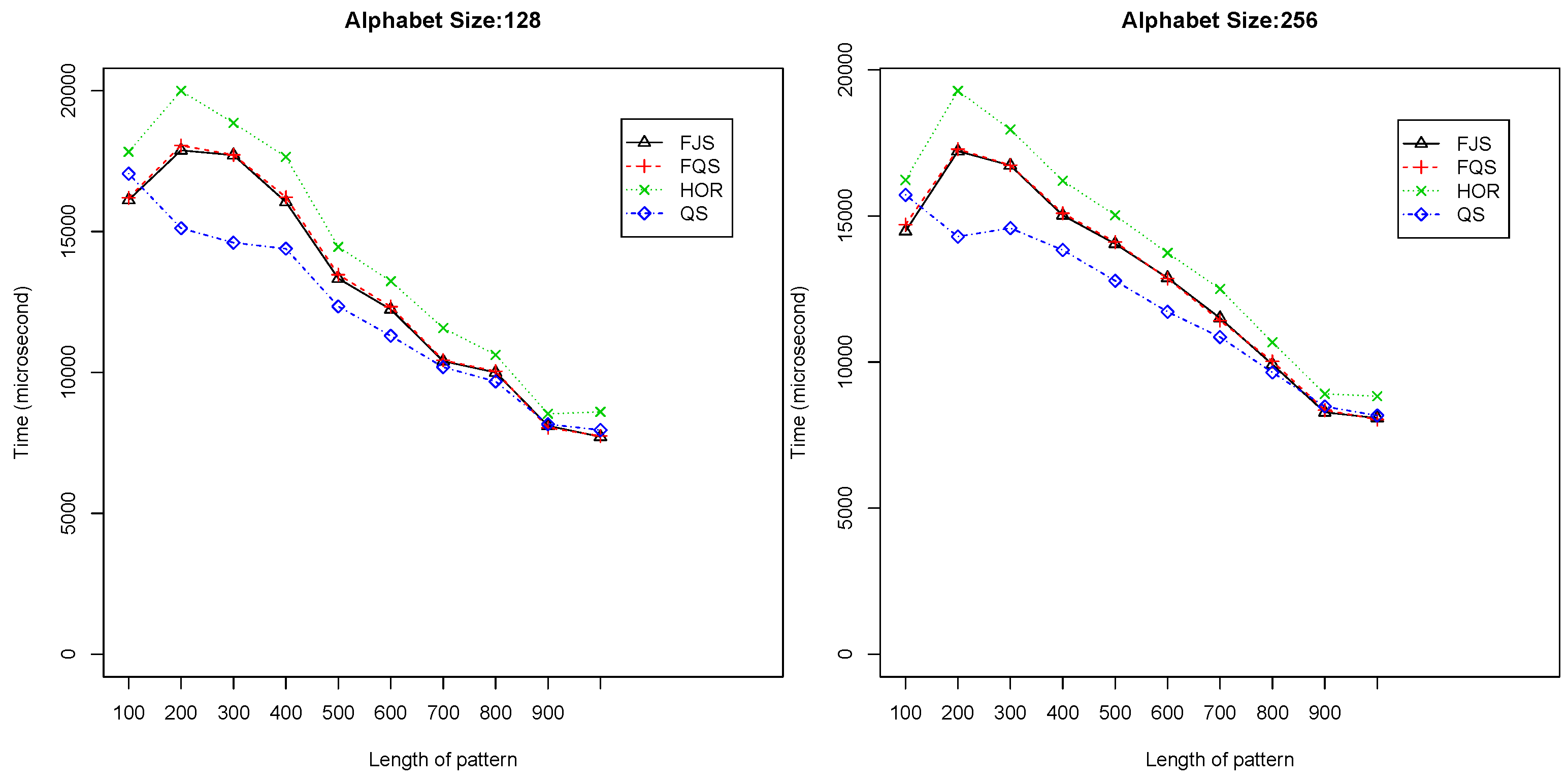
- When and , FQS provides the best results among the four algorithms. Figure 8 shows the comparative results. When the alphabet size is two, four and eight, respectively, QS is the second best. When the alphabet size is 32, and 64, FJS is ranked as the second best, only inferior to FQS;
- When and , QS is the best algorithm; FQS is similar to FJS, ranked as the second. Figure 9 shows the experimental results. When the length of the pattern is longer than 800, QS, FJS and FQS all have a very similar performance.
Figure 6.
Execution time versus pattern length, m (), using randomized text files when .

Figure 7.
Execution time versus pattern length, m (), using randomized text files when . FJS, Franek–Jennings–Smyth; FQS, faster quick search; HOR, Horspool.
Figure 7.
Execution time versus pattern length, m (), using randomized text files when . FJS, Franek–Jennings–Smyth; FQS, faster quick search; HOR, Horspool.

Figure 8.
Execution time versus pattern length, m (), using randomized text files when .
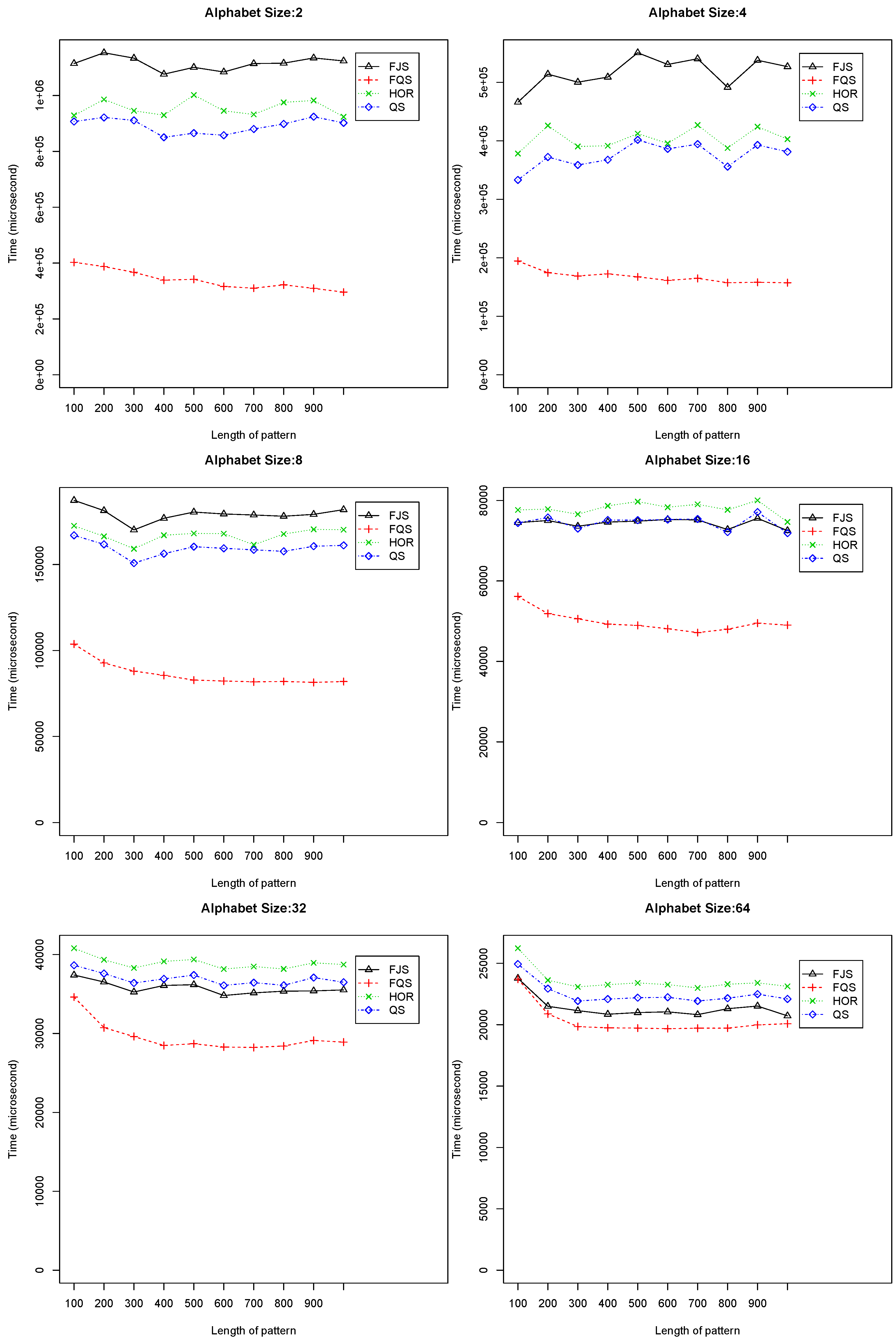
When the alphabet size is small or medium ( = 2, 4, 8, 16, 32 and 64, respectively), the performance of FQS is significantly better than others. When the alphabet size is large ( = 128 or 256), FQS still has a competitive running performance. FQS is suitable to be used with a small or medium alphabet size (not more than 128). The longer the pattern is, the better FQS performs.
Figure 9.
Execution time versus pattern length, m (), using randomized text files when .

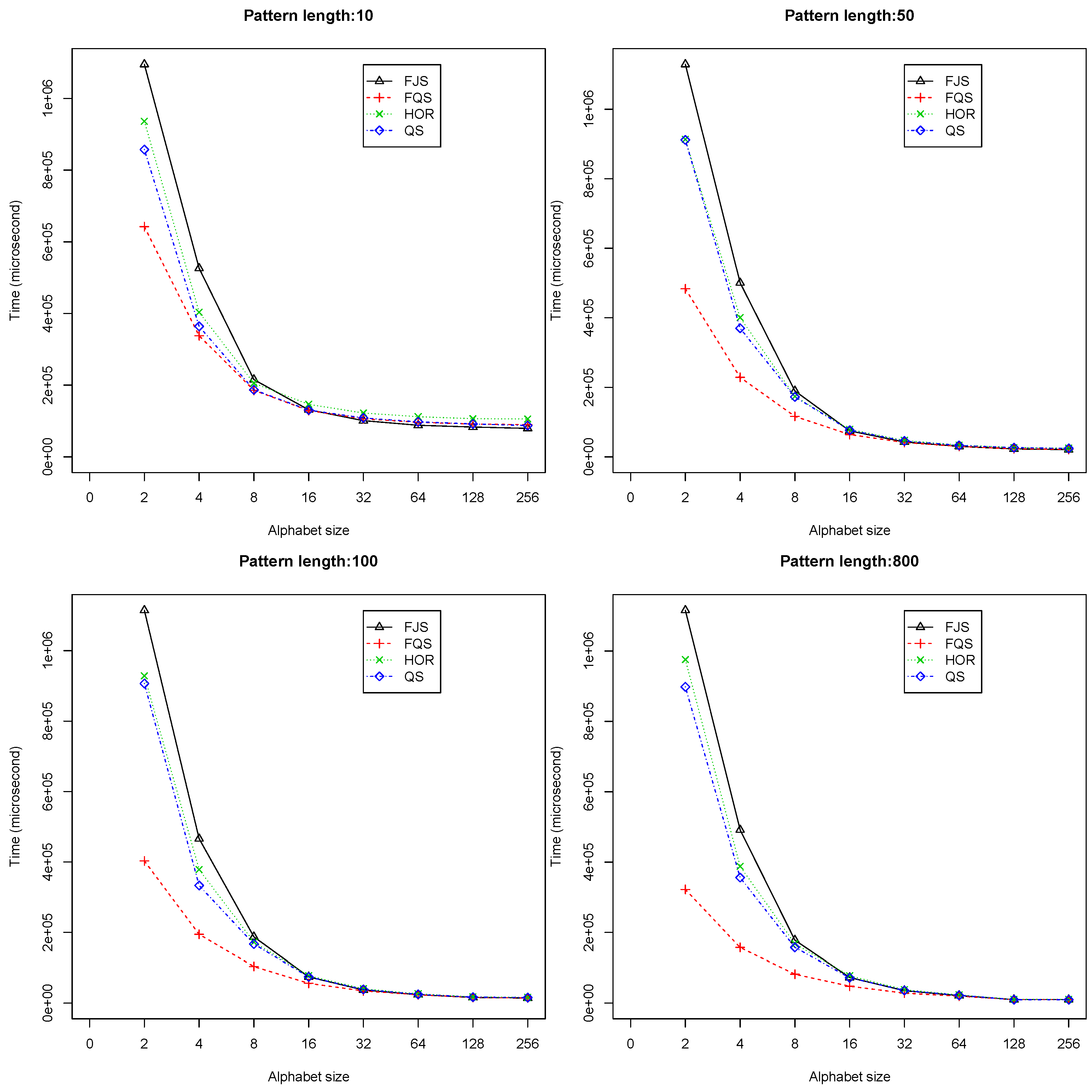
We took a closer look at the impact of alphabet sizes on the performance. Figure 10 shows the average execution time plotted against alphabet size when the pattern length is fixed, for the cases with , , and , respectively.
Figure 10.
The variation of execution time with alphabet size Σ, () using randomized text files, when m = 10, 50, 100 and 800.
Figure 10.
The variation of execution time with alphabet size Σ, () using randomized text files, when m = 10, 50, 100 and 800.

From the figure, we can observe the overall trend for all of the algorithms: with increasing alphabet size , the execution time decreases. FQS has better performance when is small, especially for cases of long patterns (see in Figure 10, for example). This suggests that FQS will have important potential applications in the analysis of a genomic database, since the alphabet size is usually very small, typically four (for DNA or RNA sequences) or 20 (for protein sequences).
We summarize our observations on random texts as follows.
- The longer a pattern is, the faster the FQS algorithm runs;
- When the alphabet size is small or medium ( = 2, 4, 8, 16, 32 and 64), FQS outperforms the other QS variants: Horspool (abbreviated as HOR), FJS and the classic QS;
- When , FQS is competitive with the other QS variants: HOR, FJS and classic QS.
4.2. Practical Text Files
The algorithms were also compared using the following three practical text files downloaded from the Large Canterbury Corpus:
- (1)
- E. coli: the sequence of the Escherichia coli genome consisting of 4,638,690 base pairs with ;
- (2)
- The Bible: The King James version of the Bible consisting of 4,047,392 characters with ;
- (3)
- World192: A CIA World Fact Book consisting of 2,473,400 characters with .
The experiments were carried out the same way as in the case of randomized text files. The same 19 varying pattern lengths are used, namely, m = 10, 20, 30, 40, 50, 60, 70, 80, 90, 100, 200, 300, 400, 500, 600, 700, 800, 900 and 1,000, respectively. For a given pattern length, 50 different patterns are randomly chosen to search in each text file, and the average running time is recorded.
Figure 11 shows the execution time versus pattern length from 10 to 100 in the three practical text files. Figure 12 shows the results for pattern length from 100 to 1,000. In all of these cases, FQS outperforms the others.
Figure 11.
Execution time versus pattern length, m, for short to medium patterns () using practical text files.
Figure 11.
Execution time versus pattern length, m, for short to medium patterns () using practical text files.
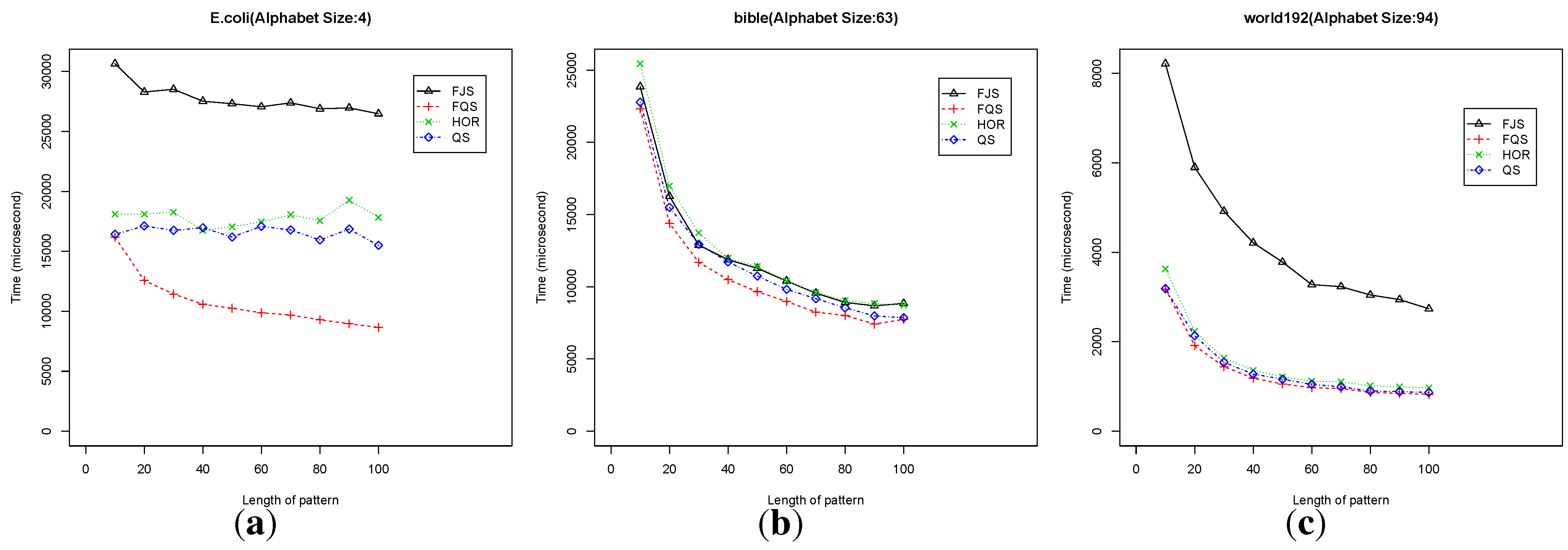
Figure 12.
Execution time versus pattern length, m, for large patterns () using practical text files.
Figure 12.
Execution time versus pattern length, m, for large patterns () using practical text files.

For E. coli, FQS is much better than the other algorithms. The QS and HOR are in the second group rank (Figure 11a and Figure 12a). For the Bible, the four algorithms have a similar performance. FQS is slightly better than the others (Figure 11b and Figure 12b). For World192, QS, FQS and HOR have a similar performance, with FQS showing a slightly better performance (Figure 11c and Figure 12c).
For these practical files, FQS is the overall best algorithm among the four. Each of the three practical files has a symbol alphabet with size . This suggests that FQS might be the algorithm of choice for practical use, especially for searching genomic databases with typically smaller alphabets.
4.3. Number of Symbol Comparisons
To put the practical running times presented above in context, we also investigated the number of comparisons required by the algorithms and the number of pattern shifts performed during the match. These two parameters are the basic determinants of the running time of the algorithms. Below, we report on the performance of the two best algorithms, QS and FQS.
Table 2 shows the number of comparisons, their corresponding standard deviation (STD) and statistical significance (p-value) from algorithms QS and FQS, for pattern lengths m = 10, 100, 500 and 1,000, respectively. From the table, we can observe that, in all cases, the number of comparisons used by FQS is less than that of QS. The Student’s t-test compares whether there is a statistical difference between these two algorithms by using p-value = 0.05 as the threshold. The p-value is shown in bold where there is a significant difference. For Bible and E. coli, there are significant differences in all cases. For World192, there is a statistically significant difference when pattern length m = 1,000; the other three cases (m = 10, 100, 500) do not show any statistically significant difference. Table 3 shows the corresponding results for the number of pattern shifts, the corresponding standard deviation (STD) and statistical difference (p-value) from algorithm QS and FQS, for the pattern lengths m = 10, 100, 500, 1,000. Again, the results show that in all cases, the number of pattern shifts performed by FQS is less than the number for QS. From a statistical point of view, in seven out of 12 cases, there are statistically significant difference in the performance of FQS over QS. Taken together, these two tables provide an explanation for the superior performance of FQS on the practical files when compared with the other QS variants. More importantly, the results show the effectiveness of the innovative use of an intelligent pre-testing stage before embarking on the more time-consuming pattern matching. In our FQS algorithm, this pre-testing is performed using , the location with the maximal expected shift in our FQS algorithm.
| Dataset | m | QS | FQS | p_value | |||
|---|---|---|---|---|---|---|---|
| Mean | STD | Mean | STD | ||||
| Bible | 10 | 2,509,581 | 349,838 | 2,233,411 | 124,671 | 0.0029 | |
| Bible | 100 | 762,316 | 75,952 | 646,298 | 54,656 | <0.01 | |
| Bible | 500 | 436,243 | 69,142 | 366,246 | 52,643 | 0.0010 | |
| Bible | 1,000 | 371,849 | 47,702 | 311,520 | 45,886 | 0.0002 | |
| E. coli | 10 | 1,595,760 | 345,988 | 1,197,866 | 265,086 | 0.0002 | |
| E. coli | 100 | 1,634,972 | 548,912 | 657,987 | 128,279 | <0.01 | |
| E. coli | 500 | 1,563,532 | 435,567 | 541,158 | 75,234 | <0.01 | |
| E. coli | 1,000 | 1,777,232 | 505,260 | 538,972 | 87,332 | <0.01 | |
| World192 | 10 | 314,182 | 44,298 | 307,453 | 30,050 | 0.5777 | |
| World192 | 100 | 75,189 | 11,321 | 70,636 | 11,953 | 0.2238 | |
| World192 | 500 | 33,607 | 6,834 | 30,483 | 6,272 | 0.1403 | |
| World192 | 1,000 | 26,898 | 4,649 | 23,800 | 3,675 | 0.0250 | |
| Dataset | m | QS | FQS | p_value | |||
|---|---|---|---|---|---|---|---|
| Mean | STD | Mean | STD | ||||
| Bible | 10 | 2,091,864 | 88,154 | 1,981,448 | 170,460 | 0.0156 | |
| Bible | 100 | 668,353 | 53,648 | 638,690 | 54,324 | 0.0904 | |
| Bible | 500 | 395,943 | 45,934 | 361,286 | 52,932 | 0.0332 | |
| Bible | 1,000 | 336,126 | 48,988 | 304,023 | 46,194 | 0.0395 | |
| E. coli | 10 | 1,173,807 | 274,324 | 1,060,892 | 235,219 | 0.1706 | |
| E. coli | 100 | 1,220,728 | 410,989 | 603,276 | 119,927 | <0.01 | |
| E. coli | 500 | 1,167,201 | 326,151 | 497,990 | 69,480 | <0.01 | |
| E. coli | 1,000 | 1,326,734 | 378,141 | 495,055 | 79,672 | <0.01 | |
| World192 | 10 | 285,185 | 29,089 | 265,368 | 29,591 | 0.0392 | |
| World192 | 100 | 71,759 | 11,011 | 70,235 | 12,103 | 0.6794 | |
| World192 | 500 | 31,265 | 6,038 | 29,869 | 6,252 | 0.4768 | |
| World192 | 1,000 | 24,299 | 4,146 | 22,650 | 3,672 | 0.1910 | |
4.4. Statistical Analysis
We applied the Student’s t-test to compare FQS vs. FJS, FQS vs. HOR and FQS vs. QS in 19 varied pattern lengths using randomized files and three practical files. The testing results are shown in Figure 13. The x-axis represents the 19 varied pattern lengths (m); the y-axis is arranged accordingly with the alphabet size (11 total cases). From the figure, we can find that the statistical testing results match with the previous performances well. In most cases, FQS performed better than FJS, HOR and QS.
Figure 13.
The Student t-test for: (a) FQS vs. FJS (b) FQS vs. HOR and (c) FQS vs. QS in the condition of execution time versus pattern length, m. “B” denotes cases when FQS has a statistically significant better performance over the comparison algorithm; “S” denotes cases where FQS and the comparison algorithm have statistically the same performance; “W” denotes cases where FQS has a statistically significant worse performance than the comparison algorithm.
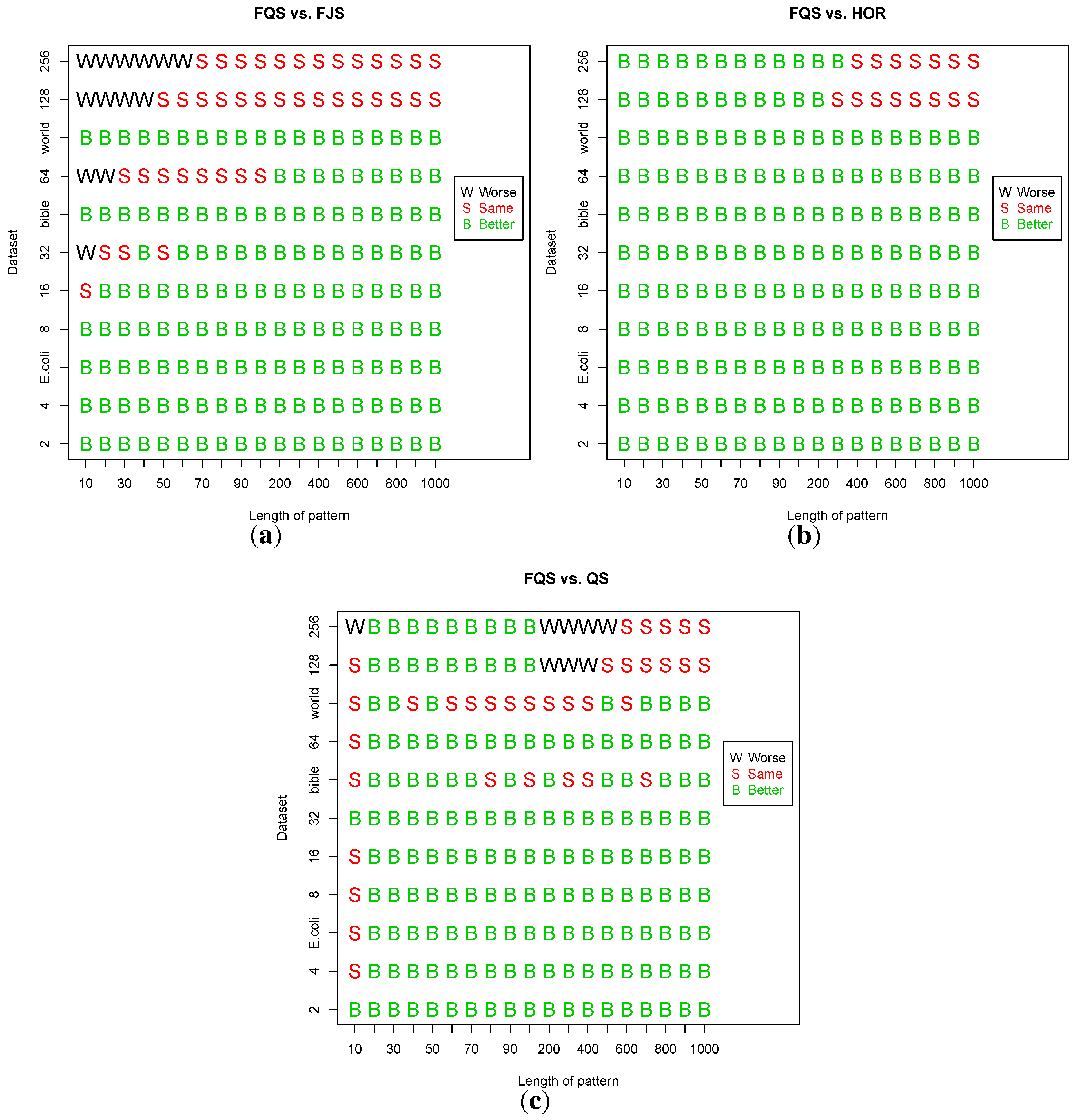
Let us examine Figure 13a in the figure. There are 209 (19 × 11) total comparison cases: FQS performed better than FJS in 156 cases with statistically significant differences; they had the same performance in 40 cases; FJS had better performance in 13 cases. FJS performed better in cases when : (1) and ; (2) and ; (3) and ; (4) and ;
When comparing FQS vs. HOR (Figure 13b), in a total of 209 cases, both had statically the same performance in 15 cases, and FQS outperformed HOR in the other 194 cases. Comparing FQS vs. QS (Figure 13c), FQS was statistically worse than QS in eight cases; both had similar performance in 34 cases, and FQS showed a statistically better performance in the remaining 167 cases.
5. Conclusions
The FQS algorithm improves on the quick search (QS) algorithm, by applying the bad character rule, aided with a statistically maximal expected shift value introduced in this work and a pre-testing stage before full pattern matching. Unlike previous approaches that blindly tested the first and last symbols in the pattern [20,21], our pre-testing stage is performed by computing the statistical maximal expected shift position. We have compared FQS against three other competitive QS variants: the QS itself, FJS and the Horspool algorithm. A range of text files were searched, including randomly generated text files with different alphabet sizes (), and practical benchmark text files, namely E. coli, Bible and World192, from the Canterbury Corpus. The pattern lengths were varied from 10 to 1,000 with 19 varieties. We find that, statistically, FQS has the overall best performance (practical running time, number of symbol comparisons and number of pattern shifts) over all of the other three algorithms, mostly especially for text files with alphabet sizes less than 128. The results suggest that FQS could have important applications in practice, especially for genomic data sets, such as DNA or RNA sequences with four symbols or protein sequences with 20 symbols.
Acknowledgments
This work was supported in part by a grant from the U.S. National Science Foundation: IIS-1236983.
Author Contributions
JL conceived of and implemented the algorithm. DA and YJ helped to draft the manuscript. All authors read and approved the final manuscript.
Conflicts of Interest
The authors declare no conflict of interest.
References
- Charras, C.; Lecroq, T. Handbook of Exact String Matching Algorithms; College Publications: London, UK, 2004. [Google Scholar]
- Smyth, W. Computing Patterns in Strings; Addison-Wesley: Boston, MA, USA, 2003. [Google Scholar]
- Knuth, D.; Morris, J.; Pratt, V. Fast pattern matching in strings. SIAM J. Comput. 1977, 6, 323–350. [Google Scholar] [CrossRef]
- Karp, R.M.; Rabin, M.O. Efficient Randomized Pattern-matching Algorithms. IBM J. Res. Dev. 1987, 31, 249–260. [Google Scholar] [CrossRef]
- Boyer, R.; Moore, J. A fast string searching algorithm. Commun. ACM 1977, 20, 62–72. [Google Scholar] [CrossRef]
- Baeza-Yates, R.; Gonnet, G. A new approach to text searching. Commun. ACM 1992, 35, 74–82. [Google Scholar] [CrossRef]
- Fredriksson, K.; Grabowski, S. Average-optimal string matching. J. Discret. Algorithms 2009, 7, 579–594. [Google Scholar] [CrossRef]
- Kuei-Hao Chen, G.S.H.; Lee, R.C.T. Bit-Parallel Algorithms for Exact Circular String Matching. Comput. J. 2014, 57, 731–743. [Google Scholar] [CrossRef]
- Faro, S.; Lecroq, T. The Exact Online String Matching Problem: A Review of the Most Recent Results. ACM Comput. Surv. 2013, 45, 13:1–13:42. [Google Scholar] [CrossRef]
- Sunday, D. A Very Fast Substring Search Algorithm. Commun. ACM 1990, 33, 132–142. [Google Scholar] [CrossRef]
- Apostolico, A.; Crochemore, M. Optimal Canonization of All Substrings of a String. Inf. Comput. 1991, 95, 76–95. [Google Scholar] [CrossRef]
- Crochemore, M.; Rytter, W. Text Algorithms; Oxford University Press: Oxford, UK, 1994. [Google Scholar]
- Franek, F.; Jennings, C.G.; Smyth, W.F. A simple fast hybrid pattern-matching algorithm. J. Discret. Algorithms 2007, 5, 682–695. [Google Scholar] [CrossRef]
- Horspool, R.N. Practical fast searching in strings. Softw. Pract. Exp. 1980, 10, 501–506. [Google Scholar] [CrossRef]
- Gusfield, D. Algorithms on Strings, Trees and Sequences: Computer Science and Computational Biology; Cambridge University Press: Cambridge, UK, 1997. [Google Scholar]
- Adjeroh, D.; Bell, T.; Mukherjee, A. The Burrows-Wheeler Transform: Data Compression, Suffix Arrays and Pattern Matching; Springer: Berlin, Germany, 2008. [Google Scholar]
- Adjeroh, D.A.; Bell, T.; Mukherjee, A. Pattern Matching in Compressed Texts and Images. Found. Trends Signal Process. 2013, 6, 97–241. [Google Scholar] [CrossRef]
- Galil, Z. On improving the worst case running time of the Boyer-Moore string matching algorithm. In Commun. ACM 1979, 22, 505–508. [Google Scholar] [CrossRef]
- Apostolico, A.; Giancarlo, R. The Boyer Moore Galil string searching strategies revisited. SIAM J. Comput. 1986, 15, 98–105. [Google Scholar] [CrossRef]
- Sheik, S.; Aggarwal, S.; Poddar, A.; Balakrishnan, N.; Sekar, K. A fast pattern matching algorithm. J. Chem. Inf. Comput. 2004, 44, 1251–1256. [Google Scholar] [CrossRef] [PubMed]
- Thathoo, R.; Virmani, A.; Lakshmi, S.S.; Balakrishnan, N.; Sekar, K. TVSBS: A fast exact pattern matching algorithm for biological sequences. Curr. Sci. 2006, 91, 47–53. [Google Scholar]
- Raita, T. Tuning the Boyer-Moore-Horspool String Searching Algorithm. Softw. Pract. Exp. 1992, 22, 879–884. [Google Scholar] [CrossRef]
© 2014 by the authors. Licensee MDPI, Basel, Switzerland. This article is an open access article distributed under the terms and conditions of the Creative Commons Attribution license ( http://creativecommons.org/licenses/by/3.0/).
Share and Cite
MDPI and ACS Style
Lin, J.; Adjeroh, D.; Jiang, Y. A Faster Quick Search Algorithm. Algorithms 2014, 7, 253-275. https://doi.org/10.3390/a7020253
AMA Style
Lin J, Adjeroh D, Jiang Y. A Faster Quick Search Algorithm. Algorithms. 2014; 7(2):253-275. https://doi.org/10.3390/a7020253
Chicago/Turabian StyleLin, Jie, Donald Adjeroh, and Yue Jiang. 2014. "A Faster Quick Search Algorithm" Algorithms 7, no. 2: 253-275. https://doi.org/10.3390/a7020253