Pressure Model of Control Valve Based on LS-SVM with the Fruit Fly Algorithm

Abstract

Control valve is a kind of essential terminal control component which is hard to model by traditional methodologies because of its complexity and nonlinearity. This paper proposes a new modeling method for the upstream pressure of control valve using the least squares support vector machine (LS-SVM), which has been successfully used to identify nonlinear system. In order to improve the modeling performance, the fruit fly optimization algorithm (FOA) is used to optimize two critical parameters of LS-SVM. As an example, a set of actual production data from a controlling system of chlorine in a salt chemistry industry is applied. The validity of LS-SVM modeling method using FOA is verified by comparing the predicted results with the actual data with a value of MSE 2.474 × 10⁻³. Moreover, it is demonstrated that the initial position of FOA does not affect its optimal ability. By comparison, simulation experiments based on PSO algorithm and the grid search method are also carried out. The results show that LS-SVM based on FOA has equal performance in prediction accuracy. However, from the respect of calculation time, FOA has a significant advantage and is more suitable for the online prediction.

1. Introduction

The control valve is a common element in modem process control, which is used to control the flow of a fluid. Its mathematical model is usually necessary in designing the automatic control or fault diagnosis systems. Song K. et al. [1,2] described the system of control valve based on fluid mechanics. However, there are a lot of limitations for the theory analysis method because of the complexity of the structure, nonlinearity and time-lag of the control valve. This makes it is quite difficult to accurately forecast the physical variable of control valve. To overcome this problem, some simulation calculation methods are used, such as bondgraph approach [3] and system identification. Especially the latter is wildly used. J.W. Ma [4] predicted the characteristics of hydraulic valve using support vector machine. A. Helling [5] deduced the dynamic mathematic model of the control valve using neural network.

The least squares support vector machine (LS-SVM) is a reformulation of the support vector machine (SVM) which solves linear programming problem rather than quadratic programming problem [6,7]. LS-SVM can approach the nonlinear system with high precision, making it an excellent method for modeling nonlinear systems [8,9]. The LS-SVM model has been successfully used to solve forecasting problems in many fields, such as CO concentration [10], gas [11,12], short term electric load [13,14,15], revenue [16], precipitation [17], wind speed [18], hydropower consumption forecasting [19], and so on. However, we regret that few literatures study the modeling of control valve using LS-SVM. This paper explores the feasibility of using the LS-SVM model to forecast the upstream pressure of control valve. The forecasting performance of the LS-SVM model largely depends on the values of its two parameters. Currently, several meta-heuristic algorithms have been used to determine the optimal values of these two parameters, including particle swarm optimization [11], genetic algorithm [12], chaotic differential evolution approach [20], artificial bee colony algorithm [21], and simulated annealing algorithm [22]. However, these algorithms have some drawbacks such as being hard to understand and reaching the global optimal solution slowly.

The fruit fly optimization algorithm (FOA) is a novel evolutionary optimization technique, which was proposed by Pan in 2011 [23]. This new optimization algorithm has the advantages of being easy to understand and of reaching the global optimal solution fast. Recently, the FOA has been applied for different problems, for example PID controller tuning [24], power load forecasting [25,26], web auction logistics service [27] and financial distress [23]. Therefore, this paper attempts to use the FOA to optimize the two necessary parameters in order to improve the performance of the LSSVM model in upstream pressure forecasting of the control valve.

The outline of the paper is as follows. Section 2 introduces the physical model and LS-SVM model of upstream pressure. Section 3 studies the influence of the LS-SVM parameters on identification performance. Then, in Section 4, the process of optimizing the parameters of LS-SVM based on FOA is introduced in detail. Section 5 introduces the method of sampling the test data, the predicting results and comparison between FOA, the particle swarm optimization (PSO) and the grid search method. Finally, the proposed modeling method is concluded in Section 6.

2. LS-SVM Upstream Pressure Model of Control Valve

2.1. Physical Model of the Upstream Pressure of Control Valve

The upstream pressure adjusting equation of the control valve can be deduced from the physical properties of the fluid and the restriction characteristics [28], that is:

(1)

where p₁ is the upstream pressure, p₂ is the downstream pressure, q is the flow rate, ρ is the mean density of fluid, β is ratio of contractive section diameter to the pipe diameter, ε is the expansion factor which is influenced by the temperature T, A_r is the area of contractive section which is the function of the opening of the control valve (%) and E is velocity coefficient.

From Equation (1), the upstream pressure can be written as a function f of the physical properties of the fluid and control valve in Equation (2):

p₁ = f(p₂,q,T,%)

(2)

Now, if the non-linear relation in Equation (2) is known, the upstream pressure of control valve can be obtained by simply measuring the downstream pressure, the flow rate, temperature and the percentage of opening of the control valve. However, the computational calculations of the upstream pressure from Equation (2) may not be practical for the real-time control of the upstream-pressure-control valve due to the strong non-linearity and complexity. To overcome this problem, the LS-SVM is used to capture the relationship between the upstream pressure and the properties of the fluid and the control valve.

2.2. Introduction to LS-SVM

LS-SVM is a kind of learning machine which can estimate the relationships between input and output of a system. The algorithm is as follows:

Given a training sample set (x_i, y_i), i = 1, 2,···, l, where x_i ∈ Rⁿ is the input values, y_i ∈ R is the output values and l is the number of the samples. First, the sample set is mapped to a high-dimensional feature space R^nh from the original space Rⁿ through a nonlinear mapping. Then, an optimal linear regression function f(x) = ωφ(x) + b is constructed in the high-dimensional space. According to structure risk minimization, ω and b can be obtained from minimizing J = ||ω||² + CE. Where φ(x) is the feature map mentioned above, J is the regularized cost function, ω is the weight vector of the high dimensional feature space, ||ω||² = ω^Tω is the complexity of algorithm model, b is the deviation, C is the regularization constant and E is the loss function using the quadratic term of the slack variable ξ. The regression problem of function can be represented as the optimization problem of the regularized cost function J:

(3)

To solve the optimization problem of Equation (3), a Lagrange function is constructed:

(4)

where α_i are Lagrange multipliers. The conditions for optimality are:

(5)

Equation (5) can be rewritten as:

(6)

After contracting ω and ξ_i, we get:

(7)

According to the Mercer’s condition, there is the kernel function as:

K(x,x_i) = ϕ(x)ϕ(x_i)

(8)

Then we can obtain the estimate LS-SVM function of the upstream pressure in Equation (2) as:

(9)

where x ∈ R⁴ is the input variables including p₂, q, T, %. Lagrange multipliers α_i and the deviation b are obtained from the set of linear Equation (7). The kernel function can be any symmetric function satisfying the mercer condition. Typical examples are linear kernel, polynomial kernel and radical basis function (RBF). In this study, the RBF kernel function K(x,x_i) = exp[−||x − x_i||²/(2σ²)] is used. Consequently, there are two sensitive parameters in the estimation of LS-SVM including the regularization constant C and kernel bandwidth σ.

3. Influence of the LS-SVM Parameters on Identification Performance

The performance of LS-SVM with RBF kernel function is influenced by the regularization constant C and kernel bandwidth σ. C is introduced to measure the trade-off between complexity and losses. It adjusts empirical risk and confidence interval to lead to a good generalization performance. If the value is too small, the punishment of error is small, which makes big training error and poor generalization ability. If the value is too big, then only the risk of experience is minimized but the complexity of the model is not considered, which will also bring poor generalization ability. Smaller σ might yield the SVM over trained and make the kernel matrix trend toward unit matrix. On the contrary, bigger σ will make the kernel function tend to be constant.

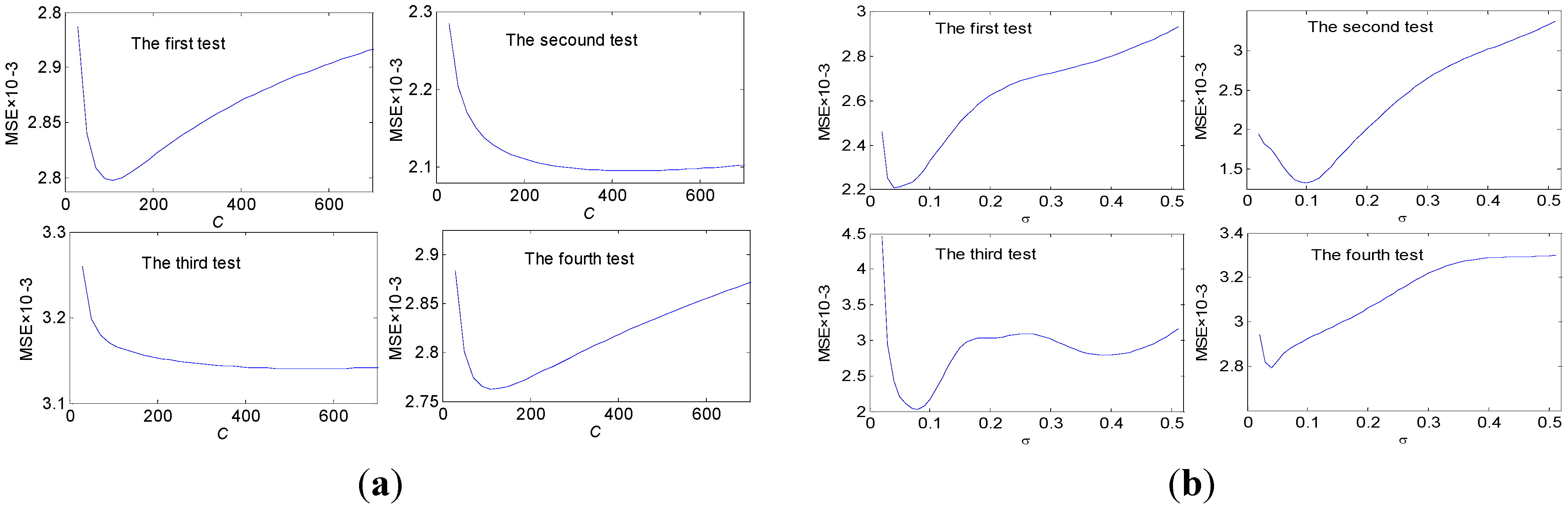
In order to contrast the influences of different C and σ, simulated tests are carried out four times respectively. The sampling set is from an actual pressure control system of chlorine in a salt industry plant which will be introduced in Section 5. Six hundred sample data are randomly divided into five groups. Among them, four groups are the training data and the other group is the test data. The mean squared error (MSE) is used to estimate the forecast accuracy.

In the first set of experiments σ is fixed at 0.04 while the value of C is varied. Then in the second set of experiments C is set to 200 while the different σ values are tested. The relationships of MSE versus C and σ are displayed in Figure 1a,b respectively. The values of C and σ that minimize MSE are listed in Table 1. It can be observed from Figure 1 and Table 1: Firstly, for the fixed sampling data set, different parameter values (e.g., C of the first test in Figure 1a) make the performance of LS-SVM different. There is an optimal parameter value minimizing the MSE. Secondly, the test data is different among the four times experiments because of they are fetched randomly from the sample set. Moreover, the optimal parameter values of four times are also different. Thereby, we can draw the conclusion that the optimal parameter value varies with the sample data, even for the same predicting object. In brief, to get the best modeling performance, it is necessary to optimize the parameters C and σ before every regression for any data set.

Figure 1. Prediction accuracy versus parameters. (a) versus C (σ = 0.04); (b) versus σ (C = 200).

Figure 1. Prediction accuracy versus parameters. (a) versus C (σ = 0.04); (b) versus σ (C = 200).

Table 1. The optimal parameters for different training and test sampling.

Test Number	1	2	3	4
Optimal C (σ = 0.04)	110	430	550	110
Optimal σ (C = 200)	0.04	0.10	0.8	0.04

Table 1. The optimal parameters for different training and test sampling.

Test Number	1	2	3	4
Optimal C (σ = 0.04)	110	430	550	110
Optimal σ (C = 200)	0.04	0.10	0.8	0.04

4. Optimize Parameters of LS-SVM Employing Fruit Fly Optimization Algorithm

Fruit Fly Optimization Algorithm (FOA) is a new approach for finding global optimization based on the food finding behavior of the fruit fly [23].

The process of optimizing the parameters C and σ using FOA is divided as follows and the flow diagram is illustrated in Figure 2 [25,29,30].

Figure 2. The flow diagram of fruit fly optimization algorithm (FOA).

Figure 2. The flow diagram of fruit fly optimization algorithm (FOA).

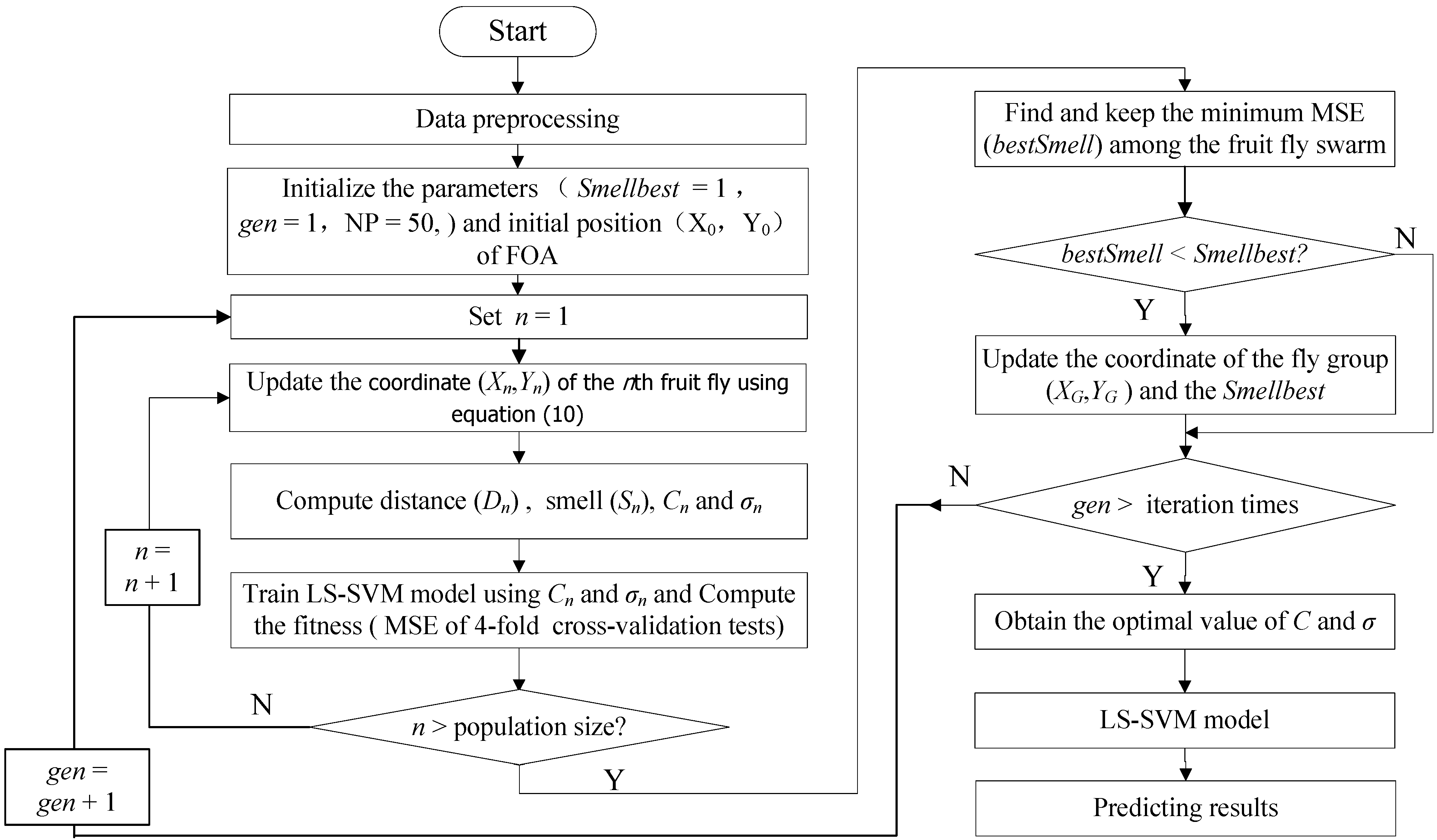
Step 1. Data preprocessing, mainly including normalization processing and dividing the sample data into training data and test data.

Step 2. Initialize the parameters and the initial position of FOA: first, set the maximum number of generations (gen), the initial value of Smellbest (bigger enough than the actual max MSE) and population size (NP); and second, randomly initial fruit fly group location (X_G, Y_G) = (X₀, Y₀).

Step 3. Give the random direction η and swarm radius R. The coordinates of the nth fruit fly (X_n,Y_n ) is:

X_n = X_G + R(η − 0.5)    Y_n = Y_G + R(η − 0.5)

(10)

where n = 1, 2, …, NP and η ∈ [0,1] is a random number.

Step 4. Because the food location cannot be known, the distance to the origin is estimated first (D_n), then the smell concentration judgment value (S) is calculated whose value is the reciprocal of distance and C_n, σ_n can be calculated.

(11)

Step 5. Train LS-SVM model using σ_n, C_n and then conduct the 4-fold cross-validation tests. The smell concentration judgment function (or called fitness function) is defined as:

(12)

where m is the number of the data in every sample subset, ŷ_ij is the predicted value and y_ij is the actual value.

Step 6. Find out the fruit fly with the minimum Smell value in the whole fly swarm and its index among the fruit fly swarm.

[bestSmell  bestIndex] = min(Smell)

(13)

Step 7. Judge if the bestSmell is superior to the previous Smellbest, if so, the fruit fly swarm will use vision to fly towards that location. The Smellbest and the coordinate of the fly group (X_G, Y_G) are updated:

Smellbest = bestSmell, X_G = X(bestIndex), Y_G = Y(bestIndex)

(14)

Otherwise, go to step 8.

Step 8. Judge if the iteration is end, if not, go to step 3 and continue to cycle. Otherwise, obtain the optimal values of C and σ, and begin to predict using LS-SVM.

According to the iteration steps above, there are only three parameters to be set including the population size, the initial position of population and the maximum iteration times.

5. Modeling Design of LS-SVM Based on FOA and Simulation Test

5.1. Sampling Data

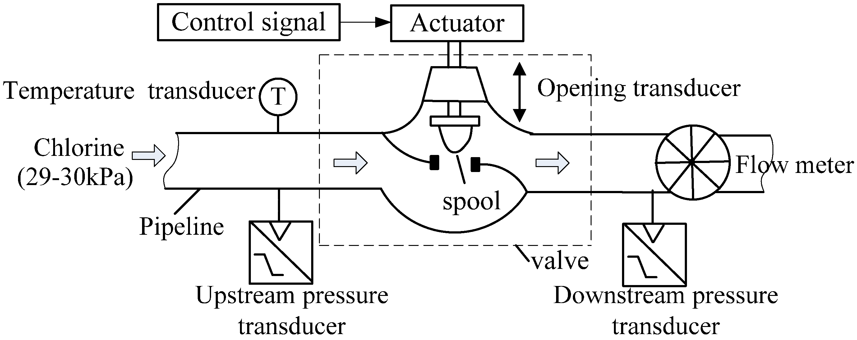
As an example, a sample set from an actual pressure control system of chlorine in a salt industry plant (shown in Figure 3) is used to model the upstream pressure of the control valve. In order to maintain a normal production, the pressure of the chlorine pipeline should be maintained between 29–30 KPa. This is accomplished by a control valve. Its opening is adjusted according to the actual production situation to guarantee the needed upstream pressure. In the process of production, the temperature of chlorine changes little and the downstream pressure is influenced by the upstream pressure, opening and the flow rate. Consequently, in order to improve the computing speed, the simulation test uses the opening and the flow rate as the input data to predict the upstream pressure. The test results shown in Section 5.2 indicate that using the two independent variables can reach a satisfactory accuracy.

A set of 600 data is sampled in the process of commissioning by the DCS every 20 s. Table 2 shows the descriptive statistical values of the indexes. The data set is divided averagely into five groups. Among them, four groups are used as training data and the other group is used to test the model.

Figure 3. Diagram of chlorine pressure control system.

Figure 3. Diagram of chlorine pressure control system.

Table 2. The descriptive statistical values of the test data.

Factor	Max	Min	Avg	Std
flow rate (Nm3/h)	3666.3	1068.9	2256.3	920.6342
Opening (%)	61.9	36.2	48.2	8.6493
upstream pressure(kPa)	22.81	16.64	19.75	1.9464

Table 2. The descriptive statistical values of the test data.

Factor	Max	Min	Avg	Std
flow rate (Nm3/h)	3666.3	1068.9	2256.3	920.6342
Opening (%)	61.9	36.2	48.2	8.6493
upstream pressure(kPa)	22.81	16.64	19.75	1.9464

5.2. Simulation Result and Analysis

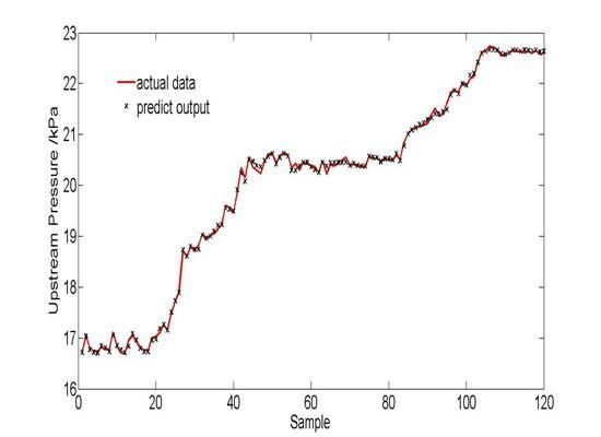
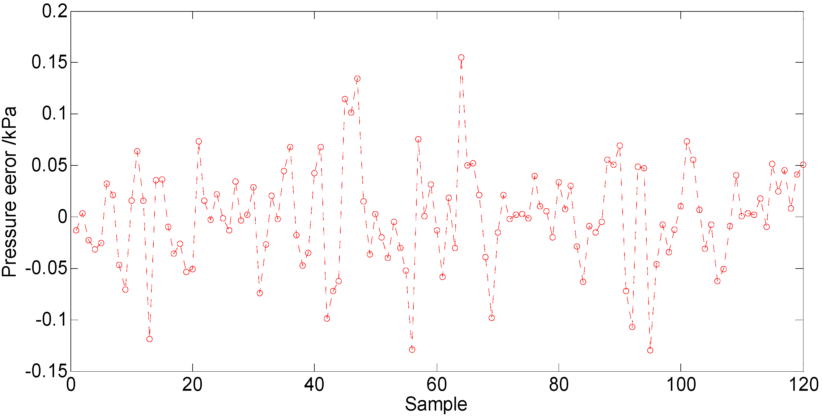
The upstream pressure of control valve shown in Figure 3 is modeled using LS-SVM. The parameters σ and C are optimized using the proposed FOA. The population size is 10 and the iteration number is 50. The mean square error (MSE) is calculated as the smell concentration judgment function (or called fitness function). The optimal values of parameters are: σ = 102.6146, C = 0.0410. The simulation results are shown in Figure 4 and Figure 5. Figure 4 is comparison of the predicted value and the actual output and Figure 5 is the estimated errors curve. The MSE value is 2.474 × 10⁻³ and the mean absolute error (MAE) is 0.808 × 10⁻³ kPa. These indicate that the presented approach shows a quite satisfactory accuracy.

Figure 4. Comparison between the actual values and predict output.

Figure 4. Comparison between the actual values and predict output.

Figure 5. Output errors of upstream pressure.

Figure 5. Output errors of upstream pressure.

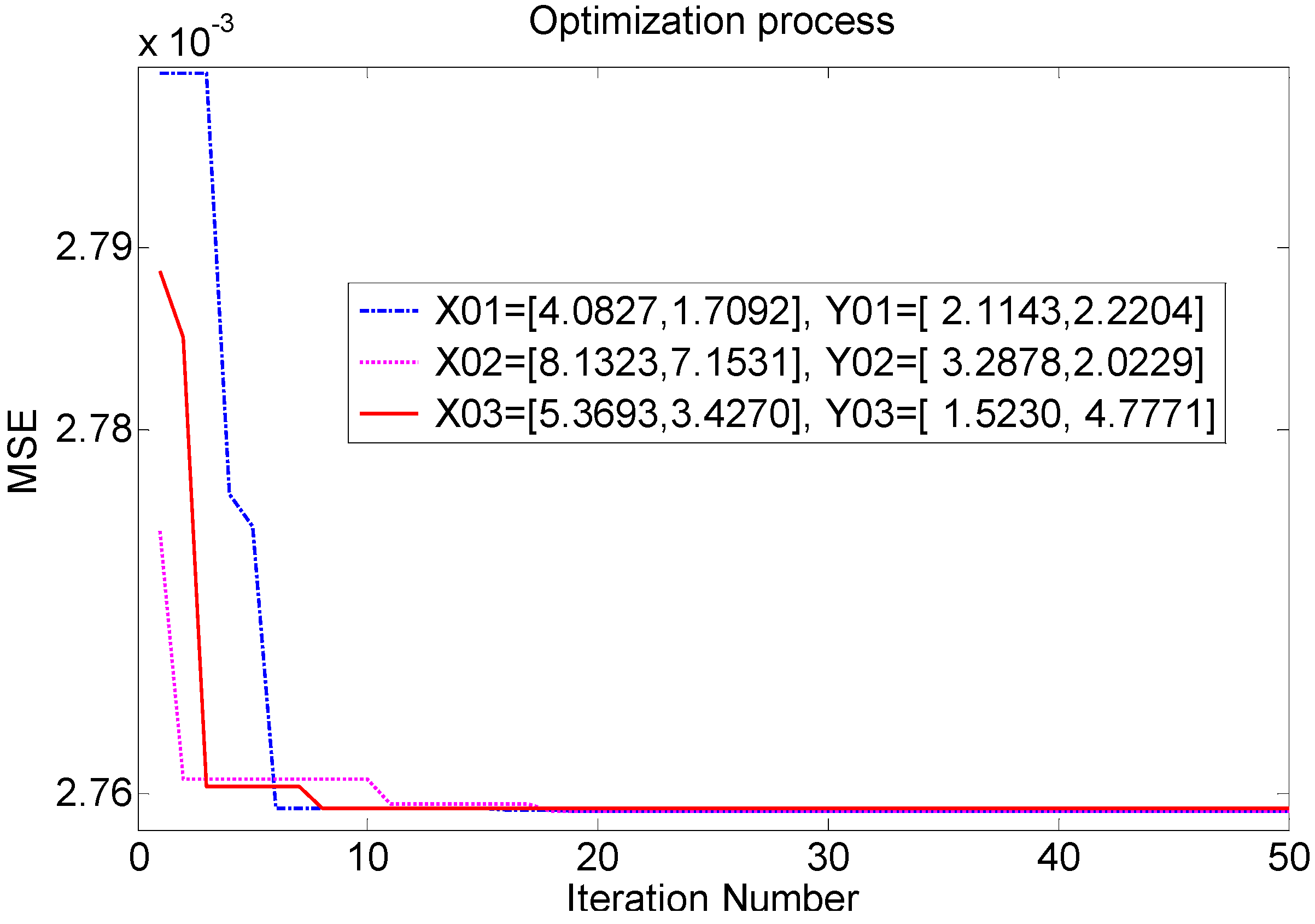
The convergence histories of three different fruit fly swarm initial positions (X₀ and Y₀ which are obtained randomly in the interval [0, 10]) are compared in Figure 6. Table 3 gives their corresponding optimal performances. In Figure 6, the three smell concentrations (minimum mean square error, MSE) of the first iteration are different because of their various initial positions. Nevertheless, all the three lines decline sharply at the early stage of iterations and eventually converged to a steady. In Table 3, it can be found that three optimal results (values of C and σ) and computing time are almost the same, and the three MSE values of predicting the upstream pressure using the optimal C and σ are basically the same too. This indicates that the initial position of the fruit fly swarm does not affect the optimal speed, the optimal results, the computing time and the accuracy of prediction basically.

Figure 6. Convergence histories of different initial positions.

Figure 6. Convergence histories of different initial positions.

Table 3. Influence of different fruit fly initial position.

No.	X0	Y0	C	σ	t/s	MSE/×10
1	[4.0827,1.7092]	[2.1143,2.2204]	91.6280	0.0367	37.6	2.8696
2	[8.1323,7.1531]	[3.2878,2.0229]	92.0664	0.0368	32.5	2.8696
3	[5.3693,3.4270]	[1.5230,4.7771]	93.1784	0.0373	33.0	2.8697

Table 3. Influence of different fruit fly initial position.

No.	X0	Y0	C	σ	t/s	MSE/×10
1	[4.0827,1.7092]	[2.1143,2.2204]	91.6280	0.0367	37.6	2.8696
2	[8.1323,7.1531]	[3.2878,2.0229]	92.0664	0.0368	32.5	2.8696
3	[5.3693,3.4270]	[1.5230,4.7771]	93.1784	0.0373	33.0	2.8697

At present, in the area of parameter optimization, particle swarm optimization (PSO) algorithm is the most frequently studied and is widely applied, and the grid search method is the simplest algorithm. In this article, parameters of C and σ are also optimized by PSO and the grid search algorithm respectively. The scope of C is [2⁻¹⁰, 2¹⁰] and that of σ is [0, 0.2]. Without loss of generality, the iteration times of the two algorithms are set to be 50 and number of particle is 10, which are the same with FOA. Comparison of the convergence histories is shown in Figure 7 and the predicting performance indicators are listed in Table 4 in which MSE are the mean square error, MAE are the mean absolute error.

Figure 7 shows that FOA has faster convergence speed and equal optimal result compared with the other two algorithms. The test indicators in Table 4 further improve the above conclusion. All the three methods could give good LSSVM parameters with offering small MSE and MAE as shown in Table 4. They are equal in forecasting performance. However, from the time consuming point of view, FOA has a significant advantage. Therefore, FOA is more suitable for the online prediction of the pressure of control valve.

Figure 7. Convergence histories of least squares support vector machine (LS-SVM) parameters using different optimization algorithms.

Figure 7. Convergence histories of least squares support vector machine (LS-SVM) parameters using different optimization algorithms.

Table 4. Prediction performances using FOA, PSO and grid search.

Optimization Method	MSE/×10−3	MAPE/%	MSE/×10−3kPa	Error Range/kPa	t/s
FOA	2.474	0.1896	0.808	[−0.69, 0.77]	27.253
PSO	2.462	0.1888	1.043	[−0.71, 0.76]	43.649
Grid Search	2.497	0.1906	1.024	[−0.71, 0.77]	50.451

Table 4. Prediction performances using FOA, PSO and grid search.

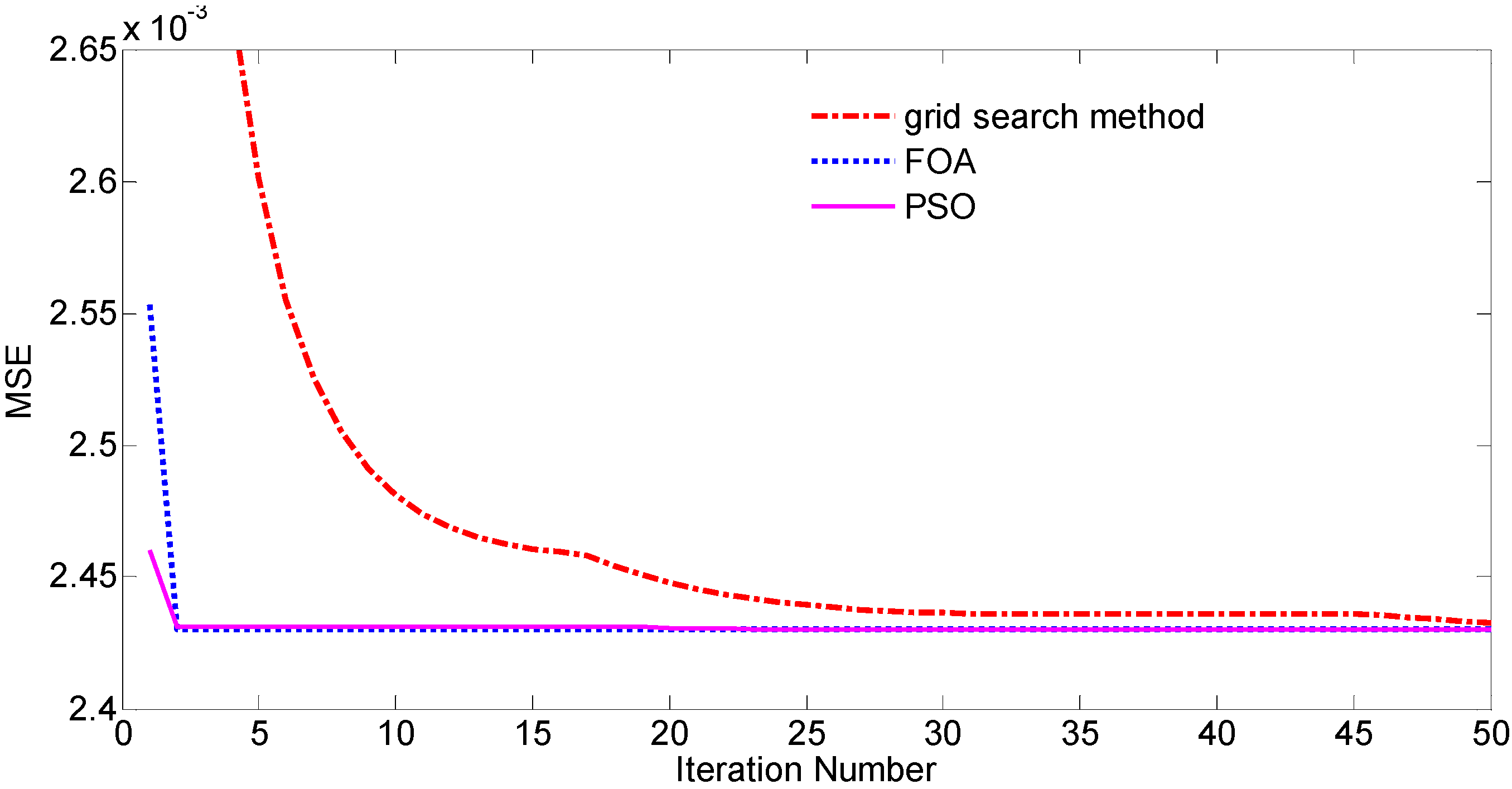
Optimization Method	MSE/×10−3	MAPE/%	MSE/×10−3kPa	Error Range/kPa	t/s
FOA	2.474	0.1896	0.808	[−0.69, 0.77]	27.253
PSO	2.462	0.1888	1.043	[−0.71, 0.76]	43.649
Grid Search	2.497	0.1906	1.024	[−0.71, 0.77]	50.451

6. Conclusions

A new modeling method of control valve based on LS-SVM with the parameters optimized by the fruit fly optimization algorithm is presented. Firstly, the influence of regularization constant C and kernel bandwidth σ on the LS-SVM modeling performance is studied. Results indicate the optimal parameter value will be different for different sampling data set. Secondly, the article introduces the detailed steps of optimizing parameters of LS-SVM employing FOA. Finally, as an example, the method is used to forecast the upstream pressure of a control valve in a salt industry plant. The test data is sampled by the DCS of the plant. The validity of FOA is verified by comparing the predicted results with the actual data. The values of MSE and MAE respectively are 2.474 × 10⁻³ and 0.808 × 10⁻³ kPa. In addition, in order to further observe the optimization ability, simulation experiments based on PSO algorithm and the grid search method are carried out. With the prediction results comparison, the LS-SVM model based on FOA has equal performance in prediction accuracy. However, FOA has a significant advantage because it is less time consuming and is more suitable for the online prediction.

References

- Liu, Y.-S.; Lei, S.-X.; Wu, D.-F. Design and experimental research on a seawater hydraulic flow control valve with pressure compensation. China Mech. Eng. 2007, 12, 1448–1452. [Google Scholar]
- Liu, J.-G.; Tan, Y.-Q. Dynamic performance simulation and optimization of speed ratio control valve in continuously variable transmission. Trans. Chin. Soc. Agric. Mach. 2010, 3, 6–10. [Google Scholar]
- Dasgupta, K.; Watton, J. Modelling and dynamics of a two-stage pressure rate controllable relief valve: A bondgraph approach. Int. J. Model. Simul. 2008, 28, 11–19. [Google Scholar] [CrossRef]
- Ma, J.-W.; Wang, F.-J.; Jia, Z.-Y.; Wei, W.-L. Using support vector machine for characteristics prediction of hydraulic valve. Int. J. Comput. Appl. Technol. 2011, 41, 287–295. [Google Scholar] [CrossRef]
- Helling, A.; van Schoor, G.; Helberg, A. Data acquisition system for capturing dynamic transients in a control valve. In Proceedings of the 7th AFRICON Conference in Africa, Gaborone, Botswana, 15–17 September 2004; Volume 2, pp. 1059–1064.
- Cortes, C.; Vapnik, V. Support-vector networks. Mach. Learn. 1995, 20, 273–297. [Google Scholar] [CrossRef]
- Van Gestel, T.; Suykens, J.A.K.; Baesens, B.; Viaene, S.; Vanthienen, J.; Dedene, G.; de Moor, B.; Vandewalle, J. Benchmarking least squares support vector machine classifiers. Mach. Learn. 2001, 54, 5–32. [Google Scholar] [CrossRef]
- Wong, C.-M.; Wong, P.-K.; Li, Y.-P. Prediction of automotive engine power and torque using least squares support vector machines and Bayesian inference. Eng. Appl. Artif. Intell. 2006, 19, 277–287. [Google Scholar]
- Tang, J.; Tao, J.-G.; Zhang, X.-X.; Liu, F. Multiple SVM-RFE for feature subset selection in partial sischarge pattern recognition. Int. Rev. Electr. Eng. 2012, 7, 5240–5246. [Google Scholar]
- Yeganeha, B.; Motlagh, S.P.M.; Rashidi, Y.; Kamalan, H. Prediction of CO concentrations based on a hybrid partial least square and support vector machine model. Atmos. Environ. 2012, 55, 357–365. [Google Scholar] [CrossRef]
- Liao, R.-J.; Zheng, H.-B.; Grzybowski, S.; Yang, L.-J. Particle swarm optimization-least squares support vector regression based forecasting model on dissolved gases in oil-filled power transformers. Electr. Power Syst. Res. 2011, 81, 2074–2080. [Google Scholar] [CrossRef]
- Zhao, X.-H.; Wang, G.; Zhao, K.-K.; Tan, D.-J. On-line least squares support vector machine algorithm in gas prediction. Mining Sci. Technol. 2009, 19, 194–198. [Google Scholar] [CrossRef]
- Wu, Q. Hybrid model based on wavelet support vector machine and modified genetic algorithm penalizing Gaussian noises for power load forecasts. Expert Syst. Appl. 2011, 38, 379–385. [Google Scholar] [CrossRef]
- Espinoza, M.; Suykens, J.A.K.; de Moor, B. Fixed-size least squares support vector machines: A large Scale application in electrical load forecasting. Comput. Manag. Sci. 2006, 3, 113–129. [Google Scholar] [CrossRef]
- Espinoza, M.; Suykens, J.A.K.; Belmans, R.; de Moor, B. Electric load forecasting-Using kernel based modeling for nonlinear system identification. IEEE Control Syst. 2007, 27, 43–57. [Google Scholar] [CrossRef]
- Lin, K.-P.; Pai, P.-F.; Lu, Y.-M.; Chang, P.T. Revenue forecasting using a least-squares support vector regression model in a fuzzy environment. Inf. Sci. 2013, 220, 196–209. [Google Scholar] [CrossRef]
- Kisi, O.; Cimen, M. Precipitation forecasting by using wavelet-support vector machine conjunction model. Eng. Appl. Artif. Intell. 2012, 25, 783–792. [Google Scholar] [CrossRef]
- Zhou, J.-Y.; Shi, J.; Li, G. Fine tuning support vector machines for short-term wind speed forecasting, Energy Convers. Energy Convers. Manag. 2011, 52, 1990–1998. [Google Scholar] [CrossRef]
- Wang, S.; Yu, L.; Tang, L.; Wang, S.-Y. A novel seasonal decomposition based least squares support vector regression ensemble learning approach for hydropower consumption forecasting in China. Energy 2011, 36, 6542–6554. [Google Scholar] [CrossRef]
- Dos Santosa, G.S.; Justi Luvizottob, L.G.; Marianib, V.C.; Dos Santos, L.C. Least squares support vector machines with tuning based on chaotic differential evolution approach applied to the identification of a thermal process. Expert Syst. Appl. 2012, 39, 4805–4812. [Google Scholar] [CrossRef]
- Sulaimana, M.H.; Mustafab, M.W.; Shareefc, H. An application of artificial bee colony algorithm with least squares supports vector machine for real and reactive power tracing in deregulated power system. Int. J. Electr. Power Energy Syst. 2012, 37, 67–77. [Google Scholar] [CrossRef]
- Pa, P.-F.; Hong, W.-C. Support vector machines with simulated annealing algorithms in electricity load forecasting. Energy Convers. Manag. 2005, 46, 2669–2688. [Google Scholar] [CrossRef]
- Pan, W.-T. A new fruit fly optimization algorithm: Taking the financial distress model as an example. Knowl.-Based Syst. 2012, 26, 69–74. [Google Scholar] [CrossRef]
- Han, J.; Wang, P.; Yang, X. Tuning of PID controller based on fruit fly optimization algorithm. In Proceedings of the 2012 International Conference on Mechatronics and Automation (ICMA), Chengdu, China, 5–8 August 2012; pp. 409–413.
- Li, H.; Guo, S.; Zhao, H.-R.; Su, C.B.; Wang, B. Annual electric load forecasting by a least squares support vector machine with a fruit fly optimization algorithm. Energies 2012, 5, 4430–4445. [Google Scholar] [CrossRef]
- Li, H.; Guo, S.; Li, C.; Sun, J. A hybrid annual power load forecasting model based on generalized regression neural network with fruit fly optimization algorithm. Knowl.-Based Syst. 2013, 37, 378–387. [Google Scholar] [CrossRef]
- Lin, S.-M. Analysis of service satisfaction in web auction logistics service using a combination of fruit fly optimization algorithm and general regression neural network. Neural Comput. Appl. 2013, 22, 783–791. [Google Scholar] [CrossRef]
- He, H.-Q.; Qiu, X.-Z.; Yang, J.; Yang, W.-G. Control Valve Engineering Design and Application; Chemical Industry Press: Beijing, China, 2005; pp. 71–73. [Google Scholar]
- Zheng, X.-L.; Wang, L.; Wang, S.-Y. A novel fruit fly optimization algorithm for the semiconductor final testing scheduling problem. Knowl.-Based Syst. 2014, 57, 95–103. [Google Scholar] [CrossRef]
- Yuan, X.-F.; Dai, X.-S.; Zhao, J.-Y.; He, Q. On a novel multi-swarm fruit fly optimization algorithm and its application. Appl. Math. Comput. 2014, 233, 260–271. [Google Scholar] [CrossRef]
© 2014 by the authors; licensee MDPI, Basel, Switzerland. This article is an open access article distributed under the terms and conditions of the Creative Commons Attribution license (http://creativecommons.org/licenses/by/3.0/).
Share and Cite
MDPI and ACS Style
Aiqin, H.; Yong, W. Pressure Model of Control Valve Based on LS-SVM with the Fruit Fly Algorithm. Algorithms 2014, 7, 363-375. https://doi.org/10.3390/a7030363
AMA Style
Aiqin H, Yong W. Pressure Model of Control Valve Based on LS-SVM with the Fruit Fly Algorithm. Algorithms. 2014; 7(3):363-375. https://doi.org/10.3390/a7030363
Chicago/Turabian StyleAiqin, Huang, and Wang Yong. 2014. "Pressure Model of Control Valve Based on LS-SVM with the Fruit Fly Algorithm" Algorithms 7, no. 3: 363-375. https://doi.org/10.3390/a7030363