Article

1 Major Component Detection and Analysis (ℓ1 MCDA) in Three and Higher Dimensional Spaces

1
School of Management, Chinese Academy of Sciences, Beijing 100190, China
2
Department of Industrial and Systems Engineering, North Carolina State University, Raleigh, NC 27695-7906, USA
3
Mathematical Sciences Division and Computing Sciences Division, Army Research Office, Army Research Laboratory, P.O. Box 12211, Research Triangle Park, NC 27709-2211, USA
*
Author to whom correspondence should be addressed.
Algorithms 2014, 7(3), 429-443; https://doi.org/10.3390/a7030429
Submission received: 21 May 2014 / Revised: 21 July 2014 / Accepted: 23 July 2014 / Published: 19 August 2014

Abstract

:
Based on the recent development of two dimensional 1 major component detection and analysis ( 1 MCDA), we develop a scalable 1 MCDA in the n-dimensional space to identify the major directions of star-shaped heavy-tailed statistical distributions with irregularly positioned “spokes” and “clutters”. In order to achieve robustness and efficiency, the proposed 1 MCDA in n-dimensional space adopts a two-level median fit process in a local neighbor of a given direction in each iteration. Computational results indicate that in terms of accuracy 1 MCDA is competitive with two well-known PCAs when there is only one major direction in the data, and 1 MCDA can further determine multiple major directions of the n-dimensional data from superimposed Gaussians or heavy-tailed distributions without and with patterned artificial outliers. With the ability to recover complex spoke structures with heavy-tailed noise and clutter in the data, 1 MCDA has potential to generate better semantics than other methods.

1. Introduction

In the analysis of human-based activities, including those in social media, one increasingly encounters “irregular” data, that is, data that follows a star-shaped statistical distribution with many irregularly positioned “spokes” and “clutters”. The “spokes” are the data from distributions whose level surfaces of the probability density functions extend much further out in certain directions from the central point than other directions; and the “clutters” often consist of patterned outliers. The spokes and clutters often have special meaning but are currently difficult to recover. For example, the spokes in point clouds representing the intersection of roads and fences encountered in urban modeling contain the information about the roads and fences, while clutters in such data may represent obstructions between the sensing mechanism and the roads or fences. Analyzing the actual irregular structure in the point cloud is important for recovering semantic information out of the data. Classical principal component analysis (PCA) [1], which is based on the 2 norm, assumes few outliers and assumes a light-tailed statistical distribution similar to the elliptically shaped Gaussian, is not a meaningful approach for determining the major components of such data. However, point clouds obtained from reality often contain a large number of outliers and the points may be incomplete or follow a heavy-tailed distribution. To deal with this case, various types of “robust principal component analysis” (robust PCA) involving the 1 norm have been proposed and successfully developed [2,3,4,5,6,7,8,9]. This shift from the 2 norm to the 1 norm is part of a larger tendency in recent research that has taken place also in signal and image processing [10,11], compressive sensing [12,13], shape-preserving geometric modeling [14,15] and other areas.
The robust PCAs that have been developed so far have been successful for many classes of problems but are not able to handle the data that (1) follows a star-shaped statistical distribution with multiple irregularly positioned spokes and (2) includes many statistical and patterned outliers. Our goal in this paper is to create a method for identifying the major components of such data in three and higher dimensions. In [16], Ye et al. created an 1 major component detection and analysis ( 1 MCDA) for 2D data that can handle data from distributions with irregularly positioned spokes. The 1 MCDA in [16] consists of the following steps:
  • Calculate the central point of the data and subtract it out of the data.
  • Find a local neighbor of a direction.
  • Calculate the quadratic surface that best fits the data in the current local neighbor in 1 norm.
  • Determine the location of the maximum of the quadratic surface over the local neighbor. If the location of the maximum is strictly inside the local neighbor, go to Step 5; otherwise move to the direction on the boundary of the local neighbor and return to Step 2.
  • Calculate a new best-fit quadratic surface on a larger neighbor of the direction identified in Step 4. Output the maximum of the new quadratic surface.
In this paper, we extend the 2D 1 MCDA of [16] to higher dimensions. Just like the 2D 1 MCDA of [16], the 1 MCDA for higher dimensions that we propose here involves a fundamental reformulation of all steps of PCA in a framework based on the assumption that the data points follow a heavy-tailed statistical distribution. The rest of this paper is arranged as follows. In Section 2, 1 MCDA in the n-dimensional space is derived. Computational results for different types of light-tailed and heavy-tailed distributions are presented in Section 3. Section 4 gives conclusions and future work.

2. High Dimensional 1 Major Component Detection and Analysis (MCDA)

The 1 MCDA that we propose includes algorithms to do the following:
(1)
Calculate the central point of data and subtract it out of the data.
(2)
Calculate the major directions of the point cloud resulting from Step 1.
(3)
Calculate the radial spread of the point cloud in various directions such as directions where the radial spread is maximal.
The distance measure in the data space can be any norm that is appropriate for the data, while the distance measure in the data space was the 1 norm in [16].

2.1. Calculation of the Central Point

Our 1 MCDA assumes that the data is symmetrically distributed around a central point. This assumption will be eliminated in the future but is needed for now so that the calculation of the central point is accurate. Let the data be { x ¯ m } m = 0 M - 1 . The central point of the data in Step 1 is to find the x ^ that minimizes
m = 0 M - 1 d ( x ^ , x ¯ m )
where d ( x ^ , x ¯ m ) is the distance function for data points x ^ and x ¯ m in the data space. The distance function d can be any p norm or p-th power of the p norm or other norm function that the user wishes to choose. After subtracting the central point out of the data, the point cloud is centered at the origin of the space. For simplicity, we still denote the dataset after this change by { x ¯ m } m = 0 M - 1 .
In our experiment, we chose the 1 norm as the distance function, i.e., the multidimensional median is the central point of the dataset. The multidimensional median is not guaranteed to be an appropriate central point unless the data comes from a distribution that is symmetric with respect to the origin. For example, a point cloud in 2D representing a corner is a distribution in which the data are densest along the sides of a “V”. In this case, the central point should be the vertex of the V rather than the multidimensional median of the data. We do not consider this issue in this present paper but will handle it in future research.

2.2. Calculation of the Major Directions and Median Radii in those Directions

The “major directions” are the directions in which the multidimensional distribution locally spreads farthest. We measure this spread by the “median radius” in each direction. To be more precise, assume that f ( r | θ ) is the conditional probability density function of radius r in the given direction θ. The median radius in the direction θ is defined as the median of f ( r | θ ) , i.e., the value of r * ( θ ) such that 0 r * ( θ ) f ( r | θ ) d r / 0 + f ( r | θ ) d r = 0 . 5 . According to this definition, a direction θ ^ is one major direction if r * ( θ ^ ) is a local maximum in the angular space θ. For a finite sample, the median radius in a given direction is estimated by the two-level median of the sample points over a small angular neighborhood around that direction. The details about the two-level median estimation will be described in the following algorithm.
The algorithm for calculating the major directions and median radii in those directions is described as follows:
  • For m = 0 , , M - 1 , transform x ¯ m = ( x ¯ m 1 , x ¯ m 2 , , x ¯ m n ) into “polar” form by the relations
    r ¯ m = ( x ¯ m 1 ) 2 + + ( x ¯ m n ) 2
    θ ¯ m i = x ¯ m i r ¯ m , i = 1 , , n
    Here, all r ¯ m are nonnegative and the θ ¯ m = ( θ ¯ m 1 , θ ¯ m 2 , , θ ¯ m n ) are on the unit sphere in n .
  • Choose a direction θ ¯ m ¯ to start, where m ¯ { 0 , , M - 1 } .
  • Choose a positive integer I that represents the size of the neighbor of a point (including the given point itself). Determine the neighbor N m ¯ of θ ¯ m ¯ by choosing I directions θ ¯ m ¯ i , m ¯ i { 0 , , M - 1 } , i = 1 , 2 , , I , that are nearest to θ ¯ m ¯ in a given angular measure ( 1 -norm or 2 -norm, etc.).
  • Determine the neighbor N m ¯ i for each direction θ ¯ m ¯ i N m ¯ by choosing I directions θ ¯ m ¯ i j , m ¯ i j { 0 , , M - 1 } , j = 1 , 2 , , I , that are nearest to θ ¯ m ¯ i . For each direction θ ¯ m ¯ i j N m ¯ i , obtain the neighborhood N m ¯ i j of I directions θ ¯ m , m { 0 , , M - 1 } , that are nearest to θ ¯ m ¯ i j and calculate the median r ˜ m ¯ i j of the lengths { r ¯ m | θ ¯ m N m ¯ i j } . Then, calculate the median r ^ m ¯ i of the lengths { r ˜ m ¯ i j | θ ¯ m ¯ i j N m ¯ i } .
  • Determine the maximum of the median lengths r ^ m ¯ i , i = 1 , 2 , , I . Let i * = argmax i = 1 , 2 , , I { r ^ m ¯ i } . If the maximum is achieved at m ¯ i * = m ¯ , go to Step 6. Otherwise, set m ¯ = m ¯ i * and return to Step 3 .
  • Refine the location and value of the local maximum of the median radius. Calculate a neighbor N of I / 2 directions θ ¯ m of the local maximal direction identified in Step 5, where I / 2 is the smallest integer no less than I / 2 . The median of θ ¯ m in N is the calculated major direction of the distribution. The median of the lengths { r ¯ m | θ ¯ m N } is the estimate of the median radius in the major direction.
Remark 1. In Step 4, we used two-level median fit process. This is equivalent to a local weighted median process except that the weight is not fixed or predetermined, but adaptive to the local neighbor information. A higher-level median fit process could be developed similarly. However, according to our computational experiment, the accuracy of the estimation is not obviously improved while the computational cost dramatically increases.
Remark 2. In Steps 4 and 6, one may choose the neighbor by collecting all the directions within a given distance from a direction. However, adopting this method may result in bad estimation because some neighbors may contain so few points that the median of these points is extremely biased from the theoretical value.
The above procedure will definitely terminate because the algorithm will traverse all directions θ ¯ m under the worst case. The procedure is for calculating one maximum (one spoke). To calculate all local maxima for a distribution with several major directions, one can choose different starting points for multiple implementations of this algorithm. For example, we can randomly find a direction that is orthogonal to the major directions obtained so far, and then choose the θ ¯ m ¯ that is nearest to this direction as the new starting point.
In the 2D version of 1 MCDA described in [16], the algorithm fits quadratic surfaces in the 1 norm to the data in the neighborhoods (Steps 3 and 5 of the algorithm in [16]) instead of calculating many two-level medians (Steps 4 and 6 of the algorithm described above in this paper). However, fitting a quadratic surface is not linearly scalable as the dimension increases, because both the size of the local neighborhood and the computing time increase quadratically. For this reason, the two-level medians were used here instead of quadratic surface fitting in order to develop a scalable procedure for high dimensional spaces.

3. Computational Experiments

In this section, we present comparisons of our 1 MCDA with Croux and Ruiz-Gazen’s robust PCA [5] and Brooks et al.’s L 1 PCA [17]. Since both Croux and Ruiz-Gazen’s and Brooks et al.’s PCA methods are also widely used for the data with outliers, comparisons of our 1 MCDA with their methods are imperative.
The following eight types of distributions were used for the computational experiments:
  • n-Dimensional ( n 3 ) Gaussian without and with additional artificial outliers;
  • n-Dimensional ( n 3 ) Student t (degree of freedom = 1) without and with additional artificial outliers;
  • Four superimposed n-dimensional ( n 3 ) Gaussians without and with additional artificial outliers;
  • Four superimposed n-dimensional ( n 3 ) Student t (degree of freedom = 1) without and with additional artificial outliers.
All computational results were generated using MATLAB codes in [18] and MATLAB R2012a [19] on a 2.50 GHz PC with 4 GB memory. Samples from Gaussian and Student t distributions were generated using the MATLAB mvnrnd and mvtrnd modules, respectively, with the covariance/correlation matrix
σ ( n ) = 1 b b b 1 b b b 1
where 0 < b < 1 and n is the size of the covariance/correlation matrix. In our experiment, the computational time for each sample was restricted to 3600 s.
For the one-major-direction situation, the ratio of the length of the longest major direction to that of other major directions (which are equal for the covariance/correlation matrix σ ( n ) ) is set to be a constant C for all n. To accomplish this, we set the ratio of the maximum eigenvalue ( α m a x ) to the minimal eigenvalue ( α m i n ) to be C 2 , i.e., α m a x α m i n = 1 + ( n - 1 ) b 1 - b = C 2 . Hence, b = C 2 - 1 n - 1 + C 2 in the covariance/correlation matrix σ ( n ) . In our experiment, we chose C = 10 , which requires that b = 99 n + 99 . Therefore, for the one-major-direction situation, the major direction is ( 1 n , , 1 n ) T and the ratio of the length of the longest major direction to that of other major directions is 10. In
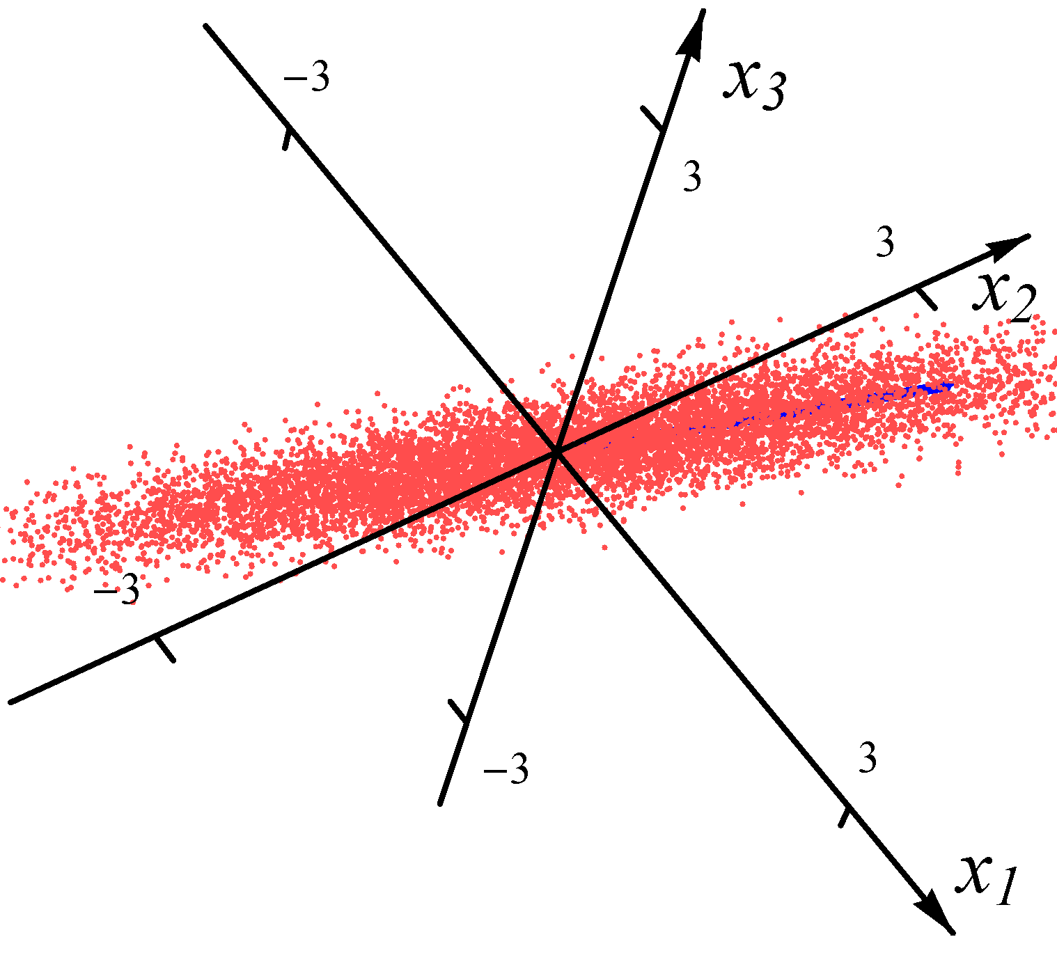
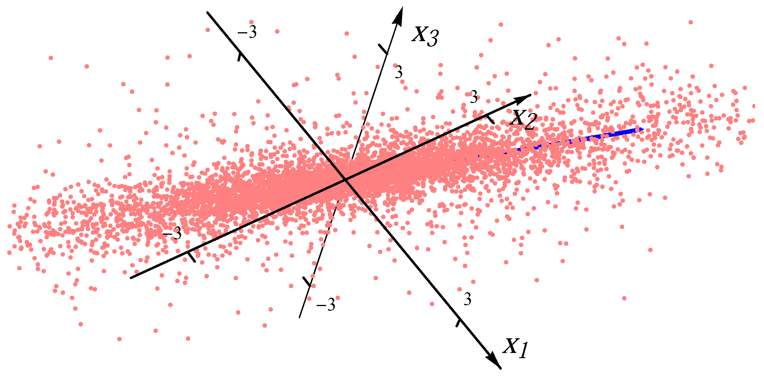
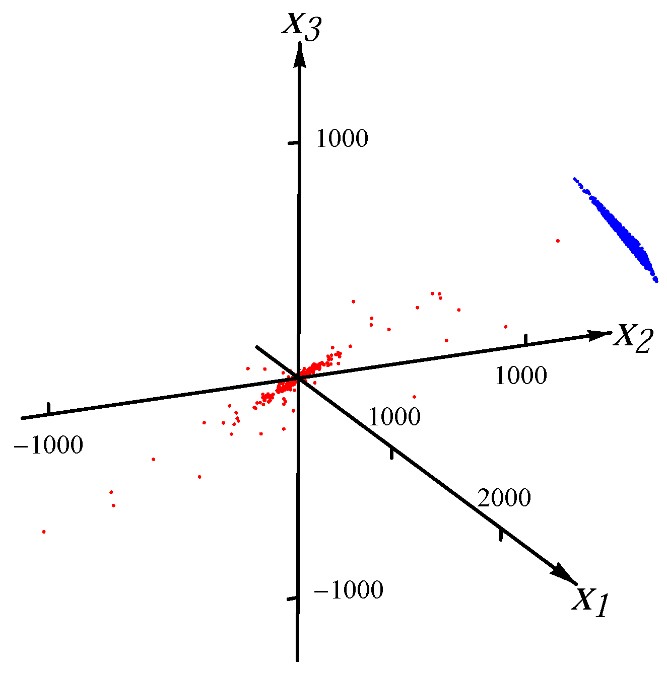
 Figure 1 and Figure 2, we present the examples of the datasets with 8000 data points (red dots) for one Gaussian distribution and one Student t distribution, respectively. In order to exhibit the major component clearly, the plot range in Figure 2 is the same as the one in Figure 1. There are many points outside the plot range of Figure 2. The directions and magnitudes of median radii in the major directions are indicated by blue bars emanating from the origin.
Figure 1. Sample from one Gaussian distribution.
Algorithms 07 00429 g001
Figure 2. Sample from one Student t distribution.
Algorithms 07 00429 g002
For the four-major-directions situation, we overlaid four distributions rotated to the directions ( 1 n , 1 n , , 1 n ) T , ( 1 , 0 , 0 , , 0 ) T , ( 0 , 1 , 0 , , 0 ) T and ( 0 , 0 , 1 , , 0 ) T . The samples for each major direction are first generated with correlation/covariance matrix σ ( n ) , and then rotated in 2 -norm to other major directions after multiplying by a factor (to make the lengths of the “spokes” different from each other). For example, for the 3D four-major-directions distribution created by overlaying four Gaussians, the median radii of the four major directions are 2.643, 3.964, 1.586 and 7.928. Figure 3 and Figure 4 show the examples of the datasets with 32,000 data points (red dots) for four superimposed Gaussian distributions and four Student t distributions, respectively. The blue bars indicate the major directions and the magnitudes of median radii in the major directions.
Figure 3. Sample from four overlaid Gaussian distributions.
Algorithms 07 00429 g003
Figure 4. Sample from four overlaid Student t distributions.
Algorithms 07 00429 g004
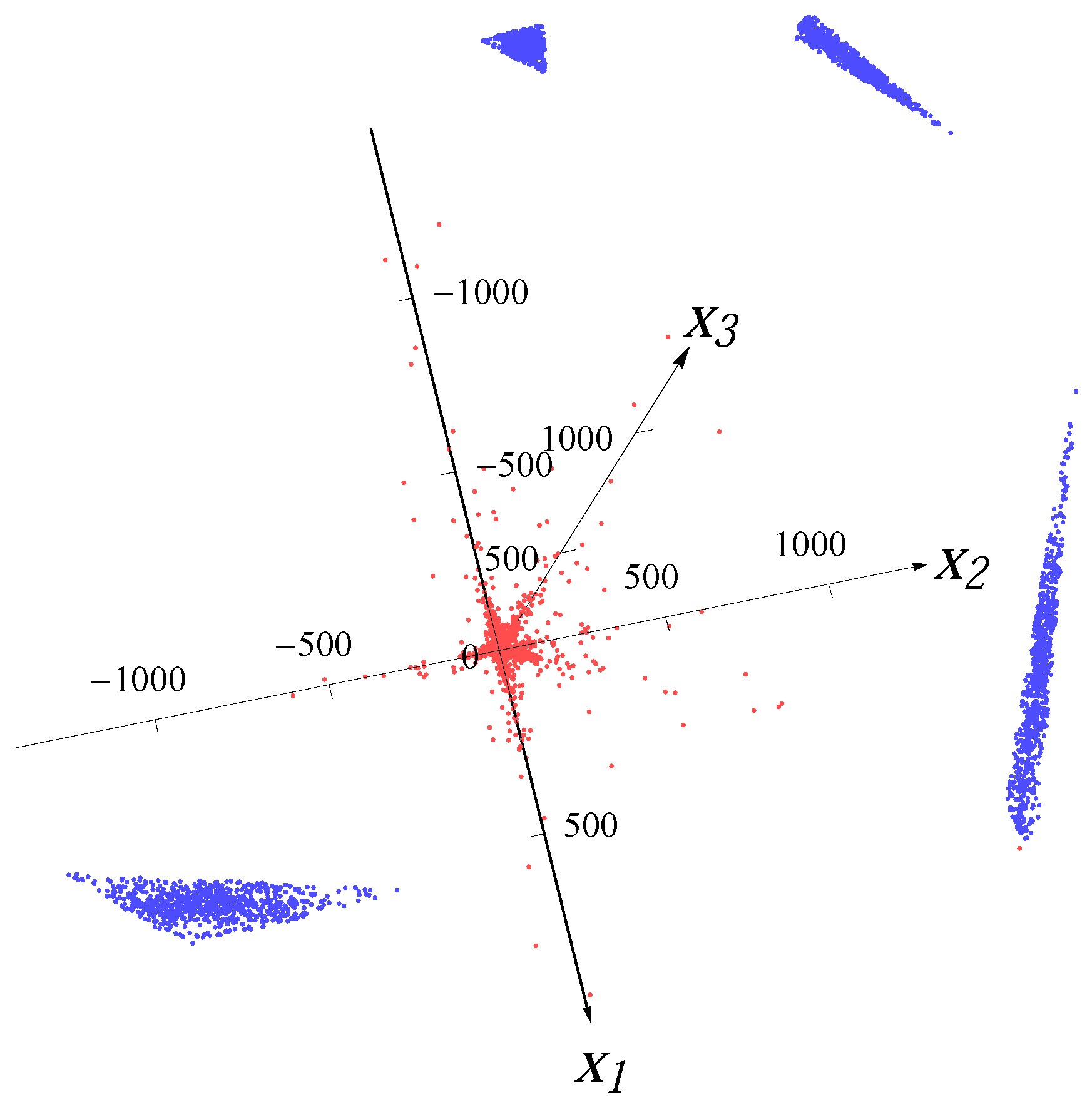
The artificial outliers are generated from a uniform distribution on a simplex. The n vertices of the simplex are randomly chosen from the intersection of the ball x 1 2 + x 2 2 + + x n 2 = 1500 2 with the hyperplane a 1 x 1 + a 2 x 2 + + a n x n = 1000 . For each distribution in the data, the angle between the normal of the hyperplane ( a 1 , a 2 , , a n ) T and the major direction of the distribution is 45 . In Figure 5, Figure 6, Figure 7 and Figure 8, we present examples with 10% artificial outliers (depicted by blue dots) for one Gaussian distribution, one Student t distribution, four superimposed Gaussian distributions and four superimposed Student t distributions (points from distributions depicted by red dots), respectively.
Figure 5. Sample from one Gaussian distribution with 10% artificial outliers.
Algorithms 07 00429 g005
Figure 6. Sample from one Student t distribution with 10% artificial outliers.
Algorithms 07 00429 g006
Figure 7. Sample from four Gaussian distributions with 10% artificial outliers.
Algorithms 07 00429 g007
Figure 8. Sample from four Student t distributions with 10% artificial outliers.
Algorithms 07 00429 g008
For each type of data, we carried out 100 computational experiments, each time with a new sample from the statistical distribution(s), including the uniform distributions that generated the outliers. The neighbors required in Steps 4 and 6 of the proposed 1 MCDA were calculated by the k-nearest-neighbors (kNN) method [20]. Other methods for identifying neighbors may also be used.
To measure the accuracy of the results, we calculated the average over 100 computational experiments of the absolute error of each major direction and the average of the relative error of the median radius in that direction vs. the theoretical values of the direction of maximum spread and the median radius in that direction of the distribution. The theoretical value of major direction for the one-major-direction case is ( 1 / n , , 1 / n ) T and the theoretical values of major directions for the four-major-directions case are ( 1 / n , , 1 / n ) T , ( 1 , 0 , , 0 ) T , ( 0 , 1 , 0 , , 0 ) T , ( 0 , 0 , 1 , 0 , , 0 ) T , respectively. The theoretical value of median radius for each major direction is calculated as the value of r * such that 0 r * f ( r | θ ) d r / 0 + f ( r | θ ) d r = 0 . 5 by numerical integration, where f ( r | θ ) is the conditional probability density function of radius r along the major direction θ.
In Table 1, Table 2, Table 3 and Table 4, we present computational results for the sets of 8000 points with local neighborhood of size I = 160 (2% of total points) for the one-major-direction situation. We compared our method with the methods that appeared in the literature [5,17]. Specifically, the MATLAB version of pcaPP [21] package of the R language for statistical computing [22] was used to implement the robust PCA proposed by Croux and Ruiz-Gazen in [5]. Brooks et al.’s L 1 PCA [17] was implemented by using MATLAB and IBM ILOG CPLEX 12.5 [23]. The computational results for those two PCA methods are also summarized in Table 1, Table 2, Table 3 and Table 4. Table 5 shows the average computational time for each method when n = 10 . For higher dimensions, the average computational time of 1 MCDA is shorter than the other two PCA methods. In Table 6, Table 7, Table 8 and Table 9, we present the computational results for 32,000 points with local neighborhood of size I = 320 , 160 and 80 (i.e., 2%, 1% and 0.5% of total points, respectively) for the four-major-directions situation.
Table 1. The results of 1 MCDA and Robust PCAs on one Gaussian distribution.
n 1 MCDACroux + Ruiz-GazenBrooks et al.
av. abs_err of angleav. rel_err ra. of lengthav. abs_err of angleav. rel_err ra. of lengthav. abs_err of angleav. rel_err ra. of length
30.01120.03140.02890.06810.05560.0675
80.02330.24980.03990.21770.01180.1586
100.02770.31290.03080.26830.00900.2256
300.03150.57720.01120.53080.00520.5099
500.03630.65390.01360.6269
Table 2. The results of 1 MCDA and Robust PCAs on one Student t distribution.
n 1 MCDACroux + Ruiz-GazenBrooks et al.
av. abs_err of angleav. rel_err ra. of lengthav. abs_err of angleav. rel_err ra. of lengthav. abs_err of angleav. rel_err ra. of length
30.02760.09210.03460.12240.05570.1310
80.04230.20350.04830.21130.01180.1800
100.04410.27170.04550.26250.00900.2352
300.04460.53670.01130.51630.00530.4869
500.04480.63500.01400.6100
Table 3. The results of 1 MCDA and Robust PCAs for one Gaussian distribution with 10% artificial outliers.
n 1 MCDACroux + Ruiz-GazenBrooks et al.
av. abs_err of angleav. rel_err ra. of lengthav. abs_err of angleav. rel_err ra. of lengthav. abs_err of angleav. rel_err ra. of length
30.01190.03730.03180.07590.05600.0654
80.02360.25120.04990.22920.02110.1588
100.02790.31340.05490.27810.01700.2289
300.03220.57850.09900.53760.00720.5077
500.03750.66010.13930.6308
Table 4. The results of 1 MCDA and Robust PCAs for one Student t distribution with 10% artificial outliers.
n 1 MCDACroux + Ruiz-GazenBrooks et al.
av. abs_err of angleav. rel_err ra. of lengthav. abs_err of angleav. rel_err ra. of lengthav. abs_err of angleav. rel_err ra. of length
30.02760.09690.03660.11400.05540.1515
80.04240.20380.05560.20540.02140.1714
100.04410.27250.06160.27750.01700.2314
300.04670.53760.10090.52380.00720.4833
500.04490.63510.13900.6142
Table 5. Average computational times (in seconds) to generate the results in Table 1, Table 2, Table 3 and Table 4 for n = 10 .
1 MCDACroux + Ruiz-GazenBrooks et al.
Table 13.774.20236.03
Table 23.644.50239.32
Table 33.554.46286.29
Table 43.214.49278.69
Table 6. The results of 1 MCDA on four superimposed Gaussian distributions.
nknn = 640 (2%)knn = 320 (1%)knn = 160 (0.5%)
av. abs_err of angleav. rel_err ra. of lengthav. abs_err of angleav. rel_err ra. of lengthav. abs_err of angleav. rel_err ra. of length
30.01240.04990.00890.03740.01210.0428
100.02260.09040.02940.06660.03640.0805
500.02690.53230.03520.49310.04480.4518
Table 7. The results of 1 MCDA on four superimposed Student t distributions.
nknn = 640 (2%)knn = 320 (1%)knn = 160 (0.5%)
av. abs_err of angleav. rel_err ra. of lengthav. abs_err of angleav. rel_err ra. of lengthav. abs_err of angleav. rel_err ra. of length
30.01200.05520.01550.07940.02110.1420
100.02250.32250.03180.24580.04370.1777
500.02500.62200.03350.58140.04300.5355
Table 8. The results of 1 MCDA on four superimposed Gaussian distributions with 10% artificial outliers.
nknn = 640 (2%)knn = 320 (1%)knn = 160 (0.5%)
av. abs_err of angleav. rel_err ra. of lengthav. abs_err of angleav. rel_err ra. of lengthav. abs_err of angleav. rel_err ra. of length
30.01520.03960.00990.04060.01710.0493
100.02710.26140.02080.30440.01730.3615
500.03790.62750.03080.65660.02610.6920
Table 9. The results of 1 MCDA on four superimposed Student t distributions with 10% artificial outliers.
nknn = 640 (2%)knn = 320 (1%)knn = 160 (0.5%)
av. abs_err of angleav. rel_err ra. of lengthav. abs_err of angleav. rel_err ra. of lengthav. abs_err of angleav. rel_err ra. of length
30.02790.16390.01840.09410.01730.0501
100.04520.16710.03360.25700.02380.3308
500.04990.53330.03880.58510.02930.6198
Remark 3. In Table 1, Table 2, Table 3 and Table 4, the radius information for the robust PCA methods [5,17] was generated by Step 6 of the algorithm described in this paper with the major directions returned by their own. Some results are not available because the computational time exceeded the limit of 3600 s.
Remark 4. In Table 6, Table 7, Table 8 and Table 9, no results for either Croux and Ruiz-Gazen’s robust PCA or Brooks et al.’s L 1 PCA are presented, because these two methods provide only one major direction for the superimposed distributions and do not yield any meaningful information about the individual major direction.
The results in Table 1 and Table 2 indicate that, when there is only one major direction in the data, 1 MCDA obtains comparable results to Croux and Ruiz-Gazen’s robust PCA in accuracy. Although Brooks et al.’s L 1 PCA outperforms the proposed 1 MCDA, it requires much longer computational time as shown in Table 5. The results in Table 3 and Table 4 indicate that 1 MCDA outperforms Croux and Ruiz-Gazen’s robust PCA in all cases, especially when the dimension is larger than 30. Brooks et al.’s L 1 PCA obtained similar results as 1 MCDA but consumed much more CPU time as shown in Table 5. It is noticeable that the accuracy of the proposed method decreases as the dimension increases. The reason is that for a given data size, the number of points falling into a fixed neighbor of the major direction decreases and the two-level median estimation deteriorates as the dimension grows higher. In contrast, the accuracy of the robust PCAs increases as the dimension increases because both robust PCAs used project-pursuit method, whose performance degrades when the underlying dimension decreases [17].
The results in Table 6, Table 7, Table 8 and Table 9 indicate that our method can obtain good accuracy by using a small neighbor size (up to 2% of the size of given data) for the four-major-directions case. It is worth to point out that the four major directions are not orthogonal to each other, and the proposed 1 MCDA is very robust by noting that the accuracy of 1 MCDA for data with the artificial outliers is as good as the one of 1 MCDA without outliers. Although the distributions designed in the experiment are symmetrically around some center, the proposed algorithm can also deal with the data from asymmetric distributions.
The computational results show that, for the types of data considered here, 1 MCDA has the marked advantage in accuracy and efficiency when comparing with robust PCAs. Moreover, 1 MCDA can deal with cases of multiple components for which standard and robust PCAs perform less well or even poorly.

4. Conclusions and Future Work

The assumptions of the distribution underlying 1 MCDA are much less restrictive than those underlying most robust PCAs. The 1 MCDA that we have developed has the following advantages: (1) it allows use of various distance functions in the data space (although we used 2 norm in this paper); (2) it works well for both heavy-tailed and light-tailed distributions; (3) it is applicable to data that have multiple spokes, contain patterned outliers, and do not necessarily have mutually orthogonal major directions; (4) it does not require the assumption of sparsity of the major components or of the error, and (5) it utilizes local information, instead of global information, in each iteration to improve the efficiency. These advantages allow 1 MCDA to be used in many circumstances in which robust PCAs cannot be used. For many geometric problems and for, perhaps, most “soft” problems (face and pattern recognition, image analysis, social network analysis, etc.), irregularly positioned “spokes” with many outliers are likely to be commonly encountered. Identifying these spokes is part of a process of generating semantics from raw data. With the ability to recover complex spoke structures in spite of the presence of heavy-tailed statistical noise and of clutter, 1 MCDA shows its potential to generate better semantics from data than other methods.
Topics that require further investigation include:
  • Use of alternative principles for calculation of the central point (for example, for V-shaped distributions or more complicated asymmetric distributions with spokes for which the median of the data is not a meaningful central point);
  • Properties of 1 MCDA for high dimensions ( 10 4 to 10 6 );
  • Ability of 1 MCDA to deal with missing data.
Irregular, high-dimensional heavy-tailed distributions are likely to describe a large number of financial, economic, social, networking, and physical phenomena. The 1 MCDA proposed in this paper is a candidate for a new, fully robust procedure that can be used for going from data to semantics for such phenomena.

Acknowledgments

This work was generously supported by United States Army Research Office Grant # W911NF-04-D-0003, by the North Carolina State University Edward P. Fitts Fellowship and by United States National Science Foundation Grant # DMI-0553310. It is the policy of the Army Research Office (ARO) that university personnel do not need to do joint work with ARO personnel in order to receive grants from ARO. We also thank to the two anonymous reviewers whose comments improved the quality of this paper.

Author Contributions

The authors contributed equally to this paper.

Conflicts of Interest

The authors declare no conflict of interest.

References

  1. Jolliffe, I.T. Principal Component Analysis, 2nd ed.; Springer: New York City, NY, USA, 2002. [Google Scholar]
  2. Candès, E.J.; Li, X.; Ma, Y.; Wright, J. Robust Principal Component Analysis; Technical Report No. 13; Department of Statistics, Stanford University: Stanford, CA, USA, 2009. [Google Scholar]
  3. Choulakian, V. L1-Norm projection pursuit principal component analysis. Comput. Stat. Data Anal. 2006, 50, 1441–1451. [Google Scholar] [CrossRef]
  4. Croux, C.; Filzmoser, P.; Fritz, H. Robust sparse principal component analysis. Technometrics 2013, 55, 202–214. [Google Scholar] [CrossRef]
  5. Croux, C.; Ruiz-Gazen, A. High breakdown estimators for principal components: The projection-pursuit approach revisited. J. Multivar. Anal. 2005, 95, 206–226. [Google Scholar] [CrossRef]
  6. Ke, Q.; Kanade, T. Robust L1 norm factorization in the presence of outliers and missing data by alternative convex programming. IEEE Conf. Comput. Vis. Pattern Recognit. 2005, 1, 739–746. [Google Scholar]
  7. Kwak, N. Principal component analysis based on L1-norm maximization. IEEE Trans. Pattern Anal. 2008, 30, 1672–1680. [Google Scholar] [CrossRef] [PubMed]
  8. Lin, Z.; Chen, M.; Wu, L.; Ma, Y. The Augmented Lagrange Multiplier Method for Exact Recovery of Corrupted Low-Rank Matrix. Available online: http://arxiv.org/abs/1009.5055 (accessed on 18 October 2013).
  9. Xu, H.; Caramanis, C.; Mannor, S. Outlier-robust PCA: the high-dimensional case. IEEE Trans. Inf. Theory 2013, 59, 546–572. [Google Scholar] [CrossRef]
  10. Gribonval, R.; Nielsen, M. Sparse approximations in signal and image processing. Signal Process. 2006, 86, 415–416. [Google Scholar] [CrossRef] [Green Version]
  11. Lai, M.-J.; Wang, J. An unconstrained q minimization with 0 < q ≤ 1 for sparse solution of under-determined linear systems. SIAM J. Optim. 2010, 21, 82–101. [Google Scholar]
  12. Candès, E.J.; Wakin, M.B. An introduction to compressive sampling. IEEE Signal Process. Mag. 2008, 25, 21–30. [Google Scholar] [CrossRef]
  13. Chartrand, R. Exact reconstruction of sparse signals via nonconvex minimization. IEEE Signal Process. Lett. 2007, 14, 707–710. [Google Scholar] [CrossRef]
  14. Auquiert, P.; Gibaru, O.; Nyiri, E. Fast L 1 k C k polynomial spline interpolation algorithm with shape-preserving properties. Comput. Aided Geom. Des. 2011, 28, 65–74. [Google Scholar]
  15. Yu, L.; Jin, Q.; Lavery, J.E.; Fang, S.-C. Univariate cubic L1 interpolating splines: Spline functional, window size and analysis-based algorithm. Algorithms 2010, 3, 311–328. [Google Scholar] [CrossRef]
  16. Tian, Y.; Jin, Q.; Lavery, J.E.; Fang, S.-C. 1 major component detection and analysis (1 MCDA): Foundations in two dimensions. Algorithms 2013, 6, 12–28. [Google Scholar] [CrossRef]
  17. Brooks, J.P.; Dulá, J.H.; Boone, E.L. A pure L1-norm principal component analysis. Comput. Stat. Data Anal. 2013, 61, 83–98. [Google Scholar] [CrossRef] [PubMed]
  18. Deng, Z.; Luo, J. FANGroup-Fuzzy And Neural Group at North Carolina State University. Available online: http://www.ise.ncsu.edu/fangroup/index.htm (accessed on 8 August 2014).
  19. MATLAB Release 2012a; The MathWorks Inc.: Natick, MA, USA, 2012.
  20. Friedman, J.H.; Bentely, J.; Finkel, R.A. An algorithm for finding best matches in logarithmic expected time. ACM Trans. Math. Softw. 1997, 3, 209–226. [Google Scholar] [CrossRef]
  21. Filzmozer, P.; Fritz, H.; Kalcher, K. pcaPP: Robust PCA by Projection Pursuit. Available online: http://cran.r-project.org/web/packages/pcaPP/index.html (accessed on 22 March 2013).
  22. R Development Core Team. R: A Language and Environment for Statistical Computing; R Foundation for Statistical Computing: Vienna, Austria, 2011. [Google Scholar]
  23. IBM ILOG CPLEX Optimization. Available online: http://www-01.ibm.com/software/commerce/ optimization/cplex-optimizer/ (accessed on 16 March 2014).

