Article

A Practical and Robust Execution Time-Frame Procedure for the Multi-Mode Resource-Constrained Project Scheduling Problem with Minimal and Maximal Time Lags

1
Department of Marketing and Distribution Management, Nanya Institute of Technology, Taoyuan 32091, Taiwan
2
Department of Industrial Engineering and Management, Yuan Ze University, Taoyuan 32003, Taiwan
3
Innovation Center for Big Data and Digital Convergence, Yuan Ze University, Taoyuan 32003, Taiwan
*
Author to whom correspondence should be addressed.
Algorithms 2016, 9(4), 63; https://doi.org/10.3390/a9040063
Submission received: 4 July 2016 / Revised: 6 September 2016 / Accepted: 16 September 2016 / Published: 24 September 2016
(This article belongs to the Special Issue Metaheuristic Algorithms in Optimization and Applications)

Abstract

:
Modeling and optimizing organizational processes, such as the one represented by the Resource-Constrained Project Scheduling Problem (RCPSP), improve outcomes. Based on assumptions and simplification, this model tackles the allocation of resources so that organizations can continue to generate profits and reinvest in future growth. Nonetheless, despite all of the research dedicated to solving the RCPSP and its multi-mode variations, there is no standardized procedure that can guide project management practitioners in their scheduling tasks. This is mainly because many of the proposed approaches are either based on unrealistic/oversimplified scenarios or they propose solution procedures not easily applicable or even feasible in real-life situations. In this study, we solve a more true-to-life and complex model, Multimode RCPSP with minimal and maximal time lags (MRCPSP/max). The complexity of the model solved is presented, and the practicality of the proposed approach is justified depending on only information that is available for every project regardless of its industrial context. The results confirm that it is possible to determine a robust makespan and to calculate an execution time-frame with gaps lower than 11% between their lower and upper bounds. In addition, in many instances, the solved lower bound obtained was equal to the best-known optimum.

1. Introduction

The main objective of researchers should be to develop methods that expand the industrial state-of-the-art in order to increase productivity, reduce costs or overall improve the performance measures. However, these methods must not only be theoretically possible based on models, but must also be robust, practical and easy to implement for practitioners. In many cases, however, researchers’ models are oversimplified and do not reflect the actual conditions faced by practitioners. Other times, the proposed solutions are too difficult to implement in real-life situations. This paper examines one such example, the Resource-Constrained Project Scheduling Problem (RCPSP), which is found in practically every industry and has long been a focus of interest among the operations research community. However, despite the high level of interest, no standard framework has emerged to guide practitioners in creating a project schedule that allocates limited resources in such a way as to: (1) maximize outcomes; (2) minimize risks of delay or failure; (3) ensure adherence to budgets and schedules; (4) ensure that quality meets expectations; and (5) eliminate the scheduler’s experience as an impact factor.
Taking these factors into consideration, in a previous study, the authors proposed a methodology to develop robust, upper-bounded schedules for the Multi-mode RCPSP (MRCPSP), a more realistic variation of the RCPSP. In this paper, however, the methodology is extended to a considerably more complicated and true-to-life model, the MRCPSP with minimal and maximal time lags (MRCPSP/max). The most significant difference between these two models is that, due to its constraints, the MRCPSP/max presents loops between activities. This means that an activity i can be both a predecessor and a successor of an activity j. Not only does this condition make the problem more difficult to solve, but it also resembles a real-life situation, which is not accounted for in the MRCPSP model. On the other hand, the methodology used only requires inputs that should be included in every project, i.e., estimations of activity durations and the set of precedencies that need to be satisfied. The proposed methodology results in execution time-frames, meaning a makespan range (minimum and maximum makespan) in which a project can be executed. These schedule execution time-frames usually include the benchmark’s best-known solution, as the lower bound and the upper bounds are on average no larger than 11% of their own lower bound. The rest of this article is organized as follows: Section 2 presents a literature review for the characteristics of past models and the solutions proposed in other studies; Section 3 details the proposed methodology; Section 4 summarizes the results, and conclusions are presented in Section 5.

2. Literature Review

Project managers in every industry seek to devise schedules that allow the efficient allocation of limited resources. These schedules are only predictive, and yet, to be applicable in practice, they should be capable of withstanding variations. Thus, the challenge is to minimize a project’s makespan, while fully satisfying all of its constraints, including enough buffer time to handle variations, but not so much as to make it infeasible. Past efforts to address this issue have produced different models, proposed different objective functions and created an array of solution procedures that help practitioners partially achieve their scheduling goals. In this section, some of the RCPSP variations, the objective functions solved and solution procedures proposed are introduced. Two fundamental concepts for the proposed approach are also discussed.

2.1. The RCPSP and Its Variations

2.1.1. RCPSP

In an oversimplified manner, a project consists of completing a set of tasks, usually in the shortest possible time, while following established precedence relationships. Techniques like the Critical Path Method (CPM) and the Program Evaluation and Review Technique (PERT) are easily applicable when the only constraint is to follow the precedence relations. However executing tasks usually require resources that are available in limited amounts; some of them renew through periods of time, and some are only available once throughout the duration of the project. When these two constraints are included (precedence and resource availability) and each task can be executed in the only way, the scheduling problem is known as the Resource-Constrained Project Scheduling Problem (RCPSP). The RCPSP has been thoroughly studied, and it has been proven to be non-deterministic polynomial-time hard, NP-hard in [1].
In reality, nevertheless, seldom can tasks be completed in only one way. A more realistic situation is that in which there are different alternatives in which a task can be completed. Ideally, every alternative leads to a different duration and requires different resources and/or amounts of resources. This is a generalization of the RCPSP known as the Multi-mode Resource-Constrained Project Scheduling Problem (MRCPSP), and Kolish proved the NP-hardness of the MRCPSP as a generalization of the RCPSP in [2].

2.1.2. MRCPSP

Though practical as an initial model, the RCPSP oversimplifies what practitioners face in reality. Therefore, Elmaghraby introduced the concept of modes to represent the different alternatives in which an activity can be executed [3]. These modes resemble real-life scenarios where an activity can be executed faster (at greater resource expense) or slower (and hopefully more economically), depending on the project manager’s preference and/or the overall project status.
A second characteristic of real-life projects is the inclusion of non-renewable resources. These are fixed resources (e.g., capital budgets) that (should) extend throughout the project’s duration and which cannot be replenished once consumed. These two characteristics, along with those already considered in RCPSP (i.e., precedence constraints, no-preemption, renewable resources, etc.), define the multi-mode resource-constrained project scheduling problem, a generalization of the RCPSP.
Some of the variations of the MRCPSP include a real-life situation that is commonly executed when the project is running behind schedule to significantly shorten the activity duration at the expense of additional cost. This was modeled by the use of special modes called “crashable modes”, introduced in [4]. A situation in which some activities require personnel with certain skill levels was modeled and solved in [5]. Additionally, among others, Zu et al. examined a variation of MRCPSP with generalized resource constraints in [6], while Heilmann, Nonobe and Ibaraki examined precedence constraints in [7,8,9], respectively.

2.1.3. MRCPSP/Max

One of the MRCPSP constraints states that the successor of an activity i can only be an activity j whose index is greater than that of i. The effect of this constraint is that the project can only advance linearly; thus, there is no way in which an activity j can return to a previously-done activity i. This constraint limits the representation of situations in which an intermediate activity (e.g., a quality inspection) must be completed before the current activity can be declared as completed.
Another MRCPSP limitation is that there is no way to specify the time lag (if any) between activities. In real-life situations, practitioners sometimes will sometimes need to delay the beginning of an activity depending on how the activity that is currently ongoing is executed. This is represented by the use of weights on arcs connecting the modes between different activities. Translated to a real-life scenario, these weights can be thought of as “penalties” for particular execution modes imposed by the scheduler probably based on soft constraints.
These characteristics distinguish the MRCPSP with minimal and maximal time lags (MRCPSP/max) from other variations of the MRCPSP. The MRCPSP/max has been studied, though not as extensively as the single-mode problem with time lags (see [7,8]). Furthermore, one variation where time lags depend on the mode chosen can be found in [10]. Section 3 will detail the mathematical formulation and an example for the MRCPSP/max.

2.2. Objectives Solved and Solution Procedures

Though the most solved objective functions for the MRCPSP and its variations are concerned with the minimization of makespan Kolisch and Padman [11], other performance indicators have also been considered. Some researchers have examined time performance indicators, such as the components of lateness, Lj, and the deviation of an activity’s completion time (Cj) from a given due date (dj). Tardiness (Tj), the positive value of lateness (Cj ≥ dj) and earliness (Ej), the negative value of lateness (Cj ≤ dj), have been researched within the last 15 years by [12].
Other researchers have focused on financial performance indicators, such as activity and total project costs. For example, Möhring and Schulz [13,14] and Nonobe and Ibaraki [9] minimized the costs of activities, while Achuthan and Hardjawidjaja [15] minimized the total project costs based on earliness and tardiness costs, as well as Dodin and Elimam [16] aimed at minimizing costs for activity crashing, material costs and inventory holding costs. Another financial indicator used as an objective function is the maximization of the Net Present Value (NPV), including [17,18]. In [19], they investigated the negotiation process to find the timing of payments and the amount of each specific payment between a client (who seeks to minimize its NPV) and a contractor (seeks to maximize NPV). Furthermore, variations of NPV objective functions can be found in [20]. Dayanand and Padman [21] treated a similar problem, but restricted themselves to the client’s point of view.
Thanks to significant improvements in computing power and as increased complexity highlights the limitations of exact methods, many researchers have opted to use time-proven meta-heuristic algorithms to solve the MRCPSP and its variations. Some meta-heuristic algorithms used with the last two decades include two versions of the Simulated Annealing (SA) algorithm by [22], a version of the Genetic Algorithm (GA) developed by [23]. Other approaches include Particle Swarm Optimization (PSO) by [24] and a combinatorial version for PSO in [25]. Furthermore, many hybrid forms have been implemented, such as a scatter search algorithm with a path re-linking methodology in [26], a hybrid Ant Colony Optimization and Scatter Search (ACOSS) in [27], a Tabu Search (TS) with scatter search implemented by [28], as well as a neuro-genetic approach, which is a hybrid of GA and a neural network, proposed by [29], and more recently, ANGEL, a hybrid that combines ANt colony, GEnetic algorithm and Local search can be found in [30]. Finally, the newest meta-heuristic implementations can be found, including Differential Evolution (DE) [31], Artificial Immune System (AIS) [32] and, most recently, Estimation of Distribution Algorithm (EDA) [33], the shuffled frog-leaping algorithm (SFLA) [34], a hybrid EDA with a new local search based on a random walk and the delete-then-insert operator proposed by [35] along with the use of a discrete version of the ABC algorithm in [36] and an implementation of a discrete cuckoo search in [37].

2.3. Measuring Uncertainty

Given that project execution is always subject to some degree of uncertainty, much research has been dedicated to the generation of buffer times to handle eventualities. All of these models present different advantages, but nearly all present a major drawback in that they are subject to the extent of the scheduler’s experience. One of the most widely-used approaches is fuzzy systems, which is especially well-suited to handle vague information. Long and Osato [38] proposed a fuzzy critical chain method, which developed a desirable deterministic schedule under resource constraints and added a project buffer to the end of the schedule to deal with uncertainty. In an attempt to handle uncertainty in activity duration, Chen et al. [39] used fuzzy set theory to represent the uncertainties of activity duration. Meanwhile, Xu et al. [40] presented a bi-level model for project scheduling in a fuzzy random environment.
Stochasticity presents a different approach to handle uncertainty. Rabbani et al. [41] developed a technique for stochastic network resource allocation decisions with imprecise durations for each activity; Larrañaga and Lozano [42] used the Estimation of Distribution Algorithm (EDA), a kind of stochastic optimization algorithm based on statistical learning; and most recently, Hao et al. [43] proposed a multi-objective Estimation Distribution Algorithm (moEDA) to minimize a schedule’s robustness and expected makespan.
The approach presented here uses the concept of entropy, a key term in thermodynamics, which does not depend on the scheduler’s experience. In [44], Bushuyev and Sochnev formulated a way to measure activity entropy as shown in Equation (1), with complete project entropy calculated using Equation (2). Ei, represents the set of unfavorable events for activity i. The value δt is a relevant time interval and is dependent on the nature of the project in the sense that its value is negatively correlated to the level of project risk. From a practitioner’s point of view, we can think of δt as checkpoints or meetings in which the project manager receives updated project status information. The higher the risk of a schedule disruption, the more control needs to be exerted, requiring more frequent updates. For this study, we fixed the value of δt = 1 based on a sensitivity analysis performed in our previous research. The slack, si, is determined by the standard forward (backward) recursion procedure. The values diu, di and dil respectively stand for the longest, most probable and shortest possible durations, while EFT and LFT respectively represent the earliest and latest finish times with the corresponding durations indexed. Ei results as the time difference between L F T d i and E F T d i u , as shown in Equation (3).
S I D =   E i ( d i u d i l ) ln ( δ t d i u d i l )    
S =   I D S I D  
E i = ( d i u d i ) s i =   E F T d i u L F T d i  
From these equations, one can see that an activity’s entropy depends solely on the range of the estimation for its duration, i.e., the larger the difference between diu, di and dil, the more uncertain the scheduler considers the activity to be, and thus, the higher the value of its entropy. Figure 1 gives a graphical representation of Ei and δt. Here, the solid grey bar represents an activity scheduled with a most probable duration di, and slack, si, is the time interval between E F T d i and L F T d i . The white bar shows the E F T d i l and E F T d i u ; Ei represents the unfavorable events; and the relevant time interval parameter defined by the user is shown as δt.

2.4. Schedule Robustness

The term “schedule robustness” introduced by [45] is “the ability (of a schedule) to cope with small increases in the time duration of some activities that may result from incontrollable factors”. Based on this concept, Chtourou and Haouari [46] introduced a schedule robustness measure, which, in the case of excessively large slack, allows the use of the minimum value between the slack and a fraction of the activities’ duration (min(si, frac × di)). The user can define the value of frac; however, based on a sensitivity analysis performed in the authors’ previous study [36], the value of frac is fixed to 0.25 for the experiments performed in this study. Section 3 explains the use of this robustness measure in the proposed method.

3. Model and Methodology

3.1. Mathematical Formulation of MRCPSP/Max

For this section, we follow the model presented in [47]. Consider a project with n + 2 activities belonging to the set V = {0, 1, 2, …, n, n + 1} where activities 0 and n + 1 are dummies that represent the beginning and end of the project, respectively. Every activity i has to be executed in only one mode µi M out of the total available for every activity Mi = {1, …, |Mi|}. The duration of every activity, d i μ i , depends on the mode µ selected, and the beginning and end of every activity is denoted by Si and Ci correspondingly. Therefore, if activity i begins at time Si, it will continue to be executed in mode µi throughout time t = [Si, Si + d i μ i ], so if S0 := 0, then the duration of the project is given by Sn+1. Between the start times of activities i and j, a time lag p can be included. This time lag is dependent on the mode µi of activity i and µj of activity j (ij) and can be maximal p i μ i j μ j m a x or minimal p i μ i j μ j m i n .
The activities and time lags are represented by an activity-on-node network N with node set V, arc set E and arc weight function δ; N = <V, E, δ>. Every element of V represents an activity, and every element of E represents a time lag that must be observed. Arc weight function δ is a matrix defined by user preferences that assigns to each arc <i, j> a time lag as follows: for a minimum time lag δ i μ i j μ j m i n   p i μ i j μ j m i n and for a maximum time lag δ i μ i j μ j m a x   p i μ i j μ j m a x . As previously mentioned, the inclusion of such time lags leads to cycles in N that make the MRCPSP/max problem much more complex than other versions of MRCPSP.
Furthermore, every non-dummy activity i executed in mode μi consumes r i μ i k ρ type k renewable per period of time out of a total R k ρ renewable resources available in the project and r i μ i k v nonrenewable resource out of a total R k v . Dummy activities consume no resources and have duration = 0.
A schedule (M, S) consists of a mode vector M and a start time vector S. A mode vector M = (µi) assigns only one mode µ to every activity i for it to be executed. Each mode vector M has an associated project, N(M), obtained by choosing the durations, resources and time lags corresponding to the modes of M. A start time vector S = (Si) assigns to each activity i exactly one point in time t ≥ 0 as start time Si with S0 := 0.
With A(M, S, t) := {i V|Sit < Si + d} denoting the set of activities being executed at a time t for a schedule (M, S), the MRCPSP/max can be stated as follows:
M i n   S n + 1    
subject to:
S j   S i   δ i μ i j μ j         ( < i , j > E )
i A ( M , S , t ) r i μ k ρ     R k ρ         ( k R ρ ; t 0 )
i V r i μ i k v     R k v         ( k R v )
μ i   M   ( i V )
S i   0   ( i V )
S 0   = 0
The objective function stated in Equation (4) results in the makespan of an optimal schedule (M, S) that minimizes the project duration ensuring that the time lags in Equation (5) are observed while meeting the renewable and nonrenewable resource consumption requirements established in Equations (6) and (7), respectively. Please refer to Figure 2 and Table 1 for an example of MRCPSP/max.
Table 1 shows an example of an MRCPSP/max instance. Here, all of the activities (except for the dummies, 1 and 6) can be executed in one out of three modes available. The column "duration” shows the scheduler’s estimation for the shortest, most probable and longest possible duration, dil, di and d, respectively. Column R k v . shows the amount of renewable resources consumed by the activities in each of their modes. Finally, the column “arc weight” shows the time lags when going from mode μ i of activity i to mode μ j of activity j. If the activity i is succeeded by the final dummy activity, only one arc weight is needed, i.e., Activities 3, 4 and 5. Finally, notice that Activity 4 is also a precedent for Activity 2, which, as mentioned previously, could not occur in the case of the MRCPSP. This indicates that Activity 4 is a successor and predecessor of Activity 2 and exemplifies the loops that make the MRCPSP/max both more realistic and complicated to solve.

3.2. Solution Procedure

In [36], the authors introduced a methodology that determined a schedule’s makespan upper and lower bounds for the MRCPSP. In this study, this methodology is extended to the more complex MRCPSP/max. The flowchart in Figure 3 depicts a summary of the 3-stage procedure, where MS1, MS2 and MSR respectively represent the makespan for Stage 1, Stage 2 and Stage 3. The rest of Section 3 presents the details for each of the stages. First, three tools used in two of the stages are presented: a discrete version created from a powerful optimization algorithm, followed by rules that help select execution modes (mode selection rules) and rules that help prioritize the activities (activity priority rules). Finally, how these tools are integrated into the 3-stage procedure is introduced.

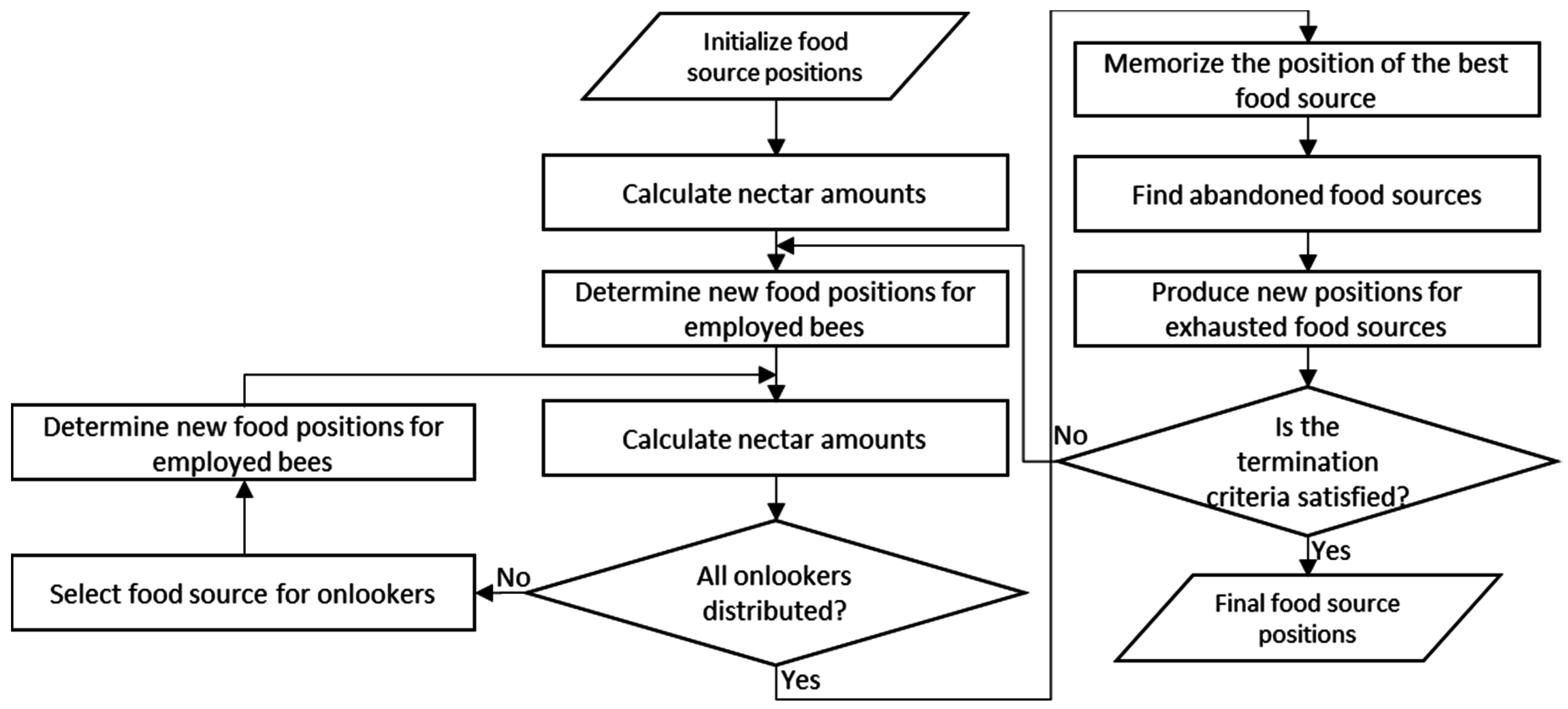
3.2.1. Discrete Artificial Bee Colony

Based on the behavior of honey bee swarms, the artificial bee colony is a population-based optimization algorithm with several distinct features that make it a good optimization tool [48]. The main idea behind it is that the search space shared by all of the bees is based on the opinion of individual bees, which are part of a society. Out of all of the groups in a colony, this algorithm considers three groups of bees: employed, onlookers and scout bees. Furthermore, in this algorithm, every solution corresponds to a food source, and the quality of each solution is associated with the amount of nectar; the higher the quality of the solution, the more nectar in that food source. The ABC algorithm incorporates the following phases:
  • Initialization: n-dimensional solutions are generated randomly throughout the search space. After the initialization phase, the algorithm is repeated a Maximum Number of Cycles (MNC), executing three improvement phases in each cycle:
  • Employed bees phase: Each solution (food source) is assigned a bee, which thus becomes an employed bee. This bee seeks to improve the solution by applying modifications (local search operators), and the quality (nectar) of the obtained solution is later compared to that of the original solution. If the modified solution is better, the old solution is forgotten, and the new solution is memorized. The employed bee will keep modifying the assigned food source until either a better solution is found or the abandonment limit is reached.
  • Onlooker bees phase: After all employed bees have finished their local search cycle, they share the nectar information of their food sources with the onlookers, each of which then selects a food source for further exploration based on the following probability:
    p i = f i i = 1 S N f i
    The onlookers tend to choose a food source i with higher probability pi among SN total food sources, each with a fitness fi.
  • Scout bees phase: If the employed and onlooker bees cannot improve a solution after a number of trials (i.e., they reach the abandonment limit), a scout bee searches for a new food source (i.e., a new solution is generated randomly), and the previous food source is abandoned.
Figure 4 shows a flowchart of the ABC algorithm. However, ABC was developed to solve continuous functions, not the current combinatorial problem. Therefore, a discrete version of the ABC algorithm is developed by representing every food source in matrix form and using the swap and insert operators for the local search. Furthermore, to increase the solution search space, the local search operators are designed to affect either only the mode of execution or the order of the activities along with their execution modes. This means that an activity list can remain unaltered, in the case that just the execution mode is selected; or it can be modified if the activity is selected; the factor affected is selected randomly. If activities are selected (i.e., activity + execution mode), a solution feasibility procedure is performed by checking the precedence constraints previous to the actual swap and/or insert. If only execution modes are selected, the activity stays in its current activity list order; the modes are swapped/inserted; and the resource constraints are checked.
Refer to Figure 5 for the following example showing how these operators work: Suppose a swap between Activities 3 and 7 results in a feasible solution; Figure 5a shows the result of this operation. If the same two activities are chosen, but only to swap their execution modes, Figure 5b shows the result. Figure 5c shows a graphical representation of inserting Activity 7 before Activity 4, and finally, Figure 5d shows the result of inserting the execution mode of Activity 7 before that of Activity 4.

3.2.2. Mode Selection Rules

One of the complexities of the MRCPSP and its variations is the multiple modes available to execute every activity. Practitioners seldom have sufficient time to simulate or even consider all of the possible outcomes of selecting different execution modes for every single activity. Instead, they focus on critical activities and deal with non-critical activities based on either intuition, experience or simple rules of thumb. In this study, five different Mode Selection Rules (MSR) are employed to determine the best execution mode for every activity based on different metrics, e.g., duration, resource consumption and combinations of these two parameters. Table 2 presents the mode selection rules used in the proposed solution procedure. The Shortest Feasible Mode (SFM) and least resources proportion were taken from [49]; the remaining three rules were taken from [50]. The mode selection rule to be used is chosen randomly, and based on this selection, the information of the mode is used to determine the activity list, resource consumption and, ultimately, the makespan of the schedule.
One critical factor to take into account when selecting modes is that given that cycles are allowed in the MRCPSP/max, the fact that the modes selected create cycles of positive length needs to be considered. A cycle of positive length is that in which the sum of the arc weights of the activities in the cycle is >0. Cycles of positive length violate the constraint in Equation (5); so, to deal with this issue, the above-mentioned MSR are used when solving the Best Mode Assignment Problem (BMAP) introduced in [47], and the approach of using a lower bound determined by the critical path is followed. Here, the authors view the MRCPSP/max as a mode assignment problem and propose to look for the best mode for each activity. The key decision variables in this model are the modes of the activities, and feasible solutions are the mode vectors that are resource and time feasible.

3.2.3. Activity Priority Rules

Once the mode for each activity is selected, the order in which the activities will be executed such that the precedence constraints are not violated needs to be determined. Similar to the way the MSR are employed to determine the modes, eleven Activity Priority Rules (APR) are used to evaluate different parameters and to determine how to prioritize the activity list. Table 3 presents the APR considered in this study:

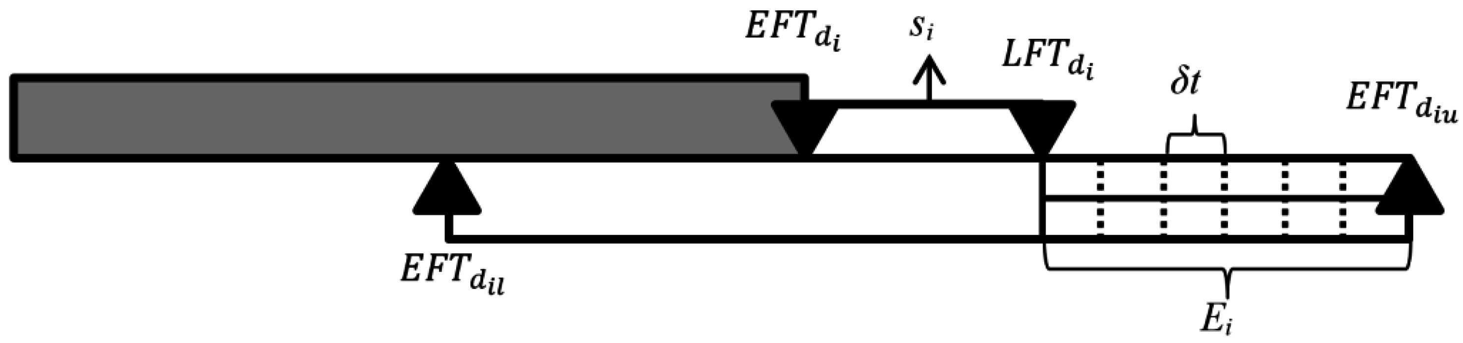
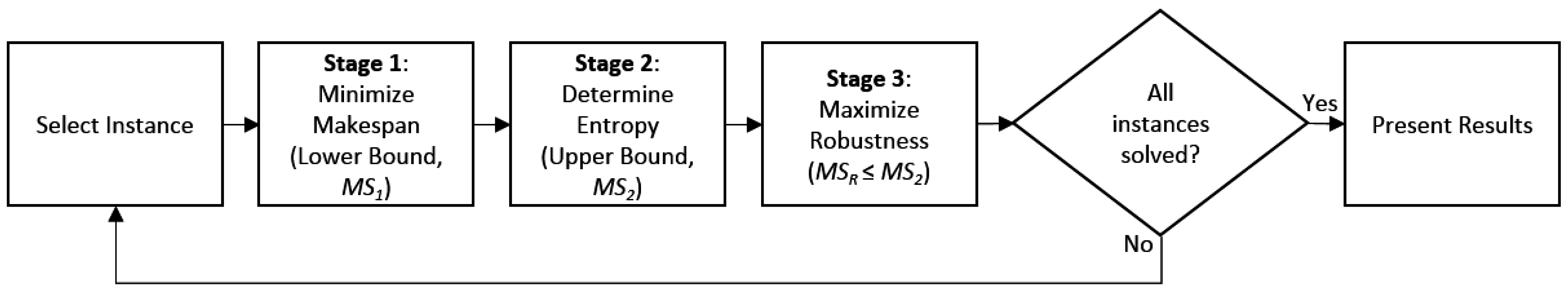
3.2.4. Three-Stage Procedure Execution Time-Frame

To determine a project’s execution time-frame, the pseudo-code Algorithm 1 is shown below, and the details is discussed in the following subsections.
Algorithm 1: Repeat until all instances are solved
  Stage 1: Minimize Makespan (Upper Bound Makespan, MS1)
   Initialization Phase
   While i < population
   Evaluate Mode Selection Rules (MSR)
   Evaluate Activity Priority Rules (APR)
  End
   Repeat until MNC
   Employed Bees Phase
   Onlooker Bees Phase
   Scout Bees Phase
  End
  Stage 2: Compute schedule’s entropy (Upper Bound Makespan)
  Stage 3: Maximize Robustness
   Initialization Phase
   While i < population
    Evaluate Mode Selection Rules (MSR)
    Evaluate Activity Priority Rules (APR)
  End
  Repeat until MNC
   Employed Bees Phase
   Onlooker Bees Phase
   Scout Bees Phase
  End
  End

Stage 1: Lower Bound Makespan

After selecting the execution modes and determining the activity list, the third step is to generate an actual schedule. Recall that schedules must be time feasible (no cycles of positive length), as well as resource feasible. A Serial Generation Scheme (SGS), which means that at every time period, only one activity is considered for scheduling, is employed. If the activity cannot be scheduled in the available time period, the time advances until the activity can be scheduled. These three steps generate one initial solution, and this procedure is repeated until the complete population (n initial solutions) has been generated; this is the initialization phase of the ABC algorithm.
In the employed bees phase, all of the solutions are selected for improvement. If a solution is not improved with the local search, a counter for solution non-improvement attempts will increase. If a solution is improved, its counter will be restarted regardless of the number of non-improvement attempts it had previously. If a solution reaches the abandonment limit for not being improved, this solution will be marked for replacement, and a new solution will be generated when the scout bees phase is reached.
The onlooker bees phase makes improvements to solutions based on the probability function described in Equation (6). With higher solution fitness, the probability for it being selected for improvement is increased. Similar to the employed bees phase, if the solution selected is not improved with the local search operators, a counter for solution non-improvement attempts will increase, but it is restarted if the solution is improved at any point. If a solution reaches the abandonment limit the solution is marked for replacement by a new solution.
The scout bees phase is the final stage in the combinatorial ABC algorithm developed. In this stage, all of the solutions that reached the abandonment limit are replaced by new solutions. These new solutions can be generated either by using the MSR detailed previously or randomly; the way in which they are determined is selected randomly. These three improvement phases are performed a maximum number of cycles times, and when this criterion is reached, the schedule with the shortest makespan is reported as the lower bound for the three-stage procedure (MS1 in Figure 3) and used as the input for Stage 2.

Stage 2: Upper Bound Makespan

Stage 2 of the proposed methodology calculates the input schedule’s entropy based solely on the precedence constraints and the three durations (shortest, most probable and longest possible duration, dil, di, and diu, respectively) estimated for every activity. Here, Equation (3) determines the set of unfavorable events, and finally, Equation (2) is used for the schedule’s total entropy. As a short example, assume there is an activity whose selected execution mode requires 7 time units. Furthermore, the scheduler determined that the activity’s most probable duration (di) was 9 time units and that the longest possible duration (diu) was 10 time units. This activity happens to be part of the critical path and, therefore, has slack s = 0. Furthermore, suppose the relevant time interval δt is set to 1. Therefore, after using Equation (2), the entropy for this activity is 1 time unit. To determine the complete schedule’s entropy, this same procedure is applied to all project activities. Nonetheless, the total time added to the current makespan is not necessarily equal to the sum of the entropy for all activities. If activities have slack greater than their entropy values, these activities will simply be shifted without affecting the overall makespan. The new entropy-containing makespan will serve as the upper bound for the execution time-frame and will also serve as an input for Stage 3 (MS2 in Figure 3).

Stage 3: Robust Makespan

The third and final stage produces a robust makespan using the result of Stages 1 and 2 as input. Even though Stages 1 and 3 both implement the discrete ABC algorithm, there are two significant differences: First, all of the initial solutions generated for Stage 3 must be within the minimized makespan of Stage 1 and the entropy-containing makespan of Stage 2 (MS1 ≤ MSR ≤ MS2 for all of the initial solutions i). Second, the objective function in Stage 3 is not to minimize the makespan, but rather to maximize the makespan’s robustness. Equation (9) shows the objective function solved in Stage 3:
M a x   Z =   m = 1 M I i = 1 I ( min ( s i μ ,   ( f r a c d i μ ) ) N s u c c i k = 1 R ρ r i μ k ρ )
where frac is a threshold (%) of activity duration (0 < frac < 1) set to 0.25 based on the authors’ previous study [36], Nsucci denotes the number of immediate successors of activity i and sim represents the slack of activity i if executed in mode μ. Equation (9) establishes that the objective is to maximize the robustness measure, which is based on the slack of each activity in each available mode.
It is worth noting that the final makespan resulting from Stage 3 cannot be larger than the makespan resulting from Stage 2, but it could be smaller than that from Stage 1. However, since the main objective is to produce a robust and practical makespan, the value of the robustness measure (RM), and not the makespan, determines if this reduced makespan will be used or not. For example, suppose a Stage 3 schedule has a makespan = 60 and RM = 140 and a Stage 1 schedule has a makespan = 62, but RM = 154. For this case, even though there is a schedule with lower makespan, 60, the selected schedule will be the one with makespan 62 because it has a higher RM. At the end of Stage 3, the schedule reported will be one with maximized robustness and with a makespan at least as low as the lower bound generated in Stage 1 and at most as high as the entropy-containing schedule generated in Stage 2.

4. Computational Results

The benchmark sets found in [58] are selected to evaluate the proposed methodology. At the moment of writing, there were three benchmark sets divided by the number of activities (30, 50 and 100 activities); each set contains 270 instances, and every instance uses three renewable, three non-renewable and three doubly-constrained resources. Furthermore, every activity can be executed in anywhere from three to five different modes, except for the dummy (initial and final) activities, which have only one mode with no duration and no resource consumption.
The experiments conducted were very straight-forward, following the procedures described in Section 3, and the only additional information used was the parameters used to evaluate the formulas, which are detailed below. The results from the methodology proposed in this study are not compared to the results of other approaches because the main objective is not to minimize makespan. The main objective for this study is introduce a procedure that generates a robust baseline schedule that lie within a lower and upper bound and which is capable of absorbing variations caused by uncertainty; to the best of the authors’ knowledge, there are no other papers that present such results. The sole point of comparison is against the best-known optima, and the results are reported based on the deviation against these Best-Known Optima (BKO). Additionally, even though the main objective was not to minimize the makespan, in most of the instances, the best-known solution was reached as the lower bound. Furthermore, the results presented are based on the schedules’ makespan, but for every makespan, there was an actual schedule (M, S) generated.

4.1. Parameters

In [36], the authors conducted a sensitivity analysis to determine the values of the parameters to be used for the ABC algorithm, as well as the entropy and robustness functions. In that study, the best results were obtained when using higher levels on parameters that increase the search space and using the lowest levels for those parameters that are linked directly to the solution’s quality. Additionally, given that this is an extension of that methodology from the MRCPSP to the MRCPSP/max, the same parameter settings developed and tested in that previous study are adopted here. It is worth noting that even though the MRCPSP and the MRCPSP/max are initially different models, the parameter setting for the solution procedure introduced is not affected because for both cases, the use of the algorithm is only after a mode vector is selected and the activity list is defined, and by this point, the same objective functions are optimized. Table 4 shows the parameter values used in this study.
With these parameters, the method is implemented as described in Section 3: in Stage 1, the discrete ABC algorithm is used to minimize the instances’ makespan (MS1); this will serve as the lower bound of the execution time-frame. In Stage 2, the entropy Equation (1) determines the upper bound (MS2). Finally, in Stage 3, the third makespan is computed also using the discrete ABC algorithm, but in this stage, seeking to maximize robustness (Equation (9)), while keeping the makespan lower than the upper bound, though not necessarily higher than the lower bound.

4.2. Results

All of the experiments were run in an Intel (Intel Corporation, Santa Clara, CA, USA) i7 personal computer with 8 GB of RAM, and the problem was coded using MATLAB R2012a. Table 5 presents summary statistics from evaluating all 270 instances of every benchmark set. Here, the Average Deviation (Avg. Dev.) is computed as the average of all of the deviations when evaluating (Ms − M*) M*, where M* represents the reference makespan when comparing the results of Stage 1 and Stage 3 (M* can be either a confirmed optimal or the Best-Known Makespan), and Ms denotes the makespan of the current stage. Furthermore, S1, S2 and BKO represent the makespan of Stage 1, Stage 2 and the Best-Known Optima (BKO), respectively.
From Table 5, it is noticed that the number of optima found decreases as the number of activities increases. This is because of the increasing complexity of the problem; however, it is worth noting that these optima can be found in two different stages (Stages 1 and 3), which explains why there can be a negative average deviation when Stage 3 is compared against Stage 1 (e.g., Column MM100) or Stage 2 (MM30 through MM100). Looking at the last column, the overall average deviation of the schedules resulting from Stage 1 is 3.06%, which confirms the power of the discrete version of the ABC algorithm implemented. Furthermore, the average deviation of the schedules resulting from Stage 2 is 9.44% when compared to the BKO, but only 5.38% when compared against the input received from Stage 1. Finally, the average deviation of the schedules resulting from Stage 3 is 4.93% when compared to the BKO, only 0.59% when compared against Stage 1 and −5.16% when compared against Stage 2.
In Table 5, the column “overall average” indicates that there is a difference between the instances’ makespan when compare against the BKO. Therefore, to test if this difference is statistically significant, Table 6 presents the hypotheses to be tested for each benchmark set, and Table 7 summaries the results.
Based on the p-values obtained for the hypotheses tested, it is concluded that there is not enough statistical evidence to reject the null hypotheses for Stage1 vs. BKO. This means that the algorithm implemented is powerful enough to reach the BKO in most of the instances tested. However, when comparing Stages 2 and 3 against the BKO, the null hypotheses are rejected, and it is concluded that the makespans for these stages are statistically larger than the BKO. This does make sense because the input for these two stages is Stage 1, and for the cases in which the BKO was not reached, it is intuitive to assume that the makespan would be larger than the BKO.
In the proposed approach, however, the focus is not on minimizing the makespan, but rather on maximizing its robustness. The minimized makespan from Stage 1 is only used as input for the entropy-containing schedule in Stage 2 and the maximized robustness schedule in Stage 3. Hence, a further analysis tests if the results for Stages 2 and 3 are statistically different from the result in Stage 1. Table 8 presents the hypotheses tested, and Table 9 shows the results.
The p-value results in Table 9 show that although the makespans obtained in Stage 3 are statistically different from the BKO, they are equal to those obtained in Stage 1 because all of the p-values obtained are greater than the significance level of 0.05. However, it is also noticed that the results obtained for Stage 2 are statistically different from the results in Stage 1, and so, a further and final analysis tests if this difference is similar to what is done among project managers in a real scenario. It is common among practitioners to add somewhat between eight and 15 percent of the budget to their final estimate in order to have a buffer time in case an uncertainty becomes a real threat. The average deviation obtained from Stage 2 against that resulting from Stage 1 is tested to see if it is lower than the lowest used by practitioners. Table 10 presents the final hypothesis tested, and Table 11 shows the results:
The results in Table 11 confirm that the proposed approach is capable of producing robust baseline schedule upper bounds that are lower than the lowest common practice followed by practitioners and which are in practically every case closer to the best know optima instead.

5. Conclusions

Taking the authors’ previous study as a reference, this research extended the methodology to a more complex and true-to-life MRCPSP/max. Unlike other studies in which the main objective is simply to minimize a project’s makespan, the objective of this study is to present a practical methodology to develop robust project execution time-frames. The main motivation for this approach emerges from the uncertainty that practitioners face in their day-to-day jobs. Regardless of the industry and the amount of planning spent on them, projects are and will always be subject to a degree of uncertainty which (foreseen or not) can not only result in delays, but also render projects infeasible.
The main factor that contributes to the proposed methodology’s practicality is the fact that it only requires inputs that are present for every project: precedence constraints and activity durations. With this input, the proposed three-stage procedure is able to determine not only a robust baseline makespan based solely on the project’s inherent entropy, but also determine a range for this makespan, or as it has been called, a project execution time-frame, because of the lower and upper boundaries generated. The main limitation of this study, however, is the lack of reference for further comparison in regards to the robustness of the makespan. Furthermore, although not included in this study, this procedure can in theory also use other optimization algorithms. As future research, the proposed procedure will be coded using other proven effective optimization algorithms and compared against the combinatorial ABC algorithm used here.

Acknowledgments

This work was partially supported by Ministry of Science and Technology in Taiwan (MOST 103-2221-E-253-005, MOST 104-2221-E-253-002) and the Innovation Center for Big Data and Digital Convergence at Yuan Ze University.

Author Contributions

All three authors contributed equally to the conception and design of the work. Angela Hsiang-Ling Chen particularly contributed her knowledge on MRCPSP/max. Yun-Chia Liang’s main contribution is the development direction of the ABC algorithm. Jose David Padilla performed the experiments and interpretation of the data, as well as drafted the article. All authors have done critical revision of the manuscript and final approval of the version together.

Conflicts of Interest

The authors declare no conflict of interest.

Abbreviations

ABCArtificial Bee Colony
ACOSSAnt Colony Optimization and Scatter Search
ACTIMActivity Time
ANGELAnt Colony and Genetic Algorithm with Local Search
APRActivity Priority Rules
BKOBest-Known Optima
BMAPBest Mode Assignment Problem
CPMDifferential Evolution
DEDifferential Evolution
EDAEstimation of Distribution Algorithm
EFTiEarliest Finish Time of activity i
GCUMRDGreatest Cumulative Resource Demand
LFTiLatest Finish Time of activity i
LNRJLeast Non-Related Jobs
LPSRDLeast Product Sum of Resource and Duration
LRPLeast Resource Proportion
LRSLeast sum of Non-renewable Resource
LTRULeast Total Resource Usage
MISMost Immediate Successors
MNCMaximum Number of Cycles
moEDAMulti-Objective Estimation Distribution Algorithm
MRCPSPMulti-mode Resource Constrained Project Scheduling Problem
MRCPSP/maxMultimode RCPSP with minimal and maximal time lags
MSiMakespan of Stage i
MSRMode Selection Rules
MTSMost Total Successors
NP-HardNon-deterministic polynomial time hard
NPVNet Present Value
PERTProgram Evaluation and Review Technique
PSOParticle Swarm Optimization
RCPCPResource Constrained Project Scheduling Problem
ROTResource Over Time
RSMResource Scheduling Method
SASimulated Annealing
SFLAShuffled Frog-Leaping Algorithm
SFMShortest Feasible Mode
SGSSerial Generation Scheme
SLKMinimum Slack First
TSTabu Search
WRUPWeighted Resource Utilization Ratio and Precedence

References

  1. Blazewicz, J.; Lenstra, J.K.; Kan, A.H.G. Scheduling subject to resource constraints: Classification and complexity. Discret. Appl. Math. 1983, 5, 11–24. [Google Scholar] [CrossRef]
  2. Kolisch, R. Project Scheduling under Resource Constraints—Efficient Heuristics for Several Problem Cases; Physica-Verlag: Heidelberg, Germany, 1995. [Google Scholar]
  3. Elmaghraby, S.E. Activity Networks: Project Planning and Control by Network Models; Wiley: New York, NY, USA, 1977. [Google Scholar]
  4. Erenguc, S.S.; Ahn, T.; Conway, D.G. The resource constrained project scheduling problem with multiple crashable modes: An exact solution method. Nav. Res. Logist. 2001, 48, 107–127. [Google Scholar] [CrossRef]
  5. Bellenguez, O.; Néron, E. Lower bounds for the multi-skill project scheduling problem with hierarchical levels of skills. Lect. Notes Comput. Sci. 2005, 3616, 229–243. [Google Scholar]
  6. Zhu, G.; Bard, J.F.; Yu, G. A branch-and-cut procedure for the multimode resource-constrained project-scheduling problem. INFORMS J. Comput. 2006, 18, 377–390. [Google Scholar] [CrossRef]
  7. Heilmann, R. Resource-constrained project scheduling: A heuristic for the multi-mode case. OR Spektrum 2001, 23, 335–357. [Google Scholar] [CrossRef]
  8. Heilmann, R. A branch-and-bound procedure for the multi-mode resource-constrained project scheduling problem with minimum and maximum time lags. Eur. J. Oper. Res. 2003, 144, 348–365. [Google Scholar] [CrossRef]
  9. Nonobe, K.; Ibaraki, T. A metaheuristic approach to the resource constrained project scheduling with variable activity durations and convex cost functions. In Perspectives in Modern Project Scheduling; Springer: New York, NY, USA, 2006; pp. 225–248. [Google Scholar]
  10. Sabzehparvar, M.; Seyed-Hosseini, S.M. A mathematical model for the multimode resource-constrained project scheduling problem with mode dependent time lags. J. Supercomput. 2008, 44, 257–273. [Google Scholar] [CrossRef]
  11. Kolisch, R.; Padman, R. An integrated survey of deterministic project scheduling. Omega 2001, 29, 249–272. [Google Scholar] [CrossRef]
  12. Kolisch, R. Integrated scheduling, assembly area- and part-assignment for large-scale, make-to-order assemblies. Int. J. Prod. Econ. 2000, 64, 127–141. [Google Scholar] [CrossRef]
  13. Möhring, R.H.; Schulz, A.S.; Stork, F.; Uetz, M. On project scheduling with irregular starting time costs. Oper. Res. Lett. 2001, 28, 149–154. [Google Scholar] [CrossRef]
  14. Möhring, R.H.; Schulz, S.A.; Stork, F.; Uetz, M. Solving project scheduling problems by minimum cut computations. Manag. Sci. 2003, 49, 330–350. [Google Scholar]
  15. Achuthan, N.; Hardjawidjaja, A. Project scheduling under time dependent costs—A branch and bound algorithm. Ann. Oper. Res. 2001, 108, 55–74. [Google Scholar] [CrossRef]
  16. Dodin, B.; Elimam, A.A. Integrated project scheduling and material planning with variable activity duration and rewards. IIE Trans. 2001, 33, 1005–1018. [Google Scholar] [CrossRef]
  17. Kimms, A. Maximizing the net present value of a project under resource constraints using a Lagrangian relaxation based heuristic with tight upper bounds. Ann. Oper. Res. 2001, 102, 221–236. [Google Scholar] [CrossRef]
  18. Padman, R.; Zhu, D. Knowledge integration using problem spaces: A study in resource-constrained project scheduling. J. Sched. 2006, 9, 133–152. [Google Scholar] [CrossRef]
  19. Ulusoy, G.; Cebelli, S. An equitable approach to the payment scheduling problem in project management. Eur. J. Oper. Res. 2000, 127, 262–278. [Google Scholar] [CrossRef] [Green Version]
  20. Vanhoucke, M.; Demeulemeester, E.L.; Herroelen, W.S. Maximizing the net present value of a project with linear time-dependent cash flows. Int. J. Prod. Res. 2001, 39, 3159–3181. [Google Scholar] [CrossRef]
  21. Dayanand, N.; Padman, R. Project contracts and payment schedules: The client’s problem. Manag. Sci. 2001, 47, 1654–1667. [Google Scholar] [CrossRef]
  22. Józefowska, J.; Mika, M.; Różycki, R.; Waligóra, G.; Węglarz, J. Simulated annealing for multi-mode resource-constrained project scheduling. Ann. Oper. Res. 2001, 102, 117–155. [Google Scholar] [CrossRef]
  23. Hartmann, S. A self-adapting genetic algorithm for project scheduling under resource constraints. Nav. Res. Logist. 2002, 49, 433–448. [Google Scholar] [CrossRef]
  24. Zhang, H.; Tam, C.M.; Li, H. Multimode project scheduling based on particle swarm optimization. Comput.-Aided Civ. Infrastruct. 2006, 21, 90–103. [Google Scholar] [CrossRef]
  25. Jarboui, B.; Damak, N.; Siarry, P.; Rebaic, A. A combinatorial particle swarm optimization for solving multi-mode resource-constrained project scheduling problems. Appl. Math. Comput. 2008, 95, 299–308. [Google Scholar] [CrossRef]
  26. Ranjbar, M.; de Reyck, B.; Kianfar, F. A hybrid scatter search for the discrete time/resource trade-off problem in project scheduling. Eur. J. Oper. Res. 2009, 193, 35–48. [Google Scholar] [CrossRef]
  27. Shi, Y.J.; Chen, W.; Teng, H.; Lan, X.; Hu, L. An efficient hybrid algorithm for resource-constrained project scheduling. Inf. Sci. 2010, 180, 1031–1039. [Google Scholar]
  28. Carazo, A.F.; Gómez, T.; Molina, J.; Hernández-Díaz, A.G.; Guerrero, F.M.; Caballero, R. Solving a comprehensive model for multi-objective project portfolio selection. Comput. Oper. Res. 2010, 37, 630–639. [Google Scholar] [CrossRef]
  29. Agarwal, A.; Colak, S.; Erenguc, S. A neurogenetic approach for the resource-constrained project scheduling problem. Comput. Oper. Res. 2011, 38, 44–50. [Google Scholar] [CrossRef]
  30. Chen, S. Application of the Metaheuristic ANGEL in Solving Multiple Projects Resource-Contraines Project Scheduling Problem with Total Tardy Cost. In Proceedings of the 2014 7th International Conference on Ubi-Media Computing and Workshops, Ulaanbaatar, Mongolia, 12–14 July 2014; pp. 43–46.
  31. Damak, N.; Jarboui, P.; Siarry, T. Loukila Differential evolution for solving multimode resource-constrained project scheduling problems. Comput. Oper. Res. 2009, 205, 2653–2659. [Google Scholar] [CrossRef]
  32. Van Petegehm, V.; Vanhoucke, M. An artificial immune system for the multimode resource-constrained project scheduling problem. Lect. Notes Comput. Sci. 2009, 5482, 85–96. [Google Scholar]
  33. Wang, L.; Fang, C. An effective estimation of distribution algorithm for the multimode resource constrained project scheduling problem. Comput. Oper. Res. 2012, 39, 449–460. [Google Scholar] [CrossRef]
  34. Fang, C.; Wang, L. An effective shuffled frog-leaping algorithm for resource-constrained project scheduling problem. Comput. Oper. Res. 2012, 39, 890–901. [Google Scholar] [CrossRef]
  35. Soliman, O.S.; Elgendi, E. A hybrid estimation of distribution algorithm with random walk local search for multi-mode resource-constrained project scheduling problems. Int. J. Comput. Trends Technol. 2014, 8, 57–64. [Google Scholar] [CrossRef]
  36. Chen, A.H.L.; Liang, Y.C.; Padilla, J.D. An Entropy-Based Upper Bound Methodology for Robust Predictive Multi-Mode RCPSP Schedules. Entropy 2014, 16, 5032–5067. [Google Scholar] [CrossRef]
  37. Bibiks, K.; Hu, F.; Li, J.; Smith, A. Discrete Cuckoo Search for Resource Constrained Project Scheduling Problem. In Proceedings of the 2015 IEEE 18th International Conference on Computational Science and Engineering, Porto, Portugal, 21–23 October 2015; pp. 240–245.
  38. Long, L.D.; Ohsato, A. Fuzzy critical chain method for project scheduling under resource constraints and uncertainty. Int. J. Proj. Manag. 2008, 26, 688–698. [Google Scholar] [CrossRef]
  39. Chen, W.M.; Xiao, R.; Lu, H. A chaotic PSO approach to multi-mode resource-constraint project scheduling with uncertainty. Int. J. Comput. Sci. Eng. 2011, 6, 5–15. [Google Scholar] [CrossRef]
  40. Xu, J.; Ma, Y.; Zehui, X. A Bilevel Model for Project Scheduling in a Fuzzy Random Environment. IEEE Trans. Syst. Man Cybern. 2015, 45, 1322–1335. [Google Scholar] [CrossRef]
  41. Rabbani, M.; Ghomi, S.M.T.F.; Jolai, F.; Lahiji, N.S. A new heuristic for resource-constrained project scheduling in stochastic networks using critical chain concept. Eur. J. Oper. Res. 2006, 176, 794–808. [Google Scholar] [CrossRef]
  42. Larrañaga, P.; Lozano, J.A. Estimation of Distribution Algorithms: A New Tool for Evolutionary Computation; Genetic Algorithms and Evolutionary Computation Series; Kluwer Academic Publishers: Boston, MA, USA, 2002. [Google Scholar]
  43. Hao, X.; Lin, L.; Gen, M. An effective multi-objective EDA for robust resource constrained project scheduling with uncertain durations. Procedia Comput. Sci. 2014, 36, 571–578. [Google Scholar] [CrossRef]
  44. Bushuyev, S.; Sochnev, S. Entropy measurement as a project control tool. Int. J. Proj. Manag. 1999, 17, 343–350. [Google Scholar] [CrossRef]
  45. Al-Fawzan, M.A.; Haouari, M. A bi-objective model for robust resource-constrained project scheduling. Int. J. Prod. Econ. 2005, 96, 175–187. [Google Scholar] [CrossRef]
  46. Chtourou, H.; Haouari, M. A two stage priority rule based algorithm for robust resource constrained project scheduling. Comput. Ind. Eng. 2008, 55, 183–194. [Google Scholar] [CrossRef]
  47. Barrios, A.; Ballestin, F.; Valls, V. A double genetic algorithm for the MRCPSP/max. Comput. Oper. Res. 2011, 38, 33–43. [Google Scholar] [CrossRef]
  48. Karaboga, D. An Idea Based on Honey Bee Swarm for Numerical Optimization; Erciyes University: Erciyes, Turkey, 2005. [Google Scholar]
  49. Boctor, F.F. Heuristics for Scheduling Projects with Resource Restrictions and Several Resource-Duration Modes. Int. J. Prod. Res. 1993, 31, 2547–2558. [Google Scholar] [CrossRef]
  50. Chen, A.H.L.; Chyu, C.C. A Memetic Algorithm for Maximizing Net Present Value in Resource-Constrained Project Scheduling Problem. In Proceedings of the 2008 IEEE Congress on Evolutionary Computation, Hong Kong, China, 1–6 June 2008.
  51. Brooks, G.H.; White, C.R. An algorithm for finding optimal or near-optimal solutions to the production scheduling problem. J. Ind. Eng. 1965, 16, 34–40. [Google Scholar]
  52. Demeulemeester, E.L.; Herroelen, W.S. Project Scheduling: A Research Handbook; Springer: New York, NY, USA, 2006; Volume 49. [Google Scholar]
  53. Alvarez-Valdés, R.; Tamarit, J.M. Heuristic Algorithms for Resource-Constrained Project Scheduling: A Review and Empirical Analysis. In Advances in Project Scheduling; Slowinski, R.A.J.W., Ed.; Elsevier: Amsterdam, The Netherlands, 1989; pp. 113–134. [Google Scholar]
  54. Elsayed, E.A. Algorithms for Project Scheduling with Resource Constraints. Int. J. Prod. Res. 1982, 20, 95–103. [Google Scholar] [CrossRef]
  55. Ulusoy, G.; Özdamar, L. Heuristic performance and network/resource characteristics in resource constrained projects scheduling. J. Oper. Res. Soc. 1989, 40, 1145–1152. [Google Scholar] [CrossRef]
  56. Davis, E.W.; Patterson, J.H. A comparison of heuristic and optimum solutions in resource constrained project scheduling. Manag. Sci. 1975, 21, 944–955. [Google Scholar] [CrossRef]
  57. Brand, J.D.; Meyer, W.L.; Shaffer, L.R. The Resource Scheduling Problem in Construction; University of Illinois: Urbana, IL, USA, 1964. [Google Scholar]
  58. IfW: Multi Mode Project Duration Problem MRCPSP/Max. Available online: http://www.wiwi.tu-clausthal.de/en/chairs/produktion/research/research-areas/project-generator/mrcpsp5max/ (accessed on 21 September 2016).
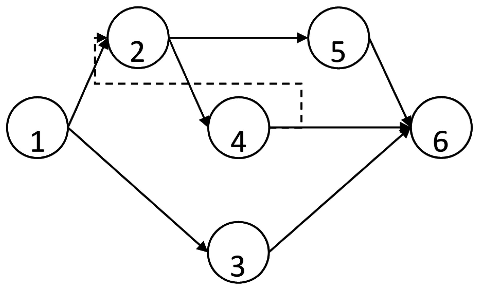
Figure 1. Graphical representation of Ei and δt.
Algorithms 09 00063 g001
Figure 2. Graphical example of MRCPSP/max.
Algorithms 09 00063 g002
Figure 3. Flowchart of the 3-stage procedure.
Algorithms 09 00063 g003
Figure 4. Artificial bee colony flowchart.
Algorithms 09 00063 g004
Figure 5. Graphical representation of swap and insert operators.
Algorithms 09 00063 g005
Table 1. Illustrative data of MRCPSP/max.
Activity (i)Modes ( μ i)Duration (dil;di;diu) R k v Arc Weights (δ)
11--(5,3,1); (4,5,5)
213;3;42(4,1,4); (1,1,7)
22;3;43(2,1,4); (1,6,3)
31;1;24(−1,2,0); (2,3,7)
312;3;51(5)
22;2;23(1)
31;3;55(4)
413;3;43(1,4,9); (3)
22;3;43(7,3,2); (1)
31;2;34(1,2,4); (2)
512;3;34(1)
23;3;45(2)
31;2;27(3)
61---
Table 2. Mode selection rules.
Priority RuleDescription
SFM (Shortest Feasible Mode)Find the feasible mode combination for which the makespan is minimal
LRP (Least Resource Proportion)Choose the mode that leads to the smallest value of the criterion, max( r i μ k ρ K ρ )     μ
LPSRD (Least Product Sum of Resource and Duration)For each activity, choose the execution mode that has the minimum product sum of non-renewable resource usage and its corresponding mode duration, min k = 1 K v ( r i μ k v *   d i μ )     μ
LTRU (Least Total Resource Usage)Choose the execution mode that requires the least total non-renewable usage, min k = 1 K v r i μ k v     μ
LRS (Least sum of Non-renewable Resource)Choose the execution mode that requires the least sum of the ratio of the non-renewable consumption to its corresponding resource limitation, min k = 1 K v r i μ k v R k v     μ
Table 3. Activity priority rules.
Priority RuleReferencesDescription
max ACTIM[51]CPMLSTi
max GCUMRD[52]The sum of the renewable resource demand of the activity considered and the renewable resource demands of all its immediate successors
max MTS[53] | S i ¯ | the total number of successors for activity i
max MIS[53] | S i | the number of immediate successors for activity i
max ROT[54] k = 1 K ρ r i k ρ R k ρ d i sum of the ratio of the renewable resource requirement over the resource availability divided by the activity duration for activity i
max WRUP[55] 0.7 * | S i |   + 0.3 *   k = 1 K ρ r i k ρ R k ρ d i , a weighted sum of the number of immediate successors and an average resource use over all renewable resource types
min EFT[56]EFTi
min LFT[56]LFTi
min SLK[56]LFTi − EFTi
min LNRJ[52] | N S i ¯ | the total number of activities that are not precedence related with activity i
min RSM[57]dij = max[0, (EFTi − LSTj)]
Table 4. Parameters used for the ABC algorithm. MNC, Maximum Number of Cycles.
ParameterValue
Population size30
Abandonment limit5
MNC20
δt (relevant time interval)1
frac0.25
Table 5. Results summary for benchmark instances. Avg. Dev., Average Deviation.
Benchmark SetMM30MM50MM100Overall Average
Optima Found26012384
Stage 1Avg. Dev. vs. BKO0.18%4.57%4.42%3.06%
Stage 2Avg. Dev. vs. BKO9.69%10.13%8.50%9.44%
Avg. Dev. vs. S16.02%5.84%4.27%5.38%
Stage 3Avg. Dev. vs. BKO5.04%5.39%4.37%4.93%
Avg. Dev. vs. S11.10%0.79%−0.12%0.59%
Avg. Dev. vs. S2−5.36%−5.48%−4.62%−5.16%
Table 6. Hypotheses tests for each stage against Best-Known Optima (BKO).
H0: µBKO = µS1
H1: µBKO < µS1
H0: µBKO = µS2
H1: µBKO < µS2
H0: µBKO = µS3
H1: µBKO < µS3
Table 7. p-Values for the hypotheses’ tests.
Benchmark Setp-Value
Stage 1Stage 2Stage 3
MM300.0670.0000.024
MM500.0570.0000.029
MM1000.0490.0000.047
Table 8. Hypotheses tests for each stage against Stage 1.
H0: µS1 = µS2
H1: µS1 < µS2
H0: µS1 = µS3
H1: µS1 < µS3
Table 9. p-Values for hypotheses tests against Stage 1.
Benchmark Setp-Value
Stage 2Stage 3
MM300.0080.318
MM500.0150.379
MM1000.0470.488
Table 10. Hypotheses tests for Stage 2 against Stage 1.
H0: Avg. Dev.S2 − Avg. Dev.S1 = 5%
H1: Avg. Dev.S2 − Avg. Dev.S1 > 5%
Table 11. p-Values for hypotheses tests Stage 2 against Stage 1.
Benchmark Setp-Value
MM301
MM501
MM1001

