1. Introduction
Numerical analysis is a wide-ranging discipline having close connections with mathematics, computer science, engineering and the applied sciences. One of the most basic and earliest problems of numerical analysis are concerned with efficiently and accurately finding the approximate locally unique solution
of an equation of the form
where
F is a Fréchet differentiable operator defined on a convex subset
of
with values in
, where
and
are Banach spaces.
Analytical methods for solving such equations are almost non-existent for obtaining the exact numerical values of the required roots. Therefore, it is only possible to obtain approximate solutions and one has to be satisfied with approximate solutions up to any specified degree of accuracy, by relying on numerical methods which are based on iterative procedures. Therefore, worldwide, researchers resort to an iterative method and a plethora of iterative methods has been proposed [
1,
2,
3,
4,
5,
6,
7,
8,
9,
10,
11,
12,
13,
14,
15]. While using these iterative methods, researchers face the problems of slow convergence, non-convergence, divergence, inefficiency or failure (for detail please see Traub [
14] and Petkovíc et al. [
11]).
The convergence analysis of iterative methods is usually divided into two categories: semi-local and local convergence analysis. The semi-local convergence matter is, based on the information around an initial point, to give criteria ensuring the convergence of iterative procedures. On the other hand, the local convergence is based on the information around a solution, to find estimates of the radii of convergence balls. A very important problem in the study of iterative procedures is the convergence domain. Therefore, it is very important to propose the radius of convergence of the iterative methods.
We study the local convergence analysis of a three step method defined for each
by
where
is an initial point,
,
is any two-point optimal fourth-order scheme and
. The eighth order of convergence of method Equation (
2) was shown in [
13] when
and
for
and
. That is when
is a divided difference of first order of operator
F [
4,
5]. The local convergence was shown using Taylor series expansions and hypotheses reaching up to the fifth order derivative. The hypotheses on the derivatives of
F limit the applicability of method Equation (
2). As a motivational example, define function
F on
,
by
Then for
,we have
and
One can easily see that the function
is unbounded on
at the point
. Hence, the results in [
13] cannot be applied to show the convergence of method Equation (
2) or its special cases requiring hypotheses on the fifth derivative of function
F or higher. Notice that, in particular there is a plethora of iterative methods for approximating solutions of nonlinear equations [
1,
2,
3,
4,
5,
6,
7,
8,
9,
10,
11,
12,
13,
14,
15]. These results show that initial guesses should be close to the required root for the convergence of the corresponding methods. However, how close should an initial guess should be for the convergence of the corresponding method to be possible? These local results give no information on the radius of the ball convergence for the corresponding method. The same technique can be used for other methods.
In the present study, we expand the applicability of method given by Equation (
2) using only hypotheses on the first order derivative of function
F. We also propose the computable radii of convergence and error bounds based on the Lipschitz constants. We further present the range of initial guesses
that tell us how close the initial guesses should be required to guarantee the convergence of the method Equation (
2). This problem was not addressed in [
13]. The advantages of our approach are similar to the ones already mentioned for the method described by Equation (
2).
The rest of the paper is organised as follows: in
Section 2, we present the local convergence analysis of scheme Equation (
2).
Section 3 is devoted to the numerical examples which demonstrate our theoretical results. Finally, the conclusion is given in
Section 4.
2. Local Convergence: One Dimensional Case
In this section, we define some scalar functions and parameters to study the local convergence of method Equation (
2).
Let
,
be given constants. Let us also assume
, be a nondecreasing and continuous function. Define functions
and
p in the interval
by
and parameter
by
Notice that the function is a monotonically increasing function on the interval . We have and for each . Further, define function by .
Then, we have
. By Equation (
3) and the intermediate value theorem, function
has zeros in the interval
. Further, let
be the smallest such zero. Further, define functions
q and
on the interval
by
and
.
Using
and Equation (
3), we deduce that function
has a smallest zero denoted by
.
Finally, define functions
and
on the interval
by
and
Then, we get
and
as
. Denote by
the smallest zero of function
on the interval
. Define
Then, we have that
and for each
and
and stand, respectively for the open and closed balls in with center and radius .
Next, we present the local convergence analysis of scheme Equation (
2) using the preceding notations.
Theorem 1. Let us consider be a Fréchet differentiable operator. Let us also assume be a divided difference of order one. Suppose there exist , a neighborhood of , such that Equation (3) holds and for each andwhere . Moreover, suppose that there exist and such that for each andwhere the radius of convergence r is defined by Equation (4). Then, the sequence generated by method Equation (2) for is well defined, remains in for each and converges to . Moreover, the following estimates holdandwhere the “g” functions are defined by previously. Furthermore, for , the limit point is the only solution of equation in Proof of Theorem 1. We shall show that estimates Equations (
19)–(
21) with the help of mathematical induction. By hypotheses
, Equations (
5) and (
13), we get that
It follows from Equation (
22) and the Banach Lemma on invertible operators [
4,
12] that
is well defined and
Using the first substep of method Equation (
2) for
, Equations (
4), (
6), (
11), (
16) and (
23), we get in turn
which shows Equation (
19) and
. Then, from Equations (
3) and (
12), we see that (
20) follows for
. Hence,
. Next, we shall show that
. Using Equations (
12), (
14) and the strict monotonicity of
q, we obtain in turn that
Hence,
is well defined by the third substep of method Equation (
2) for
. We can write by Equation (
11)
Notice that
, for all
. Hence, we have that
. Then, by Equations (
17) and (
27) we get that
We also have that by replacing
by
in Equation (
28) that
since
.
Then, using the last substep of method Equation (
2) for
, Equations (
4), (
10), (
13)–(
15), (
19), (
20) (for
), (
23), (
26) and (
29), we obtain that
which shows Equation (
21) for
and
. By simply replacing
,
by
,
in the preceding estimates we arrive at Equations (
19)–(
21) for all
. Using the monotonicity of
on the interval
and (
21), we have with
where
. This yields
and
.
Finally, to show the uniqueness part, let
be such that
. Set
. Then, using Equation (
13), we get that
Hence,
. Then, in view of the identity
, we conclude that
. It is worth noticing that in view of Equations (
12), (
21), (
31) and the definition of functions
the convergence order of method Equation (
2) is at least
λ. ☐
Remark 1 - (a)
In view of Equation (
13) and the estimate
condition Equation (
17) can be dropped and
M can be replaced by
or
since
- (b)
The results obtained here can be used for operators
F satisfying the autonomous differential equation [
4,
5] of the form
where
P is a known continuous operator. Since
we can apply the results without actually knowing the solution
As an example, let
Then, we can choose
.
- (c)
The radius
was shown in [
4,
5] to be the convergence radius for Newton’s method under conditions (
11) and (
12). It follows from Equation (
4) and the definition of
that the convergence radius
r of the method Equation (
2) cannot be larger than the convergence radius
of the second order Newton’s method. As already noted in [
4,
5]
is at least the convergence radius given by Rheinboldt [
12]
In particular, for
we have that
and
That is our convergence radius
r is at most three times larger than Rheinboldt’s. The same value for
given by Traub [
14].
- (d)
We shall show how to define function
and
l appearing in condition Equation (
3) for the method
Clearly method Equation (
33) is a special case of method Equation (
2). If
then method Equation (
33) reduces to Kung-Traub method [
14]. We shall follow the proof of Theorem 1 but first we need to show that
. By assuming the hypotheses of Theorem 1, we get that
The function
, where
, has a smallest zero denoted by
in the interval
. Set
. Then, we have from the last substep of method Equation (
33) that
It follows from Equation (
34) that
and
Then, the convergence radius is given by
3. Numerical Example and Applications
In this section, we will verify the validity and effectiveness of our theoretical results which we have proposed in
Section 2 based on the scheme proposed by Sharma et al. [
13]. For this purpose, we shall choose a variety of nonlinear equations and systems of nonlinear equations which are mentioned in the following examples including motivational example. At this point, we will chose the following methods
and
denoted by
,
and
, respectively.
First of all, we require the initial guesses
which gives the guarantee for convergence of the iterative methods. Therefore, we shall calculate the values of
,
,
,
,
,
and
r to find the range of convergence domain, which are displayed in the
Table 1,
Table 2,
Table 3 and
Table 4 up to 5 significant digits. However, we have the values of these constants up to several number of significant digits. Then, we will also verify the theoretical order of convergence of these methods for scalar equations on the basis of the results obtained from computational order of convergence and
. In the
Table 5 and
Table 6, we display the number of iteration indexes
, approximated zeros
, residual errors of the corresponding function
, errors
(where
),
and the asymptotic errors constant
. In addition, We will use the formulas proposed by Sánchez et al. in [
7] to calculate the computational order of convergence (COC), which is given by
or the approximate computational order of convergence (ACOC) [
7]
We calculate the computational order of convergence, asymptotic errors constant and other constants up to several numbers of significant digits (minimum 1000 significant digits) to minimise the round off errors.
In the context of systems of nonlinear equations, we also consider a nonlinear systems in Example 3 to check the proposed theoretical results for nonlinear systems. In this regard, we displayed the number of iteration indexes
, residual errors of the corresponding function
, errors
(where
),
and the asymptotic errors constant
in the
Table 7 and
Table 8.
As we mentioned in the earlier paragraph, we calculate the values of all the constants and functional residuals up to several numbers of significant digits but, due to the limited paper space, we display the values of up to 15 significant digits. Further, the values of other constants, namely, up to 5 significant digits and the values and are up to 10 significant digits. Furthermore, the residual errors in the function/systems of nonlinear functions () and the errors are displayed up to 2 significant digits with exponent power which are mentioned in the following tables corresponding to the test function. However, a minimum of 1000 significant digits are available with us for every value.
Furthermore, we consider the approximated zero of test functions when the exact zero is not available, which is corrected up to 1000 significant digits to calculate . During the current numerical experiments with programming language Mathematica (Version 9), all computations have been done with multiple precision arithmetic, which minimises round-off errors.
Further, we use
and function
defined by Equation (
35) in all the examples.
Example 1. Let . Define F on for by Then the Fréchet-derivative is given by Then, for we get , and . We calculate the radius of convergence, the residual errors of the corresponding function (by considering initial approximation in the methods ), errors (where ), and the asymptotic errors constant , which are displayed in the Table 1 and Table 5. Example 2. Let and define function F on by Then, for we obtain that and . Hence, we obtain all the values of constants and residual errors in the functions, etc., which we have described earlier in the Table 2 and Table 6. Example 3. Let . Define F on for by Then the Fréchet-derivative is given by Notice that , and . Hence, we calculate the radius of convergence, the residual errors of the corresponding function (by considering initial approximation in the methods ), errors (where ) and other constants, which are given in the Table 3 and Table 7. Example 4. Returning back to the motivational example in the introduction of this paper, we have , an . We display all the values of constants and residual errors in the functions which we have described earlier in the Table 4 and Table 8. 3.1. Results and Discussion
Sharma and Arora’s study was only valid for simple roots of the scalar equation. The order of convergence was shown using Taylor series expansions, and hypotheses up to the fourth order derivative (or even higher) of the function involved, which restricts the applicability of the proposed scheme. However, only the first order derivatives appear in the proposed scheme. In order to overcome this problem, we propose the hypotheses only up to the first order derivative. the applicability of the proposed scheme can be seen in the Examples 1, 3 and motivational example, where earlier studies were not successful. We also provide the radius of convergence for the considered test problem which gives the guarantee for the convergence.
In addition, we have also calculated residual error in the each corresponding test function and the difference between the exact zero and approximated zero. It is straightforward to say from the
Table 5,
Table 6,
Table 7 and
Table 8 that the mentioned methods have smaller residual error in each corresponding test function and a smaller difference error between the exact and approximated zero. So, we can say that these methods converge faster towards the exact root. Moreover, the mentioned methods also have simple asymptotic error constant in most of the test functions which can be seen in the
Table 5,
Table 6,
Table 7 and
Table 8. The dynamic study of iterative methods via basins of attraction also confirm the faster convergence. However, one can find different behaviour of our methods when he/she considers some different nonlinear equations. The behaviour of the iterative methods mainly depends on the body structure of the iterative method, considered test function, initial guess and programming software, etc.
4. Basin of Attractions
In this section, we further investigate some dynamical properties of the attained simple root finders in the complex plane by analysing the structure of their basins of attraction. It is known that the corresponding fractal of an iterative root-finding method is a boundary set in the complex plane, which is characterised by the iterative method applied to a fixed polynomial
, see, e.g., [
6,
16,
17]. The aim herein is to use the basin of attraction as another way for comparing the iterative methods.
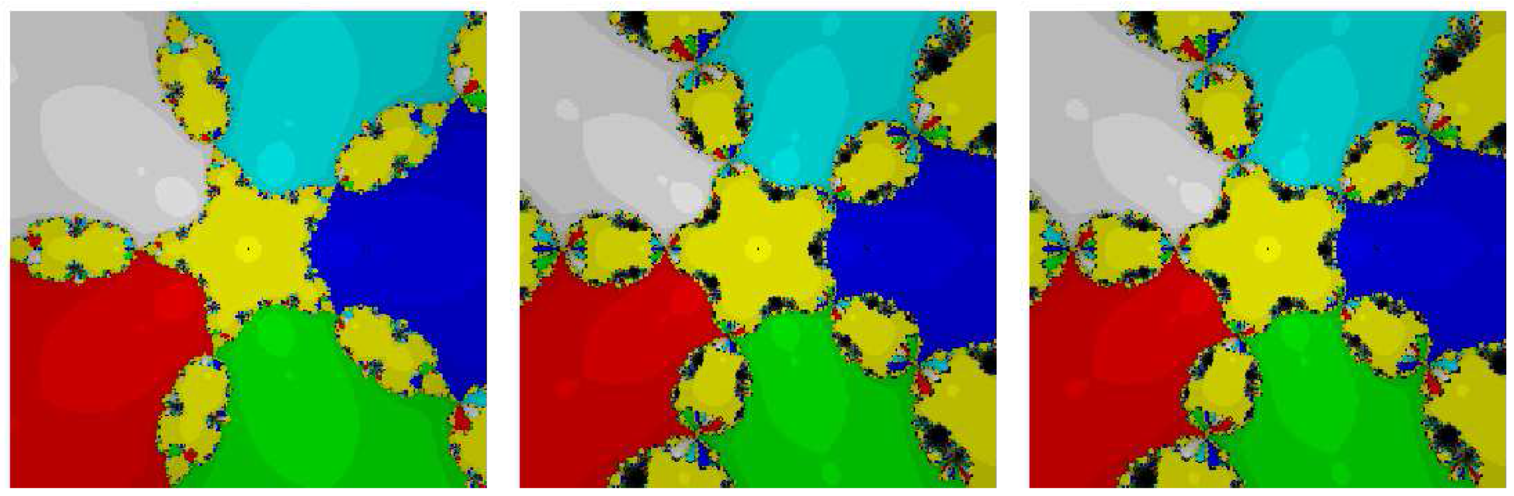
From the dynamical point of view, we consider a rectangle with a grid, and we assign a color to each point according to the simple root at which the corresponding iterative method starting from converges, and we mark the point as black if the method does not converge. In this section, we consider the stopping criterion for convergence to be less than wherein the maximum number of full cycles for each method is considered to be 100. In this way, we distinguish the attraction basins by their colours for different iterative methods.
Test Problem 1. Let
having simple zeros
. It is straightforward to see from
Figure 1 that the method
is the best method in terms of less chaotic behaviour to obtain the solutions. Further,
also has the largest basins for the solution and is faster in comparison to all the mentioned methods namely,
and
.
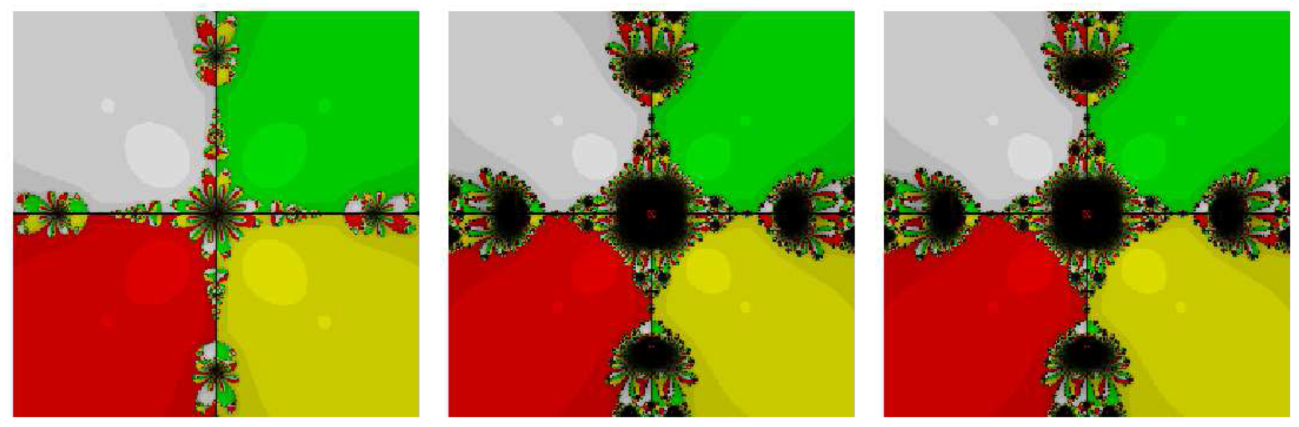
Test Problem 2. Let
having simple zeros
. Based on
Figure 2, it is observed that all the methods, namely,
,
and
have almost zero non convergent points. However, method
has a larger and brighter basin of attraction as compared to the methods
and
. Further, the dynamics behavior of the method
on the boundary points is less chaotic than other methods
and
.
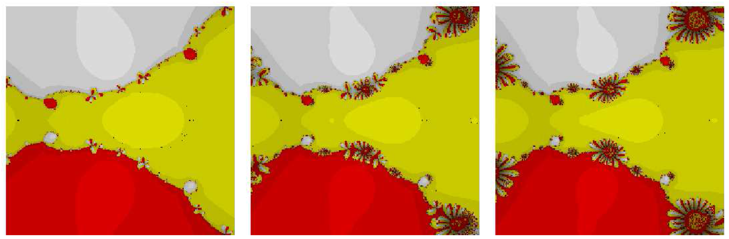
Test Problem 3. Let having simple zeros
. It is concluded on the basis of
Figure 3, that the method
has a much lower number of non convergent points as compared to
and
(in fact we can say that method
has almost zero non convergent points in this region). Further, the dynamics behaviors of the methods
and
are shown to be very chaotic on the boundary points.
5. Conclusions
Commonly, researchers have mentioned that the initial guess should be close to the required root for the granted convergence of their proposed schemes for solving nonlinear equations. However, how close should the initial guess be if it is required to guarantee the convergence of the proposed method? We propose the computable radius of convergence and errors bound by using Lipschitz conditions in this paper. Further, we also reduce the hypotheses from fourth order derivative of the involved function to only first order derivative. It is worth noting that the method in Equation (
2) does not change if we use the conditions of Theorem 1 instead of the stronger conditions proposed by Sharma and Arora (2015). Moreover, to obtain the errors bound in practice and order of convergence, we can use the computational order of convergence which is defined in numerical
Section 3. Therefore, we obtain in practice the order of convergence in a way that avoids the bounds involving estimates higher than the first Fréchet derivative.
In an earlier study, Sharma and Arora mentioned that their work is valid only for
. However, in our study we have shown that this scheme will work in any space. The order of convergence for the proposed scheme may be unaltered or reduce in another space because it depends upon the space and function (for details please see the numerical section). Finally, on account of the results obtained in
Section 3, it can be concluded that the proposed study not only expands the applicability but also gives the computable radius of convergence and errors bound by the scheme given by Sharma and Arora (2015), for obtaining simple roots of nonlinear equations as well as systems of nonlinear equations.


