Article

Comparison of Different Algorithms to Orthorectify WorldView-2 Satellite Imagery

Department of Sciences and Technologies, University of Naples “Parthenope”, Centro Direzionale Isola C4, Naples 80143, Italy
*
Author to whom correspondence should be addressed.
Algorithms 2016, 9(4), 67; https://doi.org/10.3390/a9040067
Submission received: 27 June 2016 / Revised: 27 September 2016 / Accepted: 30 September 2016 / Published: 11 October 2016

Abstract

:
Due to their level of spatial detail (pixel dimensions equal to or less than 1 m), very high-resolution satellite images (VHRSIs) need particular georeferencing and geometric corrections which require careful orthorectification. Although there are several dedicated algorithms, mainly commercial and free software for geographic information system (GIS) and remote sensing applications, the quality of the results may be inadequate in terms of the representation scale for which these images are intended. This paper compares the most common orthorectification algorithms in order to define the best approach for VHRSIs. Both empirical models (such as 2D polynomial functions, PFs; or 3D rational polynomial functions, RPFs) and rigorous physical and deterministic models (such as Toutin) are considered. Ground control points (GCPs) and check points (CPs)—whose positions in the image as, well as in the real world, are known—support algorithm applications. Tests were executed on a WorldView-2 (WV-2) panchromatic image of an area near the Gulf of Naples in Campania (Italy) to establish the best-performing algorithm. Combining 3D RPFs with 2D PFs produced the best results.

1. Introduction

Very high-resolution satellite images (VHRSIs) are widely used in several application fields, at both scientific and commercial levels, because of their detailed information (pixel dimensions equal to or less than 1 m in panchromatic band).
The geometric use of these images requires careful orientation and orthorectification in order to georeference the images and correct the geometric deformations introduced during acquisition [1].
Remotely sensed images contain such significant geometric distortions that they cannot be used directly with map-based products in a geographic information system (GIS) [2]. This characteristic is particularly pertinent to VHRSIs for several reasons (e.g., the reduced dimensions of the pixels and the off-nadir viewing).
Well-corrected and georeferenced VHRSIs such as IKONOS, WorldView-2 (WV-2), Quickbird, GeoEye, and Komposat are used for many purposes, i.e., map creation and updating, emergency mapping [3,4,5,6], vegetation mapping [7], coastline identification [8,9], etc. Production of high-resolution colored orthophotos can be achieved [10] by introducing pan-sharpening algorithms [11,12]. In the case of WV-2, the presence of eight multispectral bands instead of the traditional four provide a more powerful source of information, thus increasing thematic accuracy. Jawak et al. [13] demonstrate how WV-2 imagery, compared to previous sensors, improves the identification of land-cover targets, and consequently improves the land-cover classification.
To correct imagery geometric distortions, models and mathematical functions are necessary: either 2D/3D empirical models (such as 2D/3D polynomial or 3D rational polynomial functions, RPFs) or rigorous 2D/3D physical and deterministic models [2]. A physical model should model the platform (attitude, velocity, and altitude), sensor (field of view, panoramic effect), world (ellipsoid and 3D relief), and cartographic projection distortions [14].
Such 2D/3D empirical models can be used when the parameters of the acquisition systems or a rigorous 3D physical model are not available. In addition, they are based on different mathematical functions (2D or 3D polynomial functions, 3D rational functions) [15].
Physical models (also called rigorous models) are based on a standard photogrammetric approach, where the collinearity equations link the image and the ground coordinates, and the parameters involved have a physical meaning. In addition, knowledge regarding the sensor on the specific satellite and orbit characteristics is required [16].
These 2D/3D empirical models do not reflect the real physical condition of imaging, but they define it approximately. Three different sensor replacement models are defined in ISO 19130 “Geographic Information—Imagery Sensor Models for Geopositioning”: (1) simple polynomial fitting; (2) rational function model—RFM; and (3) universal sensor model—USM [14]. Simple polynomial fitting is useful only for low- and medium-resolution satellite images [17] and can be adopted for VHRSIs in small area mapping. In fact, we can also assume that the sensor moves linearly in space and that the attitude is almost unchanged [18]. The relationship between the position of a point on the image and the corresponding point on the object is represented by polynomial functions. The coefficients of each polynomial are computed using an appropriate number of ground control points (GCPs) with known locations (X, Y) on the map and easy detections (X’, Y’) in the image [19].
An RFM matches the image and object spaces through a ratio of two polynomial functions to compute the image row, and a similar ratio to compute the image column [20]. Also, in this case an appropriate number of GCPs is necessary to calculate the coefficients of each polynomial, named RPCs (rational polynomial coefficients). RPCs are widely adopted by image vendors and government agencies, who do not want to provide any satellite/sensor information with the image, and by commercial workstation suppliers; consequently, the various image vendors around the world provide third-order RF parameters [21]. RFMs have been used to approximate physical sensor models for many years due to their capability to maintain the full accuracy of different physical sensor models, their unique characteristic of sensor independence, and real-time calculation [22].
With USMs, an image scene is divided into multiple subdivisions or sections and RFM is applied to each section; the modified polynomials are of a variable order (up to the fifth power of the two horizontal coordinates and up to the third power for elevation); the denominator polynomials are usually omitted; image positional correction tables can be incorporated; and the ground coordinates can be expressed in any ground coordinate system [23].
Several applications about the use of 2D/3D empirical models as well as 2D/3D physical and deterministic models to orthorectify VHRSIs are available in literature. Chmiel et al. [24] compared rigorous approach and RFM to achieve the best geometric accuracy in orthorectified imagery products obtained from IKONOS (Geo Ortho-kit), QuickBird (Standard OrthoReady), and EROS 1A level data. Wolniewicz [25] analyzed the influence of the number and distribution of GCPs on the planimetric accuracy reached in the final QuickBird- and IKONOS-corrected panchromatic image using different orthorectification methods. Afify and Zhang [26] assessed the attainable geometric accuracies of RFMs applied to IKONOS and Quickbird images when user adjustments are introduced. Aguilar et al. [27] compared results recorded for IKONOS (Geo Ortho-kit) and QuickBird basic imagery, applying two different sensor models: (1) a 3D rational function refined by the user with zero- or first-order polynomial adjustment and (2) the 3D Toutin physical model. The influence of the number of GCPs on the geometric accuracy reached with RFM applied to GeoEye-1 images was analyzed by Maglione et al. [28].
This paper describes orthorectification that was conducted on WorldView-2 (WV-2) imagery using several algorithms which are available in common commercial and free software. Both rigorous and empirical approaches are considered and positional accuracies of the results are compared and discussed in order to define the best algorithm or the best combination. To our knowledge this, is the first work that compares several methods (including polynomial functions and rational functions, with variable number of GCPs) on WV-2 imagery. The paper is organized as follows. Section 2 describes the data and methods; various algorithms are applied to WV-2 imagery regarding the area around Vesuvius. Section 3 presents and discusses the results. Finally, Section 4 draws some conclusions.

2. Materials and Methods

2.1. WorldView2 Imagery

Launched in October 2009 by DigitalGlobe, the WV-2 satellite is positioned at an altitude of 770 km, with an orbit inclination of 97.2° and a period of 100 min. The revisited frequency is 1.1 days at nadir and 3.7 days at 20° off-nadir. The swath width, at nadir, is 16.4 km [29]. This satellite is part of DigitalGlobe’s constellation, which now also includes WorldView-3 [30,31,32]. The WV-2 satellite has two push-broom scanners which acquire panchromatic and multispectral images, respectively. The panchromatic images have a spatial resolution of 0.46 m, resampled to 0.50 m for commercial purposes, and the spectral interval is 0.450–0.800 μm. The multispectral images have a spatial resolution of 1.85 m, resampled to 2 m for commercial purposes; they are acquired in eight bands: Coastal (0.400–0.450 μm); Blue (0.450–0.510 μm); Green (0.510–0.580 μm); Yellow (0.585–0.625 μm); Red (0.630–0.690 μm); Red Edge (0.705–0.745 μm); Near-IR1 (0.770–0.895 μm); Near-IR2 (0.860–1.040 μm). The radiometric resolution for both panchromatic and multispectral images is 11 bits [29].

2.2. The Area Considered

In this study, WV-2 imagery concerning the area around Vesuvius (Campania, Italy) was considered (Figure 1). The dataset was acquired on 22 April 2015 and supplied by the provider as Ortho Ready Standard product (ORS2A), which means it had already been rectified using the average terrain elevation of the scene (low accuracy) [33]. The scene is georeferenced in the UTM/WGS84 33 N zone T coordinates system and extends from 40°46′22.06′′ north to 40°51′46.53′′ north in latitude and 14°20′2.74′′ east to 14°24′40.70′′ east in longitude.
This area is particularly interesting due to both its anthropological and natural features. In fact, most of the area is within the Vesuvius National Park, founded in 5 June 1995, which houses 610 vegetable species and 229 vertebrates and invertebrates [34]. The area also has one of the highest urban densities in Europe and includes the archeological remains of Pompeii, the ancient town that was destroyed by the eruption of Vesuvius in 79 AD. Thus, a high-performance VHRSI such as WV-2 would clearly support research activities in many fields, if corrected and georeferenced.

2.3. Algorithms for Orthorectification

In this section, several algorithms that are present in the software most commonly used for image orthorectification are described.
According to Toutin [2], whatever the mathematical functions used, the geometric correction method and processing steps are: acquisition of image; acquisition of the GCPs and check points (CPs) with image coordinates and map coordinates X, Y, Z; computation of the unknown parameters of the mathematical functions used for the geometric correction model; and image rectification with or without digital elevation model (DEM).
The two-dimensional (2D) polynomial model has been adopted for image rectification since the 1970s [35]. It relates images coordinates (X’, Y’) to cartographic coordinates (X, Y) by the following equations:
x = i = 0 m 1 j = 0 m 2 a i j x i y j ,   y = i = 0 m 1 j = 0 m 2 b i j x i y j
If n is the order of the equation, the following relations are valid:
0 m 1 n ; 0 m 2 n ; m 1 + m 2 n .
The 2D polynomial function model of the first order (6 parameters) corrects the image by a rotation, a translation in x and y, scaling along both axes and an obliquitous transformation. The 2D first-order polynomial function is also called affine transformation. The 2D polynomial function model of second order (12 parameters) adds to the previous transformation’s correction of the torsion and convexity along both axes. A cubic polynomial function (20 parameters) further increases the correction flexibility, in a way that does not necessarily correspond to any physical reality of the image acquisition system [36].
By substituting the coordinate values of GCPs in Equation (1), polynomial coefficients (alij and blij) can be calculated. Consequently, the new location of each pixel in the cartographic plane can be defined. The minimum number of GCPs needed is established by the order n of the polynomial functions according to the formula [37]:
N min G C P s = ( n + 1 ) ( n + 2 ) 2
To increase the positional accuracy of the resulting image, a greater number of GCPs is chosen, which are distributed regularly. Thus differences between map coordinates and corrected image coordinates for the same features tend to be reduced. To evaluate the quality of the results, errors not only for GCPs but also for other points, named check points (CPs), are considered [2,38].
Using polynomial functions is a very uncomplicated method to orthorectify VHRSI: often considered outdated, they correct for basic planimetric distortion at the GCPs; because they do not take ground elevation into consideration, they are limited to small and flat areas [39].
3D rational polynomial functions (RPFs) may be more useful. They define a relationship between the image coordinates (x’, y’) and the 3D object coordinates (X, Y, Z) [23,40].
Specifically:
x = P 1 n ( X,Y,Z ) P 2 n ( X,Y,Z )    y = P 3 n ( X,Y,Z ) P 4 n ( X,Y,Z )
where P 1 n , P 2 n , P 3 n , P 4 n are usually cubic polynomials. Each of these includes 20 coefficients and can be expressed as:
P l n ( X , Y , Z ) = i = 0 m 1 j = 0 m 2 k = 0 m 3 a l i j k X i Y j Z k
where:
n = 3 l = 1 , 2 , 3 , 4 0 m 1 3 ; 0 m 2 3 ; 0 m 3 3 ; m 1 + m 2 + m 3 3
Equations in (4) are known in the literature as Upward RFM, as they enable the image coordinates to be obtained starting from the 3D coordinates of a ground point [41].
Substituting P in (4) with the polynomials in (5) and eliminating the first coefficient in the denominator, there are 39 RPF coefficients in each equation: 20 coefficients in the numerator and 19 (and the constant 1) in the denominator [42]. In order to solve the 78 coefficients, at least 39 GCPs are required [43].
The 78 coefficients are calculated by the data provider considering the position of the satellite at the time of image acquisition. They are then included in the RPC (rational polynomial coefficient) file.
However, they can also be calculated using GCPs [43], as in the case above for polynomial functions (PFs). At least 39 of them are needed. In fact, if the camera model is not available, the ground control points need to be selected in a conventional way; that is, through collimation of the homologous points on the cartography or DEM (digital elevation model) or through specific GPS (Global Positioning System) survey campaigns [44]. Usually the Equations in (4) are resolved using a least squares iterative process, on the basis of the measurement of a large number of GCPs.
The accuracy of the results depends on the number and the distribution of GCPs. Several GCPs (more than 39) with a regular planimetric and altimetric distribution contribute to the high quality of the results [17,45,46]. A DEM of the whole area is also required for RPFs.
By applying PFs as well as RPFs to the primary image, a matrix of “empty” cells is computed. To calculate the radiometric value to be assigned to each pixel, a resampling method, such as nearest neighbor, bilinear interpolation, or cubic convolution, is used [47,48]. The nearest-neighbor algorithm is used for this application because it preserves the original radiometric values, which is fundamental for further image processes (calculation of vegetation indexes, classifications, etc.).
Several algorithms are described in the literature for VHRSI orthorectification using rigorous physical models. Based on the collinearity equations, they reconstruct the geometry of the scene during the image acquisition through the knowledge of parameters concerning both the platform and the sensor.
The traditional photogrammetric method of transforming from object space to image space using collinearity equations is highly suited to frame cameras, but not to pushbroom sensor products [23]. In fact, unlike the traditional frame-based aerial photos, each line of the linear array image is collected in a pushbroom fashion at a different instant of time; therefore, the perspective geometry is only valid for each line whereas it is close to a parallel projection in along-track direction; in addition, for each line, there is a different set of (time-dependent) values for the exterior orientation elements [49]. For 1-meter GSD pushbroom sensors such as IKONOS, fully parametrized camera models are extremely complex and difficult to implement; this is highlighted in the IKONOS System Geometric and Mathematical Model document that consists of 183 pages [50].
OrthoEngine—PCI geomatics software (PCI, 2016) supplies Toutin’s rigorous model [51,52]. Originally developed for SPOT, the model was also later extended for Landsat and satellites with synchronous imaging acquisition i.e., IKONOS II, QuickBird [53], WV-2, Komposat-2, and OrbView [54].
Other examples of rigorous models are mentioned in the literature, i.e., the model implemented in SISAR, which is a software for high-resolution satellite images at the Area di Geodesia e Geomatica—Sapienza Università di Roma. The approximate values of the physical parameters can be computed thanks to the information contained in the metadata file provided with each image and corrected by a least squares estimation process based on an appropriate number of GCPs [55].
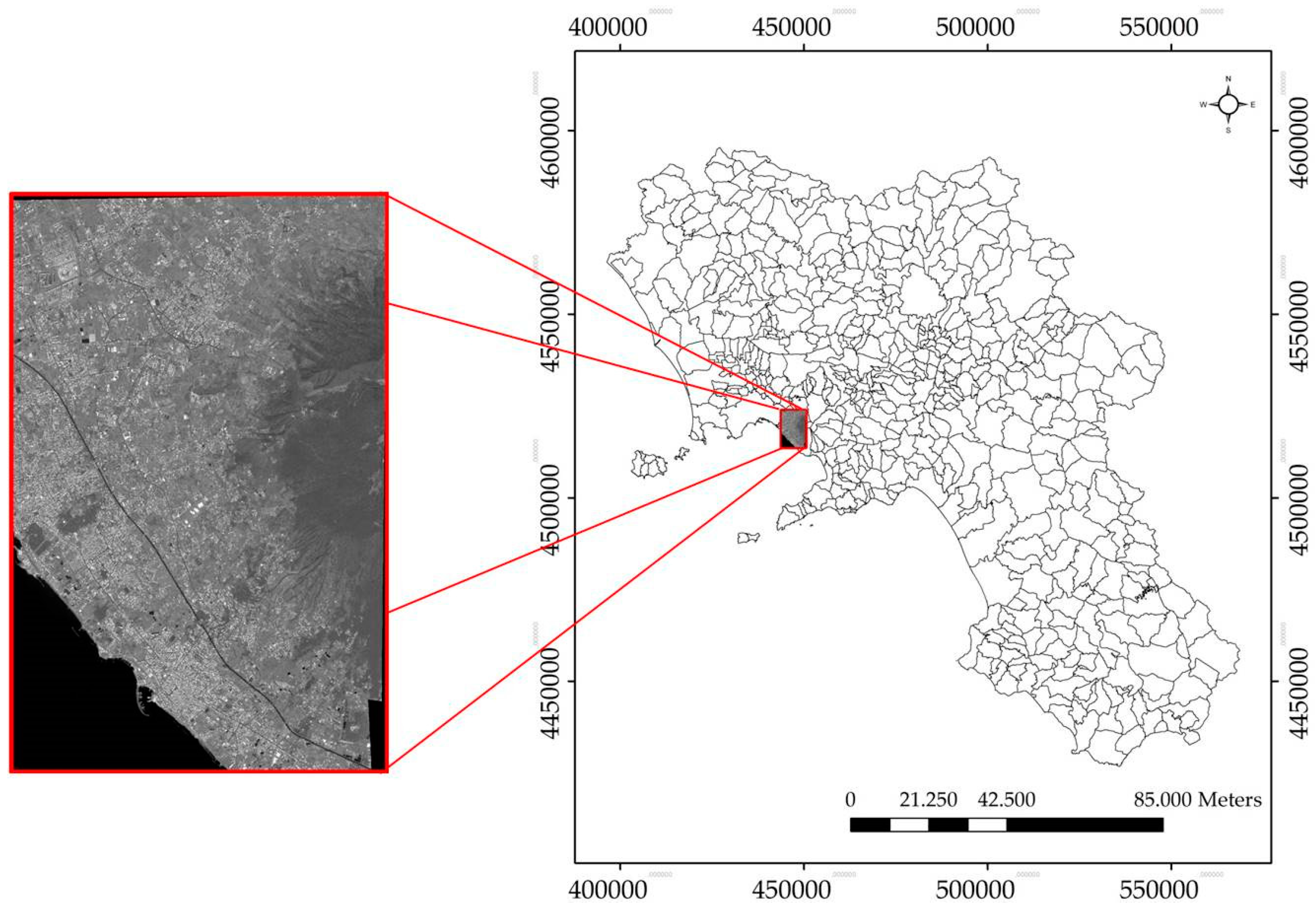
In this work orthorectification processes were carried out on the WV-2 panchromatic image using PCI Geomatica OrthoEngine Version 2015. The following algorithms were applied:
  • 2D PFs;
  • 3D RPFs with original RPCs;
  • 3D RPFs without original RPCs;
  • Toutin’s rigorous model;
  • A combination of 3D RPFs and 2D PFs.
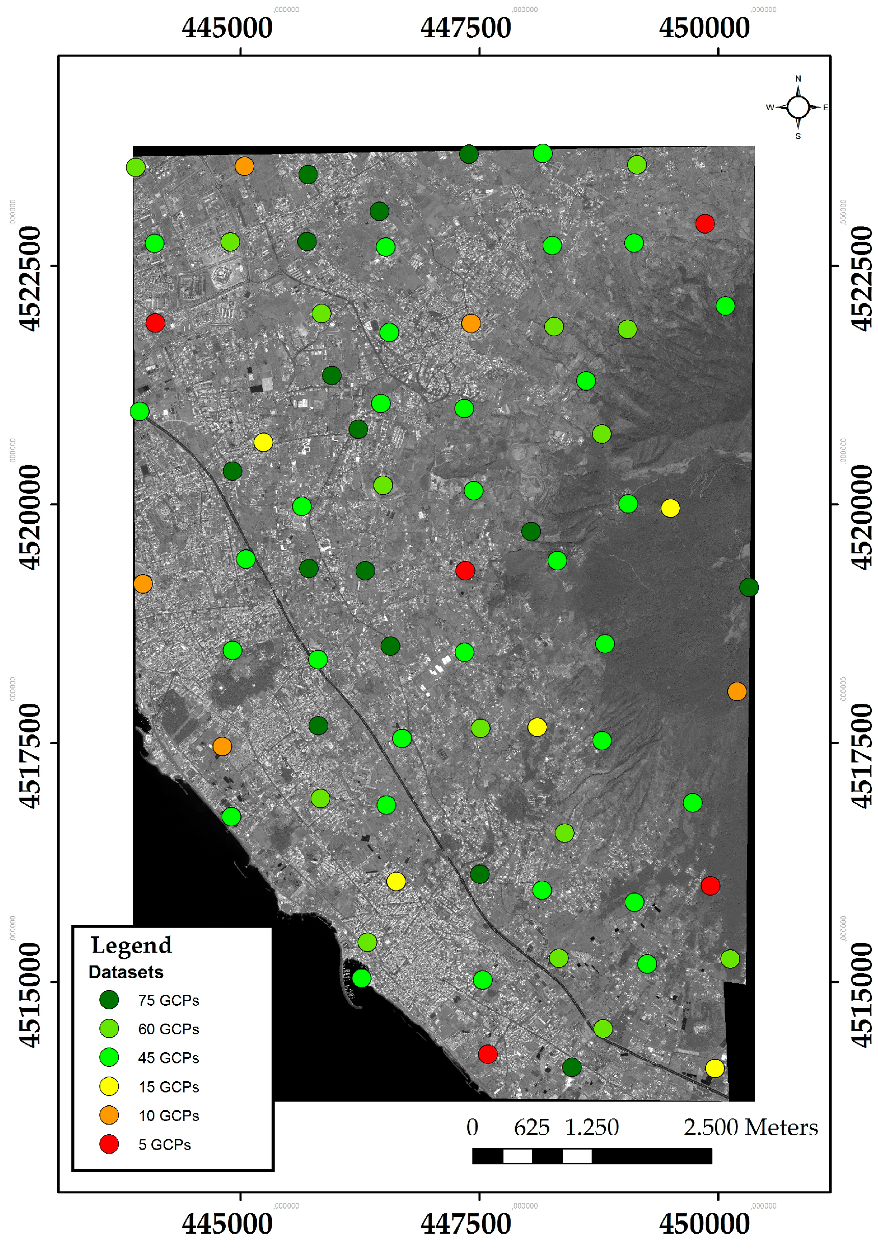
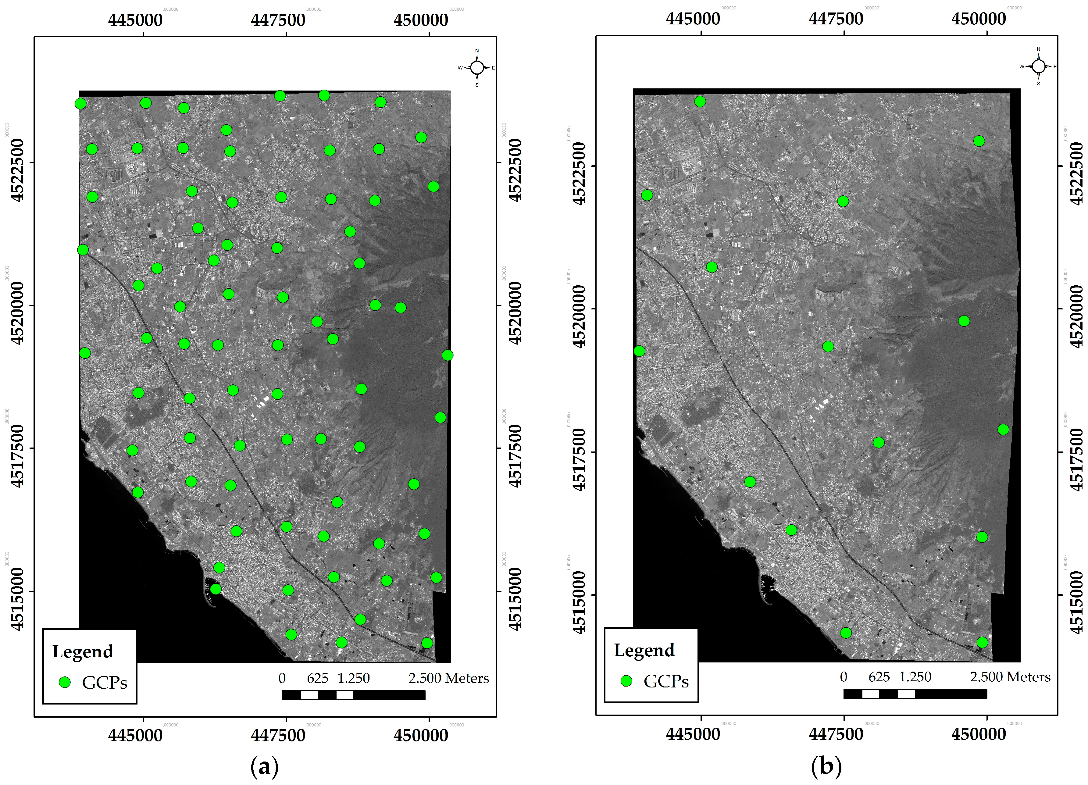
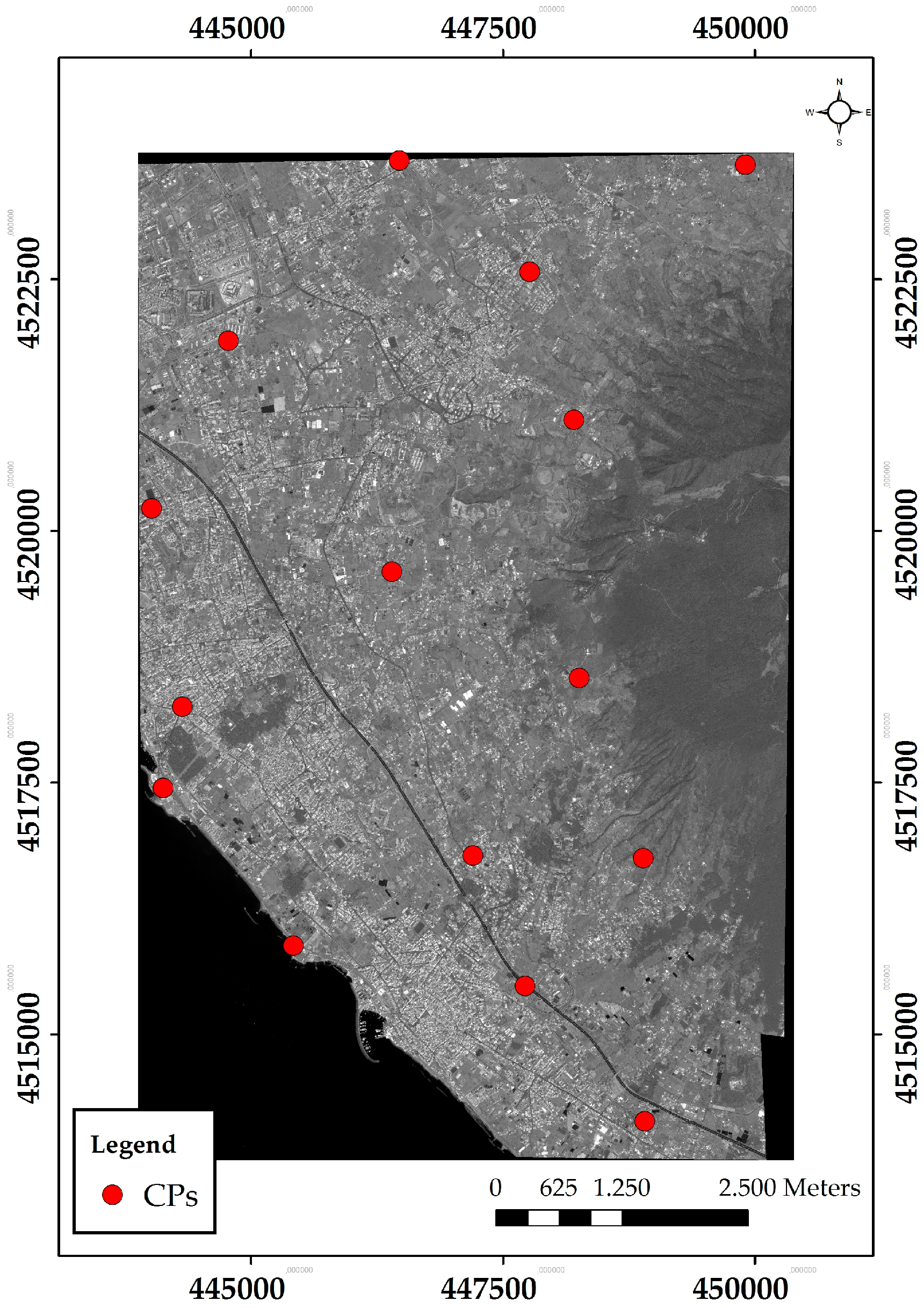
Both GCPs and CPs were homogeneously distributed over the study area and located on well-defined features. Clearly, the source, accuracy, distribution and number of GCPs and CPs are very important for a correct orthorectification [
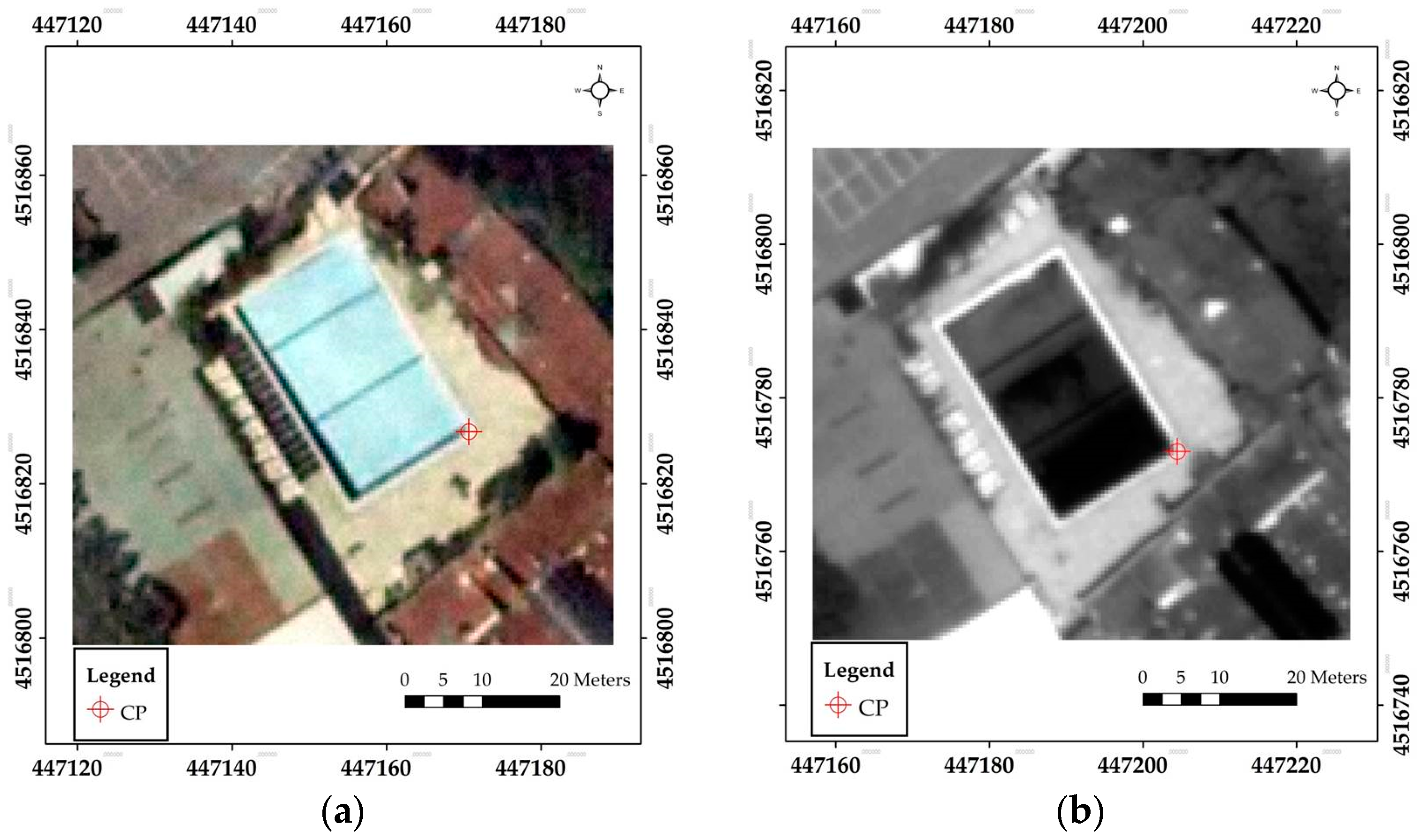
2]. To obtain a reliable measurement of GCPs and CPs with adequate planimetric accuracy, their (x, y) coordinates in UTM-WGS84 were derived from orthophotos of Campania with 0.20 m resolution (nominal scale: 1:5000). It should be noted that errors may occur when manually selecting corresponding points. Thus, specific GCPs and CPs were detected in well-defined locations such as road junctions and corners of buildings or swimming pools. For any ambiguous points, Canny edge detection algorithm [56] was used to support the identification of the corresponding points. In accordance with the literature [25], this helps in ensuring that the accuracy of the GCP and CP identification on the imagery was definitely below one pixel. Figure 2 reports an example of CP identification.
GCP and CP elevations were obtained by DEMs of the study area with a different horizontal resolution (cell size: 1 m, 20 m, 75 m). The DEM with a cell size of 1 m derived from laser-scanning data was supplied by the local administration (Provincia di Napoli) which indicates residuals of 0.16 m between the heights from the grid and those of the 3D points acquired with the RTK (real-time kinematic) survey. The DEM with a cell size of 20 m was provided by IGM (Istituto Geografico Militare), which indicates residuals of 7–10 m between the heights from the grid and those of the 3D points in plane and hilly zones. The DEM with a cell size of 75 m was provided by ISPRA (Istituto Superiore per la Protezione e la Ricerca Ambientale) and presents a vertical accuracy of 16–22 m in the considered area.
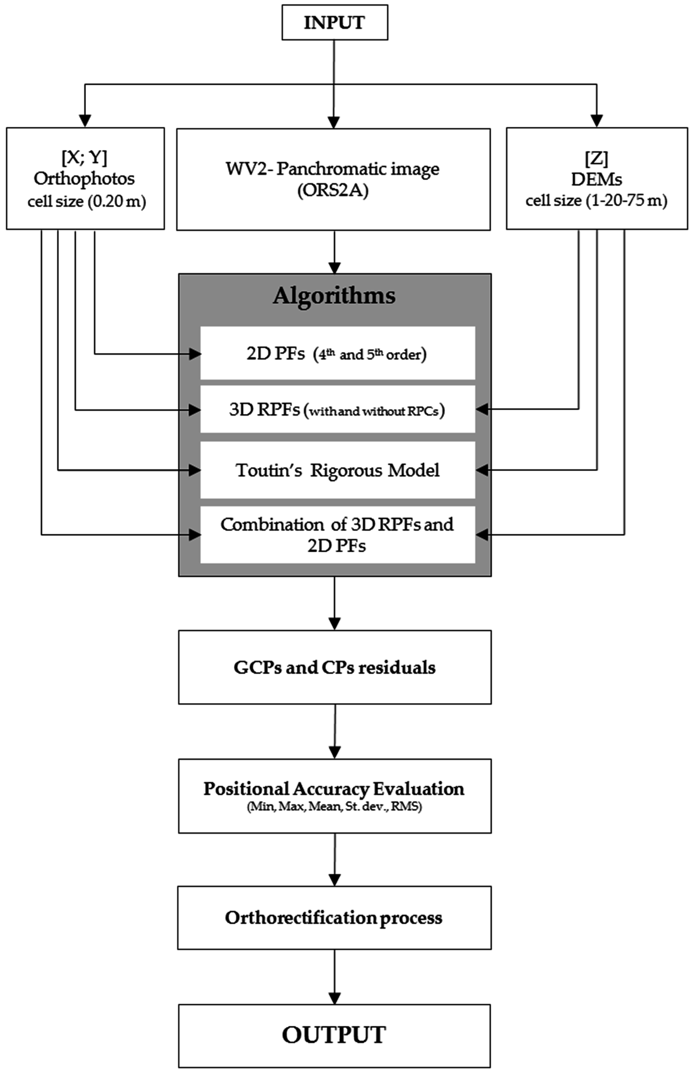
The flowchart in Figure 3 shows the inputs (orthophotos, WV-2 panchromatic image, DEMs), the algorithms used (2D PFs—fourth- and fifth-order; 3D RPFs with and without RPCs; Toutin’s rigorous model; and a combination of 3D RPFs and 2D PFs), and the most important steps (GCP and CP residuals calculation, positional accuracy evaluation based on minimum, maximum, mean, standard deviation, RMS calculation, orthorectification process, and output).
The orthorectification in two steps was introduced to increase the geopositional accuracy of the final WV-2 panchromatic image. In the first step, the best resulting 3D RPFs model (75 GCPs–15 CPs, DEM = 1 m) was applied. For the second step, first-order PFs using 15 GCPs was performed on the orthoimage resulting from the first step.

3. Results and Discussion

The positional accuracy of the primary panchromatic image was tested using 15 CPs. Figure 4 reports the CP distribution in the WV-2 primary panchromatic image. Table 1 shows the statistical values (minimum, maximum, mean, standard deviation, RMS) of errors in these CPs. The low level of positional accuracy of the primary image (RMS = 84.589 m) is evident compared with the pixel dimensions.
The performance of each rectification was evaluated by the residuals obtained for GCPs and CPs in XY direction. Figure 5 illustrates the distribution of all GCPs datasets (5-10-15-45-60-75) in WV-2 primary panchromatic image. A homogenous distribution was attempted for each group of GCPs.
For all the tests performed, 15 CPs (the same as the previous test on the primary image) were introduced. Statistical values of these errors are reported in the following tables.
Table 2 shows how for both fourth- and fifth-order PFs, 60 GCPs produce better results than 45 GCPs while the introduction of another 15 GCPs leads to small increases in accuracy. However, the results are not suitable (RMS for CPs = 10–25 m) in terms of the image geometric resolution (0.5 m).
Table 3 and Table 4 show how the original RPC file supplied by image provider limits CP residuals using a low number of GCPs (i.e., when a DEM with a cell size of 1 m is used, only 5 GCPs mean that the RMS on CPs can be limited to 3.272 m). Although height accuracy is less important than planimetric accuracy, the influence of DEM resolution on elevation extraction is also evident (e.g., with 15 GCPs, the RMS residuals for CPs was 3.747 m using DEM with a 75 m cell size and 1.688 m using DEM with a 1 m cell size.
Table 5 shows that to achieve good results a great number of GCPs as well as a high-resolution DEM are required to calculate RPCs.
Table 6 and Table 7 show how Toutin’s rigorous model obtains a good performance using a low number of GCPs and a high-resolution DEM (e.g., with 15 GCPs, RMS residuals for CPs was 4.129 m using DEM with a 75 m cell size and 1.737 m using DEM with a 1 m cell size).
Table 8 reports the results obtained using the combination of RPF and PF algorithms. The GCPs used in this case are illustrated in Figure 6. This approach achieves low residuals, comparable with the WV-2 cell size as well as avoiding other geometrical distortions associated with higher-order PFs (i.e., twist with second-order). A combination of RPF and PF algorithms gave the best results.

4. Conclusions

The tests presented in this paper for WV-2 data show that RPFs are suitable for VHRSI orthorectification. Using the RPC file supplied by the provider, they can also be applied without GCPs, however the results present considerable positional errors, and few GCPs are sufficient to achieve good results. If RPCs are calculated by the user, several GCPs are necessary to limit residual values for Ground and Check Points.
RPFs need 3D information: Planimetric coordinates are not sufficient for GCPs, and a DEM of the entire scene is indispensable to complete the orthorectification. However, Z accuracy can be lower than that of the X and Y coordinates. As a consequence, height values can also be extracted from the DEM if they are not available from topographic and GPS surveys. Detailed maps (scale 1:5000 or greater) as well as remotely sensed images with the same resolution (or better) of the panchromatic image—but already orthorectified—are suitable for extracting planimetric coordinates of GCPs and CPs.
A low number of GCPs is sufficient to achieve a good performance with Toutin’s rigorous model.
The results obtained with WV-2 showed the analogous impact of DEM by increasing the geometric resolution for Z extraction for both RPFs as well as Toutin’s rigorous model.
Although PFs are inadequate for high-resolution satellite images, also when a large number of GCPs are used, they improve the results of RPFs if applied as a second step in the orthorectification process based on the combination of these algorithms.
Future research will be aimed at a comparison of similar algorithms extended to other VHRSIs such as WorldView-3, and GeoEye-2.

Acknowledgments

This paper brings together the results of studies performed within the project PRIN 2010-11 financed by MIUR (Ministero dell’Istruzione, dell’Università e della Ricerca)—Italy and developed at the University of Naples “Parthenope” (National Coordinator: Raffaele Santamaria). The authors would like to thank Raffaele Santamaria for his scientific support.

Author Contributions

Oscar Rosario Belfiore conducted the bibliographic research, performed the experiments and analyzed the data; he took part in writing the paper. Claudio Parente conceived and designed the experiments and supervised data processing; he took part in writing the paper.

Conflicts of Interest

The authors declare no conflict of interest.

References

  1. Brovelli, M.A.; Crespi, M.; Fratarcangeli, F.; Giannone, F.; Realinia, E. Accuracy assessment of high resolution satellite imagery orientation by leave-one-out method. ISPRS J. Photogramm. Remote Sens. 2008, 63, 427–440. [Google Scholar] [CrossRef]
  2. Toutin, T. Review Article: Geometric processing of remote sensing images: Models, algorithms and methods. Int. J. Remote Sens. 2004, 25, 1893–1924. [Google Scholar] [CrossRef]
  3. Boccardo, P. New perspectives in emergency mapping. Eur. J. Remote Sens. 2013, 46, 571–582. [Google Scholar] [CrossRef]
  4. Baiocchi, V.; Brigante, R.; Radicioni, F. Three-dimensional multispectral classification and its application to early seismic damage assessment. Riv. Ital. Telerilevam. 2010, 42, 49–65. [Google Scholar] [CrossRef]
  5. Adams, B.J.; Mansouri, B.; Huyck, C.K. Streamlining Post-Earthquake Data Collection and Damage Assessment for the 2003 Bam, Iran, Earthquake Using VIEWS™ (Visualizing Impacts of Earthquakes With Satellites). Earthq. Spectra 2005, 21, 213–218. [Google Scholar] [CrossRef]
  6. Joyce, K.E.; Belliss, S.E.; Samsonov, S.V.; McNeill, S.J.; Glassey, P.J. A review of the status of satellite remote sensing and image processing techniques for mapping natural hazards and disasters. Prog. Phys. Geog. 2009, 33, 183–207. [Google Scholar] [CrossRef]
  7. Wolf, A. Using WorldView 2 Vis-NIR MSI imagery to support land mapping and feature extraction using normalized difference index ratios. Proc. SPIE 2012. [Google Scholar] [CrossRef]
  8. Maglione, P.; Parente, C.; Vallario, A. Coastline extraction using high resolution WorldView-2 satellite imagery. Eur. J. Remote Sens. 2014, 47, 685–699. [Google Scholar] [CrossRef]
  9. Palazzo, F.; Latini, D.; Baiocchi, V.; Del Frate, F.; Giannone, F.; Dominici, D.; Remondiere, S. An application of COSMO-SkyMed to coastal erosion studies. Eur. J. Remote Sens. 2012, 45, 361–370. [Google Scholar] [CrossRef]
  10. Belfiore, O.R.; Parente, C. Orthorectification and pan-sharpening of worldview-2 satellite imagery to produce high resolution coloured ortho-photos. Mod. Appl. Sci. 2015, 9, 122–130. [Google Scholar]
  11. Padwick, C.; Deskevich, M.; Pacifici, F.; Smallwood, S. WorldView-2 pan-sharpening. In Proceedings of the ASPRS 2010 Annual Conference, San Diego, CA, USA, 26–30 April 2010.
  12. Parente, C.; Santamaria, R. Increasing geometric resolution of data supplied by Quickbird multispectral sensors. Sens. Transducers 2013, 156, 111–115. [Google Scholar]
  13. Jawak, S.D.; Luis, A.J.; Panditrao, S.N.; Khopkar, P.S.; Jadhav, P.S. Advancement in landcover classification using very high resolution remotely sensed 8-band WorldView-2 satellite data. Int. J. Earth Sci. Eng. 2013, 6, 1742–1749. [Google Scholar]
  14. Erdogan, M.; Yilmaz, A.; Eker, O. The georeferencing of RASAT satellite imagery and some practical approaches to increase the georeferencing accuracy. Geocarto Int. 2016, 31, 647–660. [Google Scholar] [CrossRef]
  15. Toutin, T. Three-Dimensional Geometric Correction of Earth Observation Satellite Data. In Advances in Environmental Remote Sensing: Sensors, Algorithms, and Applications; Weng, Q., Ed.; CRC Press: Boca Raton, FL, USA, 2011; pp. 173–217. [Google Scholar]
  16. Crespi, M.; Fratarcangeli, F.; Giannone, F.; Pieralice, F. High resolution satellite image orientation models. In Geospatial Technology for Earth Observation; Springer: New York, NY, USA, 2010; pp. 63–104. [Google Scholar]
  17. Errico, A.; Guastaferro, F.; Parente, C.; Santamaria, R. Applications on geometric correction of different resolution satellite images. In Proceedings of the IEEE GOLD Conference 2010, Livorno, Italy, 2010; Available online: http://ieee.uniparthenope.it/chapter/_private/proc10/29.pdf (accessed on 30 May 2016).
  18. Ono, T.; Hattori, S.; Hasegawa, H.; Akamatsu, S.I. Digital mapping using high resolution satellite imagery based on 2D affine projection model. Int. Arch. Photogramm. Remote Sens. 2000, 33, 672–677. [Google Scholar]
  19. Baltsavias, E.P. Geometric Transformations and Registration of Images, Orthoimage Generation and Mosaicking. Institute of Geodesy and Photogrammetry, ETHZ Zurich, 2000. Available online: http://e-collection.library.ethz.ch/eserv/eth:26968/eth-26968–01.pdf#search=%22(keywords_en:GEODESY)%22 (accessed on 30 May 2016).
  20. Singh, M.K.; Gupta, R.D.; Snehmani; Bhardwaj, A.; Ganju, A. Effect of sensor modelling methods on computation of 3-D coordinates from Cartosat-1 stereo data. Geocarto Int. 2015, 31, 1–21. [Google Scholar] [CrossRef]
  21. Poli, D.; Toutin, T. Review of developments in geometric modelling for high resolution satellite pushbroom sensors. Photogramm. Rec. 2012, 27, 58–73. [Google Scholar] [CrossRef]
  22. Hu, Y.; Tao, V.; Croitoru, A. Understanding the rational function model: Methods and applications. Int. Arch. Photogramm. Remote Sens. 2004, 20, 119–124. [Google Scholar]
  23. Dowman, I.; Dolloff, J.T. An evaluation of rational functions for photogrammetric restitution. Int. Arch. Photogramm. Remote Sens. 2000, 33, 254–266. [Google Scholar]
  24. Chmiel, J.; Kay, S.; Spruyt, P. Orthorectification and geometric quality assessment of very high spatial resolution satellite imagery for Common Agricultural Policy purposes. In Proceedings of XXth ISPRS Congress, Istanbul, Turkey, 12–23 July 2004; pp. 12–23.
  25. Wolniewicz, W. Assessment of geometric accuracy of VHR satellite images. Int. Arch. Photogramm. Remote Sens. 2004, 35, 12–23. [Google Scholar]
  26. Afify, H.; Zhang, Y. Accuracy Assessment of User-Derived RFCs for Ortho-Rectification of High-Resolution Satellite Imagery. Int. J. Geoinf. 2008, 4, 17–24. [Google Scholar]
  27. Aguilar, M.A.; Agüera, F.; Aguilar, F.J.; Carvajal, F. Geometric accuracy assessment of the orthorectification process from very high resolution satellite imagery for Common Agricultural Policy purposes. Int. J. Remote Sens. 2008, 29, 7181–7197. [Google Scholar] [CrossRef]
  28. Maglione, P.; Parente, C.; Vallario, A. Using rational polynomial functions for rectification of GeoEye-1 imagery. IOSR-JAGG 2013, 1, 11–17. [Google Scholar] [CrossRef]
  29. DigitalGlobe, DATA SHEET. Available online: https://www.digitalglobe.com/sites/default/files/DG_WorldView2_DS_PROD.pdf (accessed on 30 May 2016).
  30. Belfiore, O.R.; Meneghini, C.; Parente, C.; Santamaria, R. Application of different Pan-sharpening methods on WorldView-3 images. ARPN-JEAS 2016, 11, 490–496. [Google Scholar]
  31. Kruse, F.A.; Perry, S.L. Mineral mapping using simulated Worldview-3 short-wave-infrared imagery. Remote Sens. 2013, 5, 2688–2703. [Google Scholar] [CrossRef] [Green Version]
  32. Satellite Imaging Corp. Available online: http://www.satimagingcorp.com/satellite-sensors/worldview-3/ (accessed on 30 May 2016).
  33. DigitalGlobe, Core Imagery Product Guide v.2.0. Available online: http://global.digitalglobe.com/sites/default/files/DigitalGlobe_Core_Imagery_Product_Guide_0.pdf (accessed on 30 May 2016).
  34. Picariello, O.; Di Fusco, N.; Fraissinet, M. Elementi di Biodiversità del Parco Nazionale del Vesuvio, 1th ed.; Ente Parco Nazionale del Vesuvio: Napoli, Italy, 2000; pp. XVI–269. Available online: http://www.vesuviopark.it/pnv/comunicazione/libri/biodive_media.pdf (accessed on 30 May 2016).
  35. Wong, K.W. Geometric and cartographic accuracy of ERTS-1 imagery. Photogramm. Eng. Remote Sens. 1975, 41, 621–635. [Google Scholar]
  36. Wang, J.; Ge, Y.; Heuvelink, G.B.; Zhou, C.; Brus, D. Effect of the sampling design of ground control points on the geometric correction of remotely sensed imagery. Int. J. Appl. Earth Obs. Geoinf. 2012, 18, 91–100. [Google Scholar] [CrossRef]
  37. Belfiore, O.R.; Parente, C. Comparison of Different Methods to Rectify IKONOS Imagery without Use of Sensor Viewing Geometry. Am. J. Remote Sens. 2014, 2, 15–19. [Google Scholar] [CrossRef]
  38. Raabe, E.A.; Stump, R.P. Image Processing Methods: Procedures in Selection, Registration, Normalization and Enhancement of Satellite Imagery in Coastal Wetlands; Open-File Report 97-287; USGS Center for Coastal Geology: St. Petersburg, FL, USA, 1997. Available online: http://pubs.usgs.gov/of/1997/0287/report.pdf (accessed on 30 May 2016).
  39. Cheng, P.; Toutin, T. Ortho Rectification and DEM Generation from High Resolution Satellite Data. In Proceedings of the 22nd Asian Conference on Remote Sensing, Singapore, 5–9 November 2001.
  40. Tao, C.V.; Hu, Y. A comprehensive study of the rational function model for photogrammetric processing. Photogramm. Eng. Remote Sens. 2001, 67, 1347–1358. [Google Scholar]
  41. Mondino, E.B.; Chiabrando, F. GeoEye vs. QuickBird: Operational potentialities, limits, and integration for fast map production. Proc. SPIE 2010. [Google Scholar] [CrossRef]
  42. Wolniewicz, W.; Ke, L.C. Geometric Modeling of VHRS. In Proceedings of the International Calibration and Orientation ISPRS Workshop, Castelldefels, Spain, 25–27 January 2006.
  43. Di, K.; Ma, R.; Li, R. Rational functions and potential for rigorous sensor model recovery. Photogramm. Eng. Remote Sens. 2003, 69, 33–41. [Google Scholar]
  44. Boccardo, P.; Mondino, E.B.; Tonolo, F.G.; Lingua, A. Orthorectification of high resolution satellite images. In Proceedings of XXth ISPRS Congress, Istanbul, Turkey, 12–23 July 2004; pp. 1682–1750.
  45. Basile Giannini, M.; Parente, C.; Maglione, P.; Santamaria, R. Cartography and Remote sensing for coastal erosion analysis. In WIT Transactions on Ecology and the Environment, Proceedings of the Coastal Process II, Naples, Italy, 27–29 April 2011; Benassai, G., Brebbia, C.A., Rodriguez, G., Eds.; WIT Press: Ashurst, Southampton, UK, 2011; pp. 65–76. [Google Scholar]
  46. Guastaferro, F.; Maglione, P.; Parente, D. Rectification of Spot 5 satellite imagery for Marine Geographic Information Systems. In Proceedings of the ARSA—Advanced Research in Scientific Areas, Virtual Conference, Žilina, Slovakia, 3–7 December 2012; pp. 1649–1653.
  47. Levin, N. Fundamentals of Remote Sensing; 1st Hydrographic Data Management Course; IMO—International Maritime Academy: Trieste, Italy, 1999; pp. 85–86. [Google Scholar]
  48. Campbell, J.B.; Wynne, R.H. Introduction to Remote Sensing, 5th ed.; Guilford Press: New York, NY, USA, 2011; pp. 321–324. [Google Scholar]
  49. Gruen, A.; Remondino, F.; Zhang, L. 3D modeling and visualization of Cultural Heritage sites from high-resolution satellite imagery. In Global Developments in Environmental Earth Observation from Space, Proceedings of the 25th Symposium of the European Association of Remote Sensing Laboratories, Porto, Portugal, 6–11 June 2005; pp. 611–620.
  50. Grodecki, J.; Dial, G. IKONOS geometric accuracy. In Proceedings of the Joint Workshop of ISPRS Working Groups I/2, I/5 and IV/7 on High Resolution Mapping from Space, Hannover, Germany, 19–21 September 2011; pp. 19–21.
  51. PCI Geomatics. Available online: http://www.pcigeomatics.com/pdf/Geomatica_v103_OrthoEngine_Tutorial_Worldview_1_and_2_v1.2.pdf (accessed on 30 May 2016).
  52. Baiocchi, V.; Dominici, D.; Giannone, F.; Zucconi, M. Rapid building damage assessment using EROS B data: The case study of L’Aquila earthquake. Ital. J. Remote Sens. 2012, 44, 153–165. [Google Scholar] [CrossRef]
  53. Baiocchi, V.; Crespi, M.; De Vendictis, L.; Giannone, F. A new rigorous model for the orthorectification of synchronous and asynchronous high resolution imagery. In Proceedings of the 24th EARSeL Symposium on New Strategies for European Remote Sensing, Dubrovnik, Croatia, 24–27 May 2004; pp. 461–468.
  54. PCI Geomatics. Available online: http://www.pcigeomatics.com/pdf/TrainingGuide-Geomatica-OrthoEngine.pdf (accessed on 2 August 2016).
  55. Crespi, M.; Giannone, F.; Poli, D. Analysis of rigorous orientation models for pushbroom sensors. Applications with Quickbird. Int. Arch. Photogramm. Remote Sens. 2006, 34, 23–28. [Google Scholar]
  56. Canny, J. A computational approach to edge detection. IEEE Trans. Pattern Anal. Mach. Intell. 1986, 6, 679–698. [Google Scholar] [CrossRef]
Figure 1. WorldView-2 (WV-2) image and its location in Campania. The coordinates reported on the map are referred to as UTM/WGS84 (33 N—zone T) and expressed in meters.
Algorithms 09 00067 g001
Figure 2. Check point (CP) identification: (a) CP in orthophoto; (b) corresponding CP in the WV-2 primary panchromatic image. The coordinates reported are referred to as UTM/WGS84 (33 N—zone T) and are expressed in meters.
Algorithms 09 00067 g002
Figure 3. Flowchart of the orthorectification process.
Algorithms 09 00067 g003
Figure 4. 15 CP distribution in WV-2 primary panchromatic image. The coordinates reported are referred to as UTM/WGS84 (33 N—zone T) and are expressed in meters.
Algorithms 09 00067 g004
Figure 5. All GCP datasets (5-10-15-45-60-75) distribution in WV-2 primary panchromatic image. The coordinates reported are referred to as UTM/WGS84 (33 N—zone T) and are expressed in meters.
Algorithms 09 00067 g005
Figure 6. The combination of 3D RPFs and 2D polynomial functions (PFs): (a) 75 GCPs used for 3D RPFs without RPCs; (b) 15 GCPs used for 2D PFs first order. The coordinates reported are referred to as UTM/WGS84 (33 N—zone T) and expressed are in meters.
Algorithms 09 00067 g006
Table 1. Residuals (in meters) obtained for CPs in the primary WV-2 panchromatic image.
Primary Panchromatic ImageMinMaxMeanSt. dev.RMS
CPs: 159.843129.18075.32438.49184.589
Table 2. Residuals (in meters) obtained for ground control points (GCPs) and CPs using polynomial functions.
2D PFsMinMaxMeanSt. dev.RMS
4th orderGCPs: 450.46046.00911.0809.82614.810
CPs: 150.53874.46215.79918.06323.997
GCPs: 600.31862.63312.17610.28015.935
CPs: 150.42422.89110.9307.05113.007
GCPs: 750.67265.41911.0769.83614.813
CPs: 150.83126.64010.6698.02313.349
5th orderGCPs: 450.32034.8067.5157.45910.589
CPs: 151.71743.67316.86613.99321.915
GCPs: 600.25249.3949.5338.48412.761
CPs: 151.58427.1379.3427.16411.773
GCPs: 750.35852.2418.6228.26411.943
CPs: 151.01020.9078.2505.69110.022
Table 3. Residuals (in meters) obtained for GCPs (0-5-10-15) and CPs using rational polynomial functions (RPFs) with rational polynomial coefficient (RPC) file.
3D RPFs with RPCsMinMaxMeanSt. dev.RMS
DEM 1 mGCPs: 0-----
CPs: 151.4204.6123.0961.0573.272
GCPs: 50.3441.4960.9020.4921.027
CPs: 150.3664.9892.7101.4383.068
GCPs: 100.1293.5381.3970.9451.687
CPs: 150.0774.5922.0591.3472.461
GCPs: 150.5364.1321.6851.0261.973
CPs: 150.2343.0361.4500.8641.688
DEM 20 mGCPs: 0-----
CPs: 152.0165.9303.7981.1913.980
GCPs: 50.7283.8822.4751.1092.712
CPs: 150.5737.1752.1901.6532.744
GCPs: 101.25910.3783.4922.6404.378
CPs: 150.2454.1722.0211.0632.283
GCPs: 150.33410.3952.5942.5583.643
CPs: 150.3804.0362.0271.0822.298
DEM 75 mGCPs: 0-----
CPs: 151.1397.3664.2551.8444.638
GCPs: 50.7955.5102.8321.8183.366
CPs: 150.3369.6392.9602.7504.041
GCPs: 100.5378.6583.5372.5774.376
CPs: 150.5777.2173.2021.8973.722
GCPs: 150.4278.3422.9462.3163.747
CPs: 150.6236.8173.1711.9753.735
Table 4. Residuals (in meters) obtained for GCPs (45-60-75) and CPs using RPFs with RPC file.
3D RPFs with RPCsMinMaxMeanSt. dev.RMS
DEM 1 mGCPs: 450.1035.4991.5131.0761.857
CPs: 150.2312.1211.2370.6041.377
GCPs: 600.0805.4131.5761.1241.935
CPs: 150.4071.7691.1090.4441.195
GCPs: 750.0475.5091.4811.0971.843
CPs: 150.3181.8441.0720.4541.164
DEM 20 mGCPs: 450.28519.9972.8893.4064.466
CPs: 150.5223.2331.8631.0302.129
GCPs: 600.07620.0312.6572.9944.003
CPs: 150.4253.8531.7441.0402.030
GCPs: 750.09920.8462.2862.6553.504
CPs: 150.1574.2921.6441.1051.981
DEM 75 mGCPs: 450.01122.6953.3743.6684.984
CPs: 150.6365.9653.2381.5613.595
GCPs: 600.19024.2633.5374.2255.510
CPs: 150.8125.5813.4011.5803.750
GCPs: 750.04123.9553.4143.9055.187
CPs: 151.0045.6783.2541.5693.613
Table 5. Residuals (in meters) obtained for GCPs (45-60-75) and CPs using RPFs without RPC file.
3D RPFs without RPCsMinMaxMeanSt. dev.RMS
DEM 1 mGCPs: 450.0503.6950.8860.7281.147
CPs: 150.1307.6322.0931.9032.828
GCPs: 600.0303.4060.9700.7221.209
CPs: 150.0797.6681.9481.9722.771
GCPs: 750.0783.7421.0270.8071.306
CPs: 150.2663.5271.3541.0781.731
DEM 20 mGCPs: 450.0648.9891.6701.5532.280
CPs: 150.84023.2053.7785.3626.559
GCPs: 600.11710.0341.8701.5962.458
CPs: 151.0086.8662.8451.8223.378
GCPs: 750.0769.7901.9131.5152.441
CPs: 150.5136.2212.8671.8083.389
DEM 75 mGCPs: 450.0946.0541.6931.4822.250
CPs: 150.91753.4317.72512.63414.809
GCPs: 600.4428.5422.7451.8483.310
CPs: 151.5785.3973.8131.2684.018
GCPs: 750.09010.4152.4822.1073.255
CPs: 150.62213.8694.2623.2045.331
Table 6. Residuals (in meters) obtained for GCPs (5-10-15) and CPs using Toutin’s rigorous model.
Toutin’s Rigorous ModelMinMaxMeanSt. dev.RMS
DEM 1 mGCPs: 50.5531.9961.2270.4691.313
CPs: 151.4356.4443.7861.6044.112
GCPs: 100.3193.3281.3970.8321.626
CPs: 150.5055.0972.2501.3552.627
GCPs: 150.2033.8641.6801.0051.958
CPs: 150.3703.1081.5170.8461.737
DEM 20 mGCPs: 50.5082.1021.3170.5381.423
CPs: 151.6179.2444.4482.4345.071
GCPs: 100.5448.8363.4132.2494.088
CPs: 150.9205.5083.1651.5413.521
GCPs: 150.6749.4382.7742.1853.532
CPs: 150.9275.1902.8541.3603.162
DEM 75 mGCPs: 50.6213.0401.9380.8712.125
CPs: 151.29810.9455.2032.8365.926
GCPs: 100.6897.8223.2821.9343.809
CPs: 150.9378.4093.4582.3404.175
GCPs: 150.5498.0302.7691.8953.355
CPs: 150.8307.8293.4952.1994.129
Table 7. Residuals (in meters) obtained for GCPs (45-60-75) and CPs using Toutin’s rigorous model.
Toutin’s Rigorous ModelMinMaxMeanSt. dev.RMS
DEM 1 mGCPs: 450.0904.7661.6101.1291.967
CPs: 150.1762.1321.1960.6041.340
GCPs: 600.0294.9851.6151.0701.937
CPs: 150.2701.8131.0830.4941.190
GCPs: 750.1105.2561.5111.0651.848
CPs: 150.3061.8721.0740.4901.181
DEM 20 mGCPs: 450.37916.6543.1242.9524.298
CPs: 150.5354.5351.7331.1162.061
GCPs: 600.09817.0022.9192.7243.993
CPs: 150.6034.6001.7241.0722.030
GCPs: 750.09517.7462.5942.5963.670
CPs: 150.1064.1731.5851.0561.905
DEM 75 mGCPs: 450.41415.8203.0072.7644.084
CPs: 150.7558.7953.2412.4604.068
GCPs: 600.26420.0953.2563.4544.747
CPs: 150.4508.1383.4352.3994.190
GCPs: 750.10420.1113.0893.2674.496
CPs: 150.5077.9923.3432.3584.091
Table 8. Residuals (in meters) obtained with a combination of RPFs (75GCPs–15CPs) and PFs first order (15 GCPs–15 CPs).
3D RPFs + 2D PFsMinMaxMeanSt. dev.RMS
GCPs: 150.2111.7270.8490.5160.993
CPs: 150.4602.5861.1970.6051.341

