1. Introduction
Compressed sensing (CS) has been a research focus in recent years [
1]. Given the support of an unknown
K-sparse vector
as
, we consider an under-determined noisy linear system
where
is a compressed sampling observation,
is an additive Gaussian noise,
is the sensing matrix. The object is to reconstruct
from
and
. There are many reconstruction algorithms to solve the CS problem. The message passing based methods, including approximate message passing (AMP) algorithm [
2] and generalized approximate message passing (GAMP) algorithm [
3], have remained the most efficient ever since they were proposed. They work very well in the zero-mean Gaussian sensing matrix case, but become unstable and divergent in the more general sensing matrix case. For example, although an improvement to the non-zero mean Gaussian sensing matrix case has in a sense been proposed [
4], the highly columns-correlated non-Gaussian sensing matrix case is still a problem. We propose a new GAMP-like algorithm, termed Bernoulli-Gaussian Pursuit GAMP (BGP-GAMP), to raise the robustness of standard GAMP algorithm. Our algorithm firstly utilizes the marginal posterior probability of
to sequentially find the support
S, and then estimates the amplitudes on
S by a tiny revised GAMP algorithm, termed Fixed Support GAMP (FS-GAMP) which has been proposed in our previous work [
5]. A recent work has been proposed by Rodger [
6], which is similar to our work, but gives another viewpoint from a neural network statistical model. The numerical experiments verify our idea and show a good performance and robustness.
The rest of this paper is organized as follows. Firstly, we review the standard GAMP, especially Bernoulli-Gaussian prior GAMP, algorithm in
Section 2. Secondly, we propose the FsGAMP and BGP-GAMP algorithms in
Section 3 and
Section 4, respectively. Thirdly, experiments are conducted in
Section 5. Finally, we draw a conclusion in the last section.
2. GAMP Algorithm Review
The GAMP algorithm can be classified to minimum mean error estimation form (MMSE-GAMP) and maximum posterior estimation form (MAP-GAMP) [
3]. We restrict our attention to MMSE-GAMP, since the problems in the real world are noisy, such that the posterior function has a very complex shape with details which depend on the observation
. However, MMSE is robust to such fluctuations.
Firstly, GAMP algorithm approximates the true marginal posterior
by the output channel marginal posterior
where
is the estimation of
condition on the observation
, and
is the likelihood of the output channel
. It is worth noting that
means a noise, a random variable, and it corresponds to the estimated random variable
, instead of the original noise
in Equation (
1). Therefore,
is the residual after estimation of
. The iterative algorithm computes the conditional mean and variance of
. We want to obtain the posterior mean and variance estimates
Secondly, GAMP algorithm approximates the true marginal posterior
by the input channel marginal posterior
where
is the prior of random variable
in the input channel
. We want to obtain the posterior mean and variance estimates
GAMP algorithm is an intrinsic parallel computing process, since it decouples
to the input channel
estimation and the output channel
estimation. According to the factor graph theory, the messages are probability measures. They can be classified to two types: from the variable node to the factor node, and from the factor node to the variable node. For AMP and GAMP algorithms, all the messages are passed simultaneously between the factor nodes and variable nodes along the edges on the factor graph. These probability measures can be approximated as Gaussian density, based on the derivation of AMP and GAMP algorithms. Therefore, the mean and variance of every entry of
are i.i.d. Gaussian random variable. This intrinsic parallel computing implies a flaw: if
does not satisfy restricted isometry property (RIP) very well, For example
has highly correlated columns, GAMP will diverge. In real world problems, such as radar application, the sensing matrix
may be deterministic, not statistics. Therefore the RIP analysis can not be applied to this situation, researchers use simulation to find the behavior of this kind of reconstruction. We will show it in
Section 5.
The steps of GAMP are listed in Algorithm 1, where is a componentwise magnitude squared, the elementwise product and division are denoted as ⊙ and ⊘, respectively, notation means the componentwise form of a vector, e.g., , and notation means the cardinality of a set, or the number of non-zero elements of a sparse vector.
| Algorithm 1: Generalized Approximate Message Passing (GAMP). |
Input:
Description: - 1:
- 2:
repeat - 3:
- 4:
- 5:
- 6:
- 7:
- 8:
- 9:
- 10:
- 11:
- 12:
- 13:
until Terminated
|
When the prior is a Bernoulli-Gaussian distribution [
7]
where
λ is the sparsity-rate
, and the mean
θ and variance
are hyper-parameters which are set to zero and one respectively at the initiation and those parameters do not change in the algorithm running time. It is called BG-GAMP algorithm. One can obtain the input channel marginal posterior
with the normalization factor
and
-dependent variables
where
is the input channel marginal posterior support probability
, according to Equation (10), and then
. Substituting Equation (
10) to Equations (
6) and (
7), we have
The hypothesis of Bernoulli-Gaussian data is sparse. Sparsity-rate λ has been set to . Although the sparsity K is unknown in practice, we can choose a small K value and an error bound, and then we do the recovery algorithm. If the recovery result makes the final reconstruction error lower than the bound, this result can be accepted, otherwise we decrease the K value and do the recovery again until the bound has been achieved. This procedure is like the Least Angle Regression (LARS) algorithm which tests all the regularization hyper-parameters.
4. Bernoulli-Gaussian Pursuit GAMP Algorithm
The hypothesis of FS-GAMP algorithm is a known support Λ, but we do not know it. Now back to BG-GAMP, Equations (
15) and (
16) use the marginal posterior probability
to weight the non-zero estimation part
and the zero prior part
θ. At each iteration of BG-GAMP, when
is greater than zero-one switch threshold
, the non-zero estimation part takes over the major contribution. In this research we suppose that the non-zero prior probability of every entry in
is
. That implies the maximal entropy assumption. Therefore, the zero-one switch threshold is also set to
in accordance with the maximal entropy assumption. For a matrix which does not meet RIP conditions very well, we observe that the mean and the variance of one
entry shows no sign of convergence, while some entries’
already increase fast. When they are greater than
ζ, the means and the variances of these entries also show no sign of convergence. This phenomenon spreads to more and more entries, causing all entries to be totally diverged.
This observation inspires us to maintain the current computing status until one entry has converged, and then continue the next entry (or entries). In other words, we introduce a pursuit process of lines (4)–(6) in Algorithm 3 to sequentially find the support of , and then estimate the amplitudes on this support by FS-GAMP. BGP-GAMP means BG-GAMP with an intrinsic pursuit process. The steps of BGP-GAMP are listed in Algorithm 3. Note that the initial input parameters of FS-GAMP in line (7) are the output parameters of GAMP in line (3).
The computational complexity of GAMP part in BGP-GAMP algorithm is the same as the standard GAMP, that is , at each iteration. The computational complexity of the FS-GAMP part in BGP-GAMP is at each iteration. Because , the computational complexity of BGP-GAMP at each iteration is less than .
| Algorithm 3: Bernoulli-Gaussian Pursuit GAMP (BGP-GAMP). |
Input:
Description: - 1:
Ø - 2:
repeat - 3:
{(line 3)–(line 12) of GAMP} - 4:
, where obtained from ( 12) - 5:
- 6:
- 7:
{FS-GAMP} - 8:
until Terminated.
|
5. Experiments
We do trials in each experiment, and use the relative mean square error (RMSE) as the performance metric. Given , we set , and then . Choose K locations at random as the support of , and the amplitude of each non-zero entry is independently drawn from . We set the signal-to-noise ratio (SNR) to 25 dB.
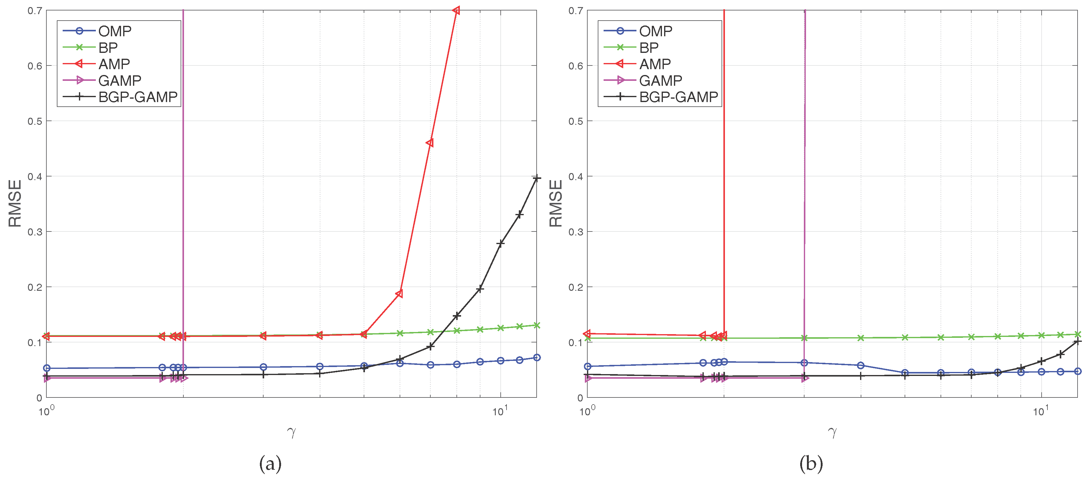
The first experiment, termed
γ test, investigates non-zero mean Gaussian sensing matrix case. We create two types of sensing matrix: type 1 means
; type 2 means
, where each entry of
is i.i.d. drawn from
. Set the range of
γ to
.
Figure 1a shows that GAMP violently diverges at
, AMP fast diverges at
. The severely sharp divergence of GAMP and AMP comes from the phase transition property of compressed sensing. Although BGP-GAMP also begins to diverge at
, the deterioration speed is slower than AMP. Furthermore, the RMSE of BGP-GAMP is always less than that of AMP. When
, the RMSE of BGP-GAMP is a little less than that of OMP, and when
, the RMSE of BGP-GAMP is obviously less than that of BP.
Figure 1b shows that AMP violently diverges at
, GAMP violently diverges at
, but BGP-GAMP just begins to diverge at
. The RMSE of BGP-GAMP is always less than that of BP, and less than that of OMP until
. Moreover,
Figure 1a,b shows that BGP-GAMP outperforms OMP slightly in performance over a parameter range
. In summary, our proposed algorithm obtains better robustness compared with the standard AMP/GAMP algorithms, at the same time our proposed algorithm achieves performance advantage over a suitable parameter range compared with the standard OMP and BP algorithms.
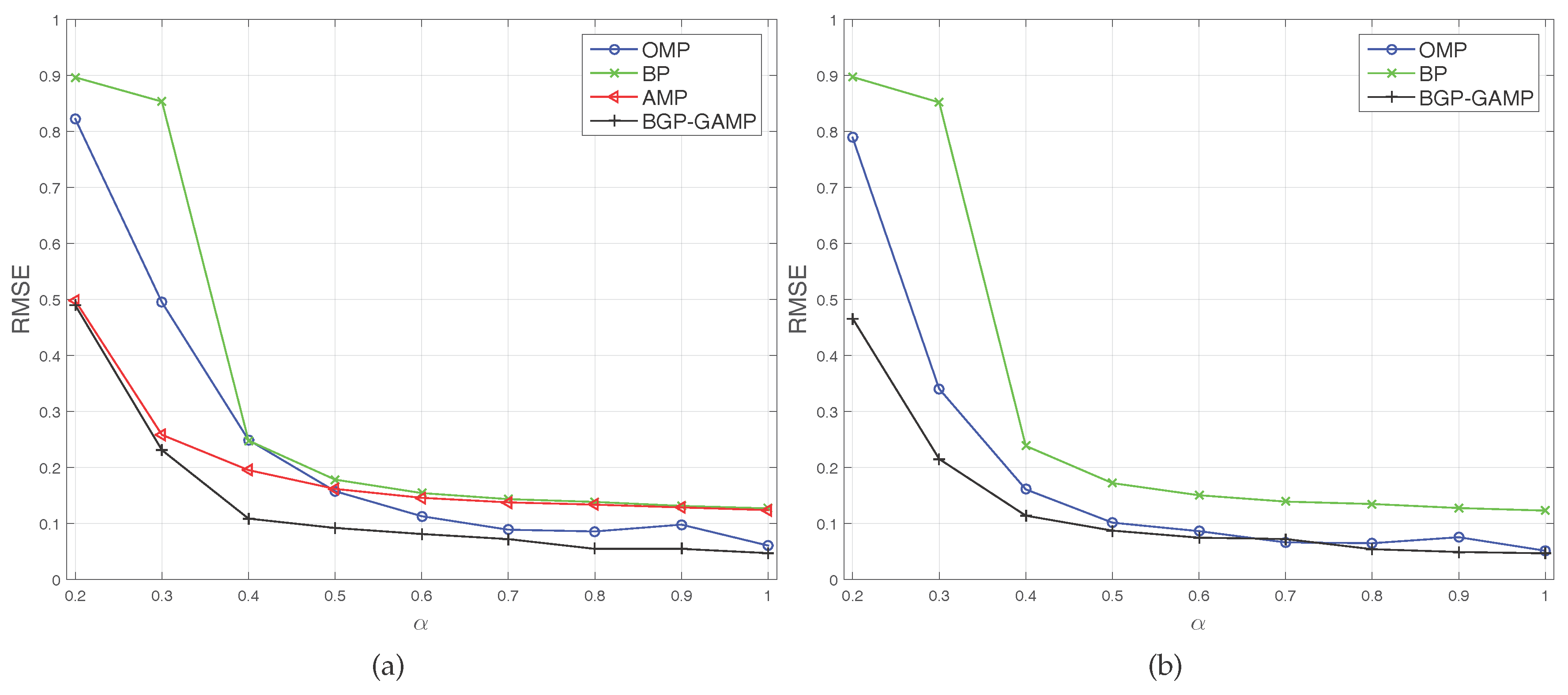
The second experiment, termed
α test, investigates the highly correlated columns sensing matrix
case. The elements of
are neither normal nor i.i.d distributed. Create two types of sensing matrix: type 1 means
, where
, and
; type 2 means
like type 1, but normalizes each column of
. We know that
is
low rank for
. Set the range of
α to
. Since GAMP totally diverges at every
α with type 1 and type 2 cases, it is not visible in
Figure 2a,b. AMP also totally diverges at every
α with type 2 case, therefore it is also not visible in
Figure 2b. The two figures show that BGP-GAMP remains stable even in a low rank scenario
, and its performance is obviously better than AMP and BP, and a little better than OMP.
It is worth noting that the threshold
in
Figure 1 and
Figure 2 is the relative mean square error, not absolute mean square error, which means the average error amplitude is just
of the original signal amplitude. These figures show, for instance, that the standard AMP algorithm and BP algorithm are approaching this threshold. Therefore, it is not a poor performance. We do not consider MAP-GAMP since MAP estimation is not general as MMSE estimation, please see [
11] Section 3.6.3 for more discussion.
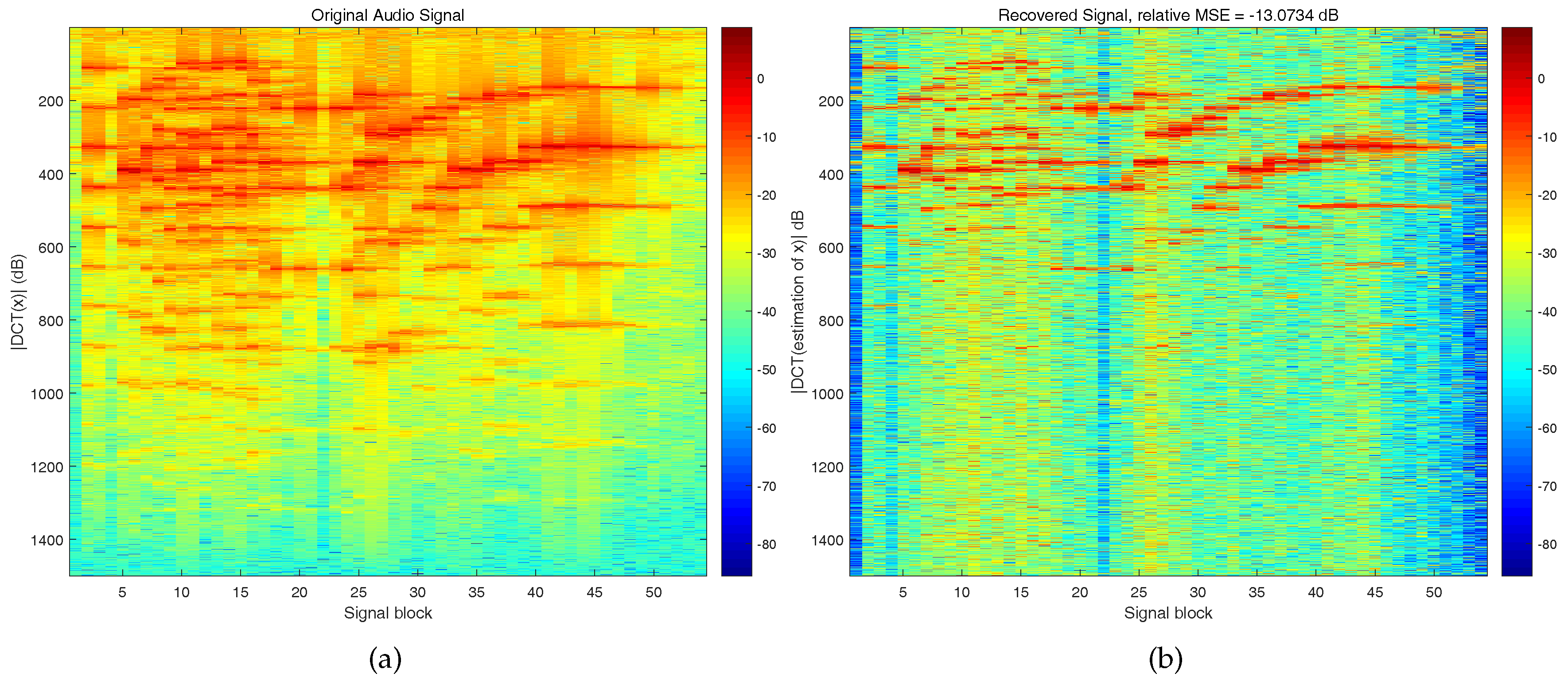
The last experiment uses real world data, namely, a segment of music by Mozart. The data has 81,000 sample points, and it is segmented to 54 blocks, each block has
sample points. The compressed sampling rate is set to
, therefore, the measurement number is
. We create the sensing matrix by DCT transform:
, where every element of Φ is drawn from
, and then multiplied a scale factor
to it.
Figure 3a shows the modulus of DCT coefficients of the original signal, and
Figure 3b shows the modulus of DCT coefficients of the recovered signal. We can see that the major energy has been recovered from the compressed measurements.


