Moving Mesh Strategies of Adaptive Methods for Solving Nonlinear Partial Differential Equations

Abstract

This paper proposes moving mesh strategies for the moving mesh methods when solving the nonlinear time dependent partial differential equations (PDEs). Firstly we analyse Huang’s moving mesh PDEs (MMPDEs) and observe that, after Euler discretion they could be taken as one step of the root searching iteration methods. We improve Huang’s MMPDE by adding one Lagrange speed term. The proposed moving mesh PDE could draw the mesh to equidistribution quickly and stably. The numerical algorithm for the coupled system of the original PDE and the moving mesh equation is proposed and the computational experiments are given to illustrate the validity of the new method.

1. Introduction

For the numerical solution of nonlinear partial differential equations (PDEs) which involve large solution variations, large curvatures and even shock waves, two kinds of methods are generally considered. One is the Eulerian method [1,2,3,4] for which the fixed mesh is employed, when the length of the shock wave is similar to the length of the mesh, the accuracy will diminish significantly. In contrast, the other method: the Lagrangian (adaptive) method [5,6] is more efficient. In this case, the mesh is moved adaptively and always concentrated in regions with large and rapid variations.

In this paper we concentrate on one kind of adaptive method: moving mesh methods. The mesh of fixed number of knots are moved according to a moving mesh equation. The original PDE and the moving mesh equation form a coupled system and are often solved simultaneously by various numerical methods. Since the moving element methods by Miller et al. [7] and the moving finite methods by Dorfi et al. [8], the moving mesh method have been under extensive study, for details we refer the reader to [6,9,10,11,12,13,14,15,16,17,18,19,20,21] and the references therein.

One important work of the moving mesh method is the formulation of an efficient moving mesh PDE. In 1974, de Boor [22] proposed the equidistribution principle (EP) which offered an excellent error estimation principle when formulating moving mesh equations. Afterwards, a mount of moving mesh PDEs were constructed directly or indirectly based on the EP [6,14,15,17,18,23]. In 1994, Huang et al. [9] summarized and constructed the one-dimensional MMPDEs based on EP. Then the moving mesh methods were extended to high dimensions [6,13,24]. Since the moving mesh methods are widely and successfully applied to practical problems [19,21,25,26], the methods have been studied extensively [6,11,12,25]. The theoretical and numerical problems regarding the constructions of proper moving mesh equations are still the subject of research [6,13,19,27,28,29].

In [6,9], Huang proposed seven kinds of location based MMPDEs based on EP, both the theoretical and numerical problems have been analysed extensively, which offer a outstanding guidance when applying these MMPDEs in the practical problems. We observed that, after Euler discretization on time, the MMPDEs could be taken as deformations of iteration methods on EP. Based on this new explanation, the convergence conditions and orders on fixed time could be obtained. Moreover, the parameter in the MMPDEs which determines the speed of the equidistribution could be estimated.

The new explanation leaves space to improve Huang’s MMPDEs by adding a velocity-based term. In 2005, Wu et al. [30,31] constructed moving mesh PDEs which move the mesh along the characteristic line of the original PDE. Wu’s methods are able to maintain the distribution of knots during time iteration.

Combining the location based method by Huang and velocity based method by Wu, we construct the moving mesh PDEs in which the mesh are moved by two steps: firstly the approximation to the EP on fixed time, then the movement along the character line of the original PDE to keep the distribution. The moving mesh PDE accelerated the convergence speed and stabilized the moving process of the mesh to the EP. Compared with the existing two methods, the proposed method is more stable and could simulate sharper and faster propagating shock waves.

The moving mesh PDE and the original PDE form a coupled PDE system [9]. In this manuscript, the PDE system is simulated simultaneously by methods of line. The system was first discretized in the spatial domain, and then the resulting system of ordinary differential equations (ODEs) is integrated using an variable step size ODE solver to observe the performance of the moving mesh equations.

The rest of the paper is organized as follows: We propose the improved moving mesh PDE in Section 2. The numerical algorithms are presented in Section 3. Section 4 shows the experiments to illustrate the validity of the new method. We end this paper with a brief conclusion in Section 5.

2. The Improved Moving Mesh PDEs

We show the approach through an example, and it can be generalized to various other kinds of the time dependent propagations problems. Consider the non-linear partial differential propagations equation:

$$u_t=L(u)u_x$$

(1)

subject to appropriate boundary and initial conditions, where L represents a differential operator involving only spatial derivatives.

Without loss of generality one can assume that $x\in [0,1]$. An one to one coordinate transformation between the computational domain and physical domain is defined as:

$$x=x(\xi ,t),\xi \in [0,1],$$

and the coordinate transformation satisfies:

$$x(0,t)=0,x(1,t)=1.$$

(2)

The EP proposed by de Boor for determine $x(\xi ,t)$ is to require equidistribution of a positive monitor function M, so that:

$$E_1(x(\xi ,t),t)\doteq {\int }_0^{x(\xi ,t)}M(x,t)dx-\xi s(t)=0,$$

(3)

where $s(t)={\int }_0^{1}M(x,t)dx$.

Although the choice of the monitor function is important for the distribution of the mesh, we will utilize the arclength monitor function $M(x)=\sqrt{1+{(u_x)}^2}$ in this manuscript.

2.1. Analysis of Huang’s MMPDEs

Huang [9] gave the differential forms of the EP:

$$\begin{array}{c}{E}_2(x(\xi ,t),t)\doteq M(x(\xi ,t),t)\frac{\partial x(\xi ,t)}{\partial \xi }-s(t)=0;\hfill \end{array}$$

(4)

$$\begin{array}{c}{E}_3(x(\xi ,t),t)\doteq \frac{\partial }{\partial \xi }(M(x(\xi ,t),t)\frac{\partial x(\xi ,t)}{\partial \xi })=0.\hfill \end{array}$$

(5)

With the boundary conditions of (2), the Equations (4) and (5) are equivalent to the EP (3).

Based on the EP (3) and its derivatives (4), (5) Huang [6,9] constructed a series MMPDEs, the typical ones of them are as follows:

$$\begin{array}{c}MMPDE3:\frac{{\partial }^2}{\partial {\xi }^2}(M{x}_t)=-\frac{1}{\tau }\frac{\partial }{\partial \xi }(M\frac{\partial x}{\partial \xi });\hfill \\ MMPDE4:\frac{\partial }{\partial \xi }(M\frac{\partial x_t}{\partial \xi })=-\frac{1}{\tau }\frac{\partial }{\partial \xi }(M\frac{\partial x}{\partial \xi });\hfill \\ MMPDE5:x_t=-\frac{1}{\tau }\frac{\partial }{\partial \xi }(M\frac{\partial x}{\partial \xi });\hfill \\ ModifiedMMPDE5:x_t=-\frac{1}{\tau M}\frac{\partial }{\partial \xi }(M\frac{\partial x}{\partial \xi });\hfill \\ MMPDE6:\frac{{\partial }^2{x}_t}{\partial {\xi }^2}=-\frac{1}{\tau }\frac{\partial }{\partial \xi }(M\frac{\partial x}{\partial \xi }).\hfill \end{array}$$

Here τ is a small parameter that determine the speed of the equidistribution of the mesh. In Huang [9], MMPDE3 and MMPDE4 are obtained from the Taylor expansion of the EP (5) with a time delay by dropping the high order terms. MMPDE5 and MMPDE6 are obtained based on the attraction and repulsion pseudoforces. Numerical and theoretical analysis about these MMPDEs are detailed in [6,11].

Here we try to propose a simple explanation of the MMPDEs in the following theorem. Compared with the source of the MMPDEs proposed in [6,9], the new explanation is more rational and direct and many theoretical problems could be settled simultaneously.

Theorem 1.

After Euler discretization on time, MMPDE 3-6 could be taken as one step of root searching iteration methods of the EPs (3),(4), or (5).

Proof of Theorem 1.

Integrating MMPDE 3,4,6 to ξ twice, and by the boundary conditions of (2), MMPDE 3-6 becomes:

$$\begin{array}{c}{x}_t=-\frac{1}{\tau }\frac{E_1(x,t)}{E_{1x}^{\prime }(x,t)},\hfill \end{array}$$

(6)

$$\begin{array}{c}{x}_t=-\frac{1}{\tau }\frac{E_1(x,t)}{E_{1x}^{\prime }(\eta ,t)},\hfill \end{array}$$

(7)

$$\begin{array}{c}{x}_t=-\frac{1}{\tau }{E}_3(x,t),\hfill \end{array}$$

(8)

$$\begin{array}{c}{x}_t=-\frac{1}{\tau }\frac{E_3(x,t)}{E_{1x}^{\prime }(x,t)},\hfill \end{array}$$

(9)

$$\begin{array}{c}{x}_t=-\frac{1}{\tau }{E}_1(x,t),\hfill \end{array}$$

(10)

separately, where $E_{1x}^{\prime }(x,t)=M(x,t)$, $\eta \in (0,x(\xi ,t))$.

Taking MMPDE 3 as one example, discreting the above Equation (6) applying the explicit Euler discretization on time, one can get:

$$x(\xi ,t_{k+1})=x(\xi ,t_k)-\frac{▵t_k}{\tau }\frac{E_1(x(\xi ,t_k),t_k)}{E_{1x}^{\prime }(x(\xi ,t_k),t_k)},$$

where $▵t_k=t_{k+1}-t_k$ is the k-th time step.

In order to interpret MMPDE 3 more precisely and observe its differences with other moving mesh equations, we divide the above equation into two steps:

$$\{\begin{array}{}(11\text{a})& x^{(1)}(\xi ,t_k)=x(\xi ,t_k)-\frac{▵t_k}{\tau }\frac{E_1(x(\xi ,t_k),t_k)}{E_{1x}^{\prime }(x(\xi ,t_k),t_k)},(11\text{b})& x(\xi ,t_{k+1})=x^{(1)}(\xi ,t_k),\end{array}$$

where $x^{(1)}(\xi ,t_k)$ is an intermediate term.

One can conclude that (11a) is one step root searching Newton iteration of EP (3) at time $t_k$ with $\frac{▵t_k}{\tau }$ as the relaxation factor. According to the theory of iteration methods, the convergence condition of MMPDE 3 on fixed time $t_k$ is

$$0<|\frac{▵t_k}{\tau M(x,t)}|<2.$$

The source of other MMPDEs could be explained similarly, the theorem is proved. ☐

New MMPDEs could be constructed similarly based on the EPs, such as:

$$\begin{array}{c}{x}_t=-\frac{1}{\tau }\frac{E_2(x,t)}{E_{2x}^{\prime }(x,t)},\hfill \end{array}$$

(12)

$$\begin{array}{c}{x}_t=-\frac{1}{\tau }\frac{E_3(x,t)}{E_{3x}^{\prime }(x,t)},\hfill \end{array}$$

(13)

$$\begin{array}{c}{x}_t=-\frac{1}{\tau }{E}_2(x,t),\hfill \end{array}$$

(14)

and their convergence conditions could be obtained similarly.

According to Theorem 1, (6) is the best, since it is a Newton iteration method derived from the original EP (3). Theorem 1 leaves a space for us to combine Huang location-based MMPDEs with the velocity based methods. Hence the convergence speed could be accelerated.

2.2. The Moving Mesh Equation Based on the Characteristic Line

Taking the original PDE (1) as a Hyperbolic PDE locally, Wu [30] let the mesh move along the characteristic line, for the original PDE (1), Wu [30]’s moving mesh equation is:

$$u_t=-L(u),$$

(15)

which is the direction of character line of the original PDE (1).

Discreting Equation (15) applying the explicit Euler discretization on time, one can get:

$$x(t_{k+1})=x(t_k)-▵t_{k}L(u(x(t_k),t_k)),$$

in order to interpret the moving mesh Equation (15) more precisely and do comparisons with other moving mesh methods, we divide the above into two steps:

$$\{\begin{array}{}(16\text{a})& x^{(1)}(t_k)=x(t_k),(16\text{b})& x(t_{k+1})=x^{(1)}(t_k)-▵t_{k}L(u(x(t_k),t_k)),\end{array}$$

where $x^{(1)}(\xi ,t_k)$ is an intermediate term.

As a velocity-based mesh movement method, Wu’s moving mesh equation takes the moving of the knots to be leaves on the wave (PDE) and the mesh is gone with the wave (PDE). The method keeps the mesh’s distribution on the solution according to time iteration. The benefit of the method is it considers the influence of the original PDE on the moving of the mesh. However, the method is not able to do the equidistribution on fixed time, if the initial mesh is not equidistributed, the mesh will always be unequidistributed until the end.

2.3. The Proposed Moving Mesh Equations

According to the discretization forms of the moving mesh equations of Huang and Wu, one can observe that Huang’s MMPDEs and Wu’s moving mesh equations are complementary. In order to accelerate the mesh’s convergence to the EP, we combine the location-based and velocity-based method and construct the new moving mesh PDE that moves the mesh by two steps: Firstly, the approximation to the EP on fixed time, then the movement along the original PDE to keep the distribution.

For the original PDE (1), the proposed moving mesh PDE takes the form:

$$x_t=-\frac{1}{\tau }\frac{E_1(x,t)}{M(x,t)}-L(u).$$

(17)

To interpret the proposed moving mesh Equation (17) more precisely, discreting Equation (17) applying the explicit Euler discretization on time, one can get:

$$x(\xi ,t_{k+1})=x(\xi ,t_k)-\frac{\Delta t_k}{\tau }\frac{E_1(x(\xi ,t_k),t_k)}{E_{1x}^{\prime }(x(\xi ,t_k),t_k)}-▵t_{k}L(u(x(\xi ,t_k),t_k)),$$

divide the above into two steps:

$$\{\begin{array}{}(18\text{a})& x^{(1)}(\xi ,t_k)=x(\xi ,t_k)-\frac{\Delta t_k}{\tau }\frac{E_1(x(\xi ,t_k),t_k)}{E_{1x}^{\prime }(x(\xi ,t_k),t_k)},(18\text{b})& x(\xi ,t_{k+1})=x^{(1)}(\xi ,t_k)-▵t_{k}L(u(x(\xi ,t_k),t_k)),\end{array}$$

where $x^{(1)}(\xi ,t_k)$ is an intermediate term.

Remark 1.

For arbitrary initial mesh, if the mesh is already equidistributed, $E_1=0$, (18a) is no longer in force and (18b) keeps the equidistribution when moved to the next time iteration. If the mesh is not equidistributed, then $E_1\ne 0$, (18a) could draw the mesh to be more equidistributed, then (18b) could keep the distribution when moved to the next time iteration. For arbitrary initial mesh, the new moving mesh PDE is able to draw the mesh to equidistribution efficiently and stably.

Remark 2.

Compared with the semi-discretization of moving mesh PDEs (11) proposed by Huang, (16) proposed by Wu, and the present (18), one can observe that the proposed moving mesh equation includes both the advantages of the MMPDEs proposed by Huang and Wu. The convergence speed of the mesh to the EP are accelerated and the mesh equidistribution process is more continuous, hence, the probability of the mesh crossing during time iterations is reduced, and the moving mesh process becomes more stable.

3. The Numerical Algorithms

Using the coordinate transformation, (1) can be rewritten as:

$$u_t-u_x{x}_t=L(u)u_x,$$

(19)

Equations (17) and (19) form a coupled PDE system, and it could be simulated by various numerical methods, such as the finite difference method [20], the finite element method [14], the meshfree methods [30,31] and so forth. In this manuscript, we apply the method of line in Huang [6,9] for the numerical solution of the system to compare the proposed moving mesh PDE with Huang’s MMPDEs. Specifically, the PDEs are first discretized in the spatial domain and then the resulting system of ODEs is integrated using an ODE solver.

Discreting the PDE system applying central finite differences, for $j=1,\cdots ,N-1$, one can get:

$$\begin{array}{c}\frac{d{u}_j}{dt}-\frac{u_{j+1}-u_{j-1}}{x_{j+1}-x_{j-1}}\frac{d{x}_j}{dt}=L(u_j)\frac{u_{j+1}-u_{j-1}}{x_{j+1}-x_{j-1}},\hfill \end{array}$$

(20)

$$\begin{array}{c}\frac{d{x}_j}{dt}=-\frac{1}{▵t}\frac{E_{1,j}}{M_j}-L(u_j),\hfill \end{array}$$

(21)

where the integration $E_1$ is approximated applying the trapezoidal method,

$$\begin{array}{c}{M}_j=\sqrt{1+{(\frac{u_{j+1}-u_{j-1}}{x_{j+1}-x_{j-1}})}^2},\hfill \\ E_{1,j}=\sum _{i=1}^j\frac{M_i+M_{i-1}}{2}(x_i-x_{i-1})-\frac{j}{N}\sum _{i=1}^N\frac{M_i+M_{i-1}}{2}(x_i-x_{i-1}),\hfill \end{array}$$

$u_j(t)\approx u(x({\xi }_j,t),t),x_j(t)=x({\xi }_j,t),{\xi }_j=\frac{j}{N},j=0,1,\cdots ,N$. The expression of $L(u_j)$ depends on its specific form.

When applying (17) in the practical problems, to avoid mesh crossing and keep the mesh moving stably, the spatial smoothing techniques proposed in [11] are employed; when treating the boundary nodes in the Lagrange method, the technique in [30] is applied.

Equations (20) and (21) form an ODE system, the system could be simulated by various schemes, such as the upwinding differencing. In this manuscript, the system is simulated using a MATLAB ODE solver “ode15i” as in [6] in order to observe the performances of the moving mesh PDEs. The method use a variable step-size backward differentiation Runge–Kutta schemes of order 5 and the method selects the step size based on the accuracy of the solution [32]. The required input data is the initial and boundary conditions, the output time, the numberer of the knots N and local time stepping tolerance $atol$ and $rtol$. Throughout in this paper we set

$$N=21,atol={10}^{-4},rtol={10}^{-5}.$$

4. Experiments

In this section, the numerical results are presented for the moving mesh methods. One example is the well known convection diffusion equation, the other example is the Burgers equation. We choose these problems as our test examples because they have been used extensively in the adaptive methods literature. It is worth emphasizing that these problems are also the ones used in [6,9,29,30,33].

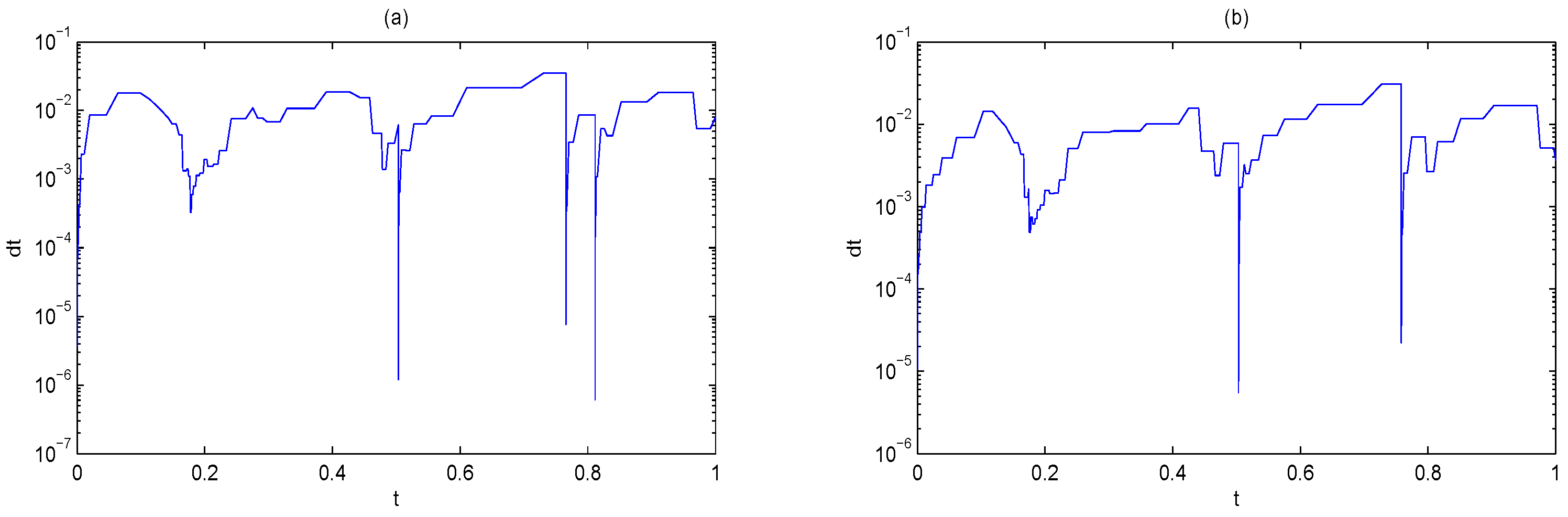
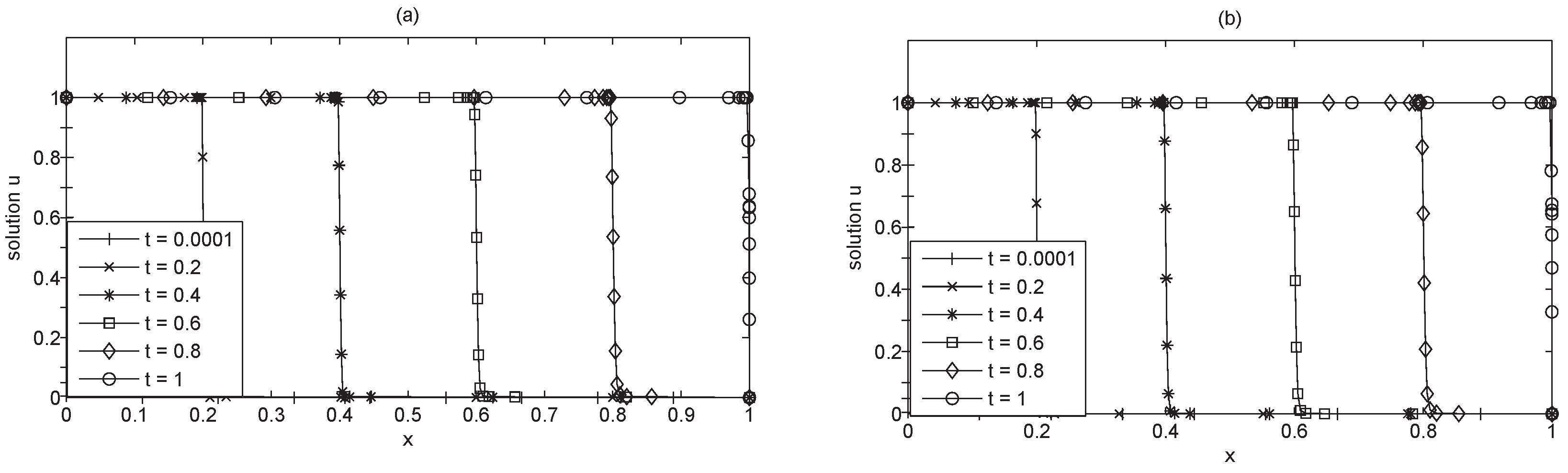
4.1. Advection-Diffusion Equation

The first example is the advection-diffusion equation

$$u_t=ϵu_{xx}-V\frac{\partial u}{\partial x},x\in (0,1),$$

(22)

where $ϵ>0$ is the diffusion coefficient, and V is the flow velocity. Let $ϵ={10}^{-5}$, $V=1$ and Dirichlet boundary conditions at the endpoints $x=0$ and $x=1$ are chosen such that the exact solution is:

$$u(x,t)=\frac{1}{2}erfc(\frac{x-t}{\sqrt{4ϵt}})+\frac{1}{2}exp(\frac{x}{ϵ})erfc(\frac{x+t}{\sqrt{4ϵt}}),$$

where $erfc(x)$ is the complementary error function. The smaller ϵ, the steeper the traveling front.

The exact solution is singular at $t=0$. The integration starts at $t=0.0001$ and stops at $t=1$, when the steep front reaches the right endpoint.

Figure 1 and Figure 2 are the results of the two methods. One can observe from Figure 1 that both the two methods perform similarly. However, Figure 2 shows that Huang’s method are less stable than the proposed method. The time step sizes of the proposed method are larger and smoother, which results in less consuming time and iterations, as is shown in

Table 1. The comparison of computational time and iterations of Huang’s method and the proposed method for different examples.

	Huang’s method		The Proposed Method
	Computational Time (s)	Iterations	Computational Time (s)	Iterations
Advection-diffusion equation	2.47354	664	1.86607	279
Burgers equation with $n=1$	1.11280	258	0.89543	254
Burgers equation with $n=10$	4.6116	1236	2.43196	1154
Burgers equation with $n=20$	4.85784	2205	4.14323	2008
Burgers equation with $n=25$	8.48143	23,014	8.05290	8837
Burgers equation with $n=30$	70.785286	30,167	15.54634	13,053

.

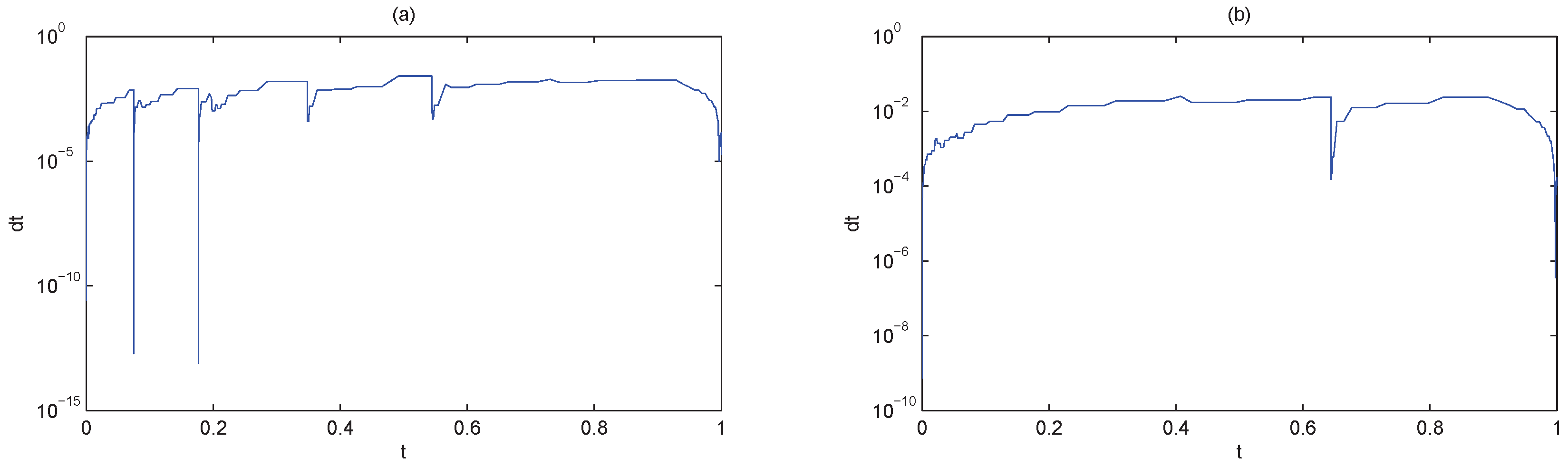
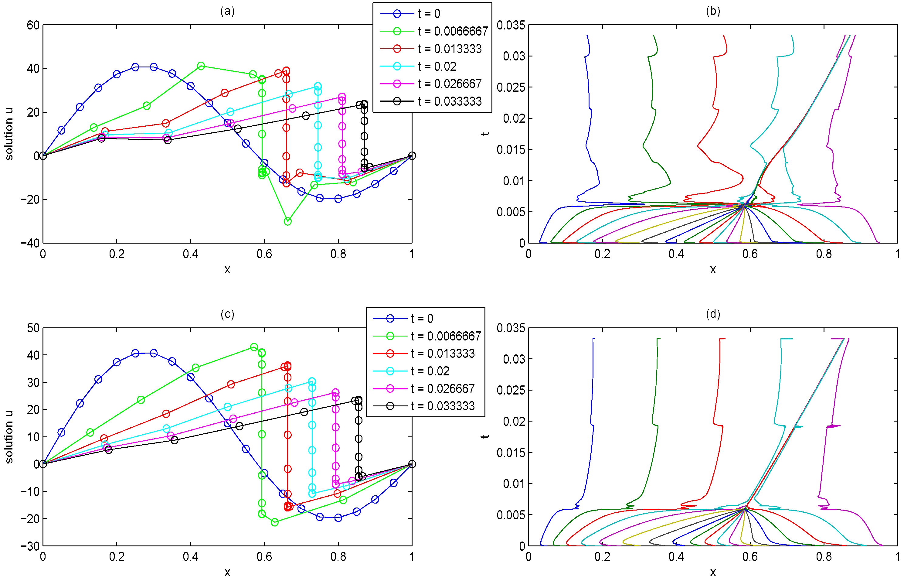
4.2. Burgers Equation

For the Burgers equation:

$$u_t=ϵu_{xx}-{(\frac{u^2}{2})}_x,x\in (0,1),$$

(23)

subject to the boundary conditions:

$$u(0,t)=u(1,t)=0,$$

(24)

and initial conditions:

$$u(x,0)=nsin(2\pi x)+0.5nsin(\pi x),$$

(25)

where n is a constant and $ϵ={10}^{-5}$, the solution has a smooth initial profile and develops a steep front. For different n, the front grows to n times higher and propagates toward the right end and eventually dies out at $t=\frac{1}{n},x=1$ which is n times quicker than $n=1$. The difficulty with the numerical solution of the problem is the resolution of this propagating steep front.

For Burgers Equations (23)–(25) with $n=1$, Figure 3 shows the numerical solutions and the trajectories applying Huang’s methods (modified MMPDE5) and the proposed method. Both the two methods simulate the Burgers Equation precisely in a short time and the trajectories are smooth. The advantage of the new method is not valid. Figure 4 shows the time step sizes of the two methods. It is possible to determine from this that, for the same accuracy, the time step sizes of the proposed method are larger than Huang’s methods, which means that the proposed method consumes less time and iterations when simulating the Burgers equation.

When $n=30$, according to the above analysis, the solution grows to 30 times of $n=1$ and the shock wave propagates to the end at time $t=\frac{1}{30}$ (about $0.033$). As is shown in Figure 5, from the solutions applying the Huang’s method bad nodes emerge, and the trajectories begin to be rough and unstable. Figure 6 shows that, for the same accuracy, the time step sizes of Huang’s method are smaller than the proposed method. As a result, Huang’s method consumes more time and iterations. However, the proposed method could simulate the PDE more efficiently and stably.

Table 1 shows the computational time and iteration times of the Burgers equation applying 21 knots with different n . One can observe that when n is small, the two methods’ computational time and iterations are similar, as n grows, the modified MMPDE 5 spends more time and yields much more time iterations than the proposed methods. When $n=30$, the Computational time and iteration times of the proposed method is no more than $\frac{1}{4}$ of Huang’s method. From the figures and table above, the knots move steadily applying the new method, this corresponds to the analysis of Section 2.

5. Conclusions

In this paper, we construct one moving mesh equation for adaptive numerical methods when solving nonlinear PDEs. Firstly, we introduce the well known Huang’s MMPDEs. We discover that after Euler discretization, Huang’s MMPDEs could be taken as one step of root searching iteration methods of the EP or its derivatives. Secondly, we Improve Huang’s MMPDEs by adding one term which moves the mesh along the characteristic line of the original PDE. The convergence speed is accelerated and the moving mesh processes are more stable. The numerical algorithms are presented for the coupled system of the original PDE and the moving mesh PDE. We take the Advection-Diffusion equation and the Burgers equation as the examples, the method could also be applied to other time-dependent PDEs. The experiments show the validity of the proposed method.

References

1. Meis, T.; Marcowitz, U. Numerical Solution of Partial Differential Equations; Springer: New York, NY, USA, 2012. [Google Scholar]
2. Gutierrez, J.M. Numerical Properties of Different Root-Finding Algorithms Obtained for Approximating Continuous Newton’s Method. Algorithms 2015, 8, 1210–1218. [Google Scholar] [CrossRef]
3. Ullah, M.Z.; Ahmad, F.; Serra-Capizzano, S. Constructing Frozen Jacobian Iterative Methods for Solving Systems of Nonlinear Equations, Associated with ODEs and PDEs Using the Homotopy Method. Algorithms 2016, 9, 18. [Google Scholar]
4. Gao, Q.J.; Wu, Z.M.; Zhang, S.G. Applying multiquadric quasi-interpolation for boundary detection. Comput. Math. Appl. 2011, 62, 4356–4361. [Google Scholar] [CrossRef]
5. Liseikin, V.D. Grid Generation Methods; Springer: New York, NY, USA, 2009. [Google Scholar]
6. Huang, W.; Russell, R.D. Adaptive Moving Mesh Methods; Springer: New York, NY, USA, 2011. [Google Scholar]
7. Miller, K.; Miller, R.N. Moving finite elements. I. SIAM J. Numer. Anal. 1981, 18, 1019–1032. [Google Scholar] [CrossRef]
8. Dorfi, E.A.; Drury, L.O.C. Simple adaptive grids for 1-D initial value problems. J. Comput. Phys. 1987, 69, 175–195. [Google Scholar] [CrossRef]
9. Huang, W.Z.; Ren, Y.; Russell, R.D. Moving mesh partial differential equations (MMPDEs) based on the equidistribution principle. SIAM J. Sci. Comput. 1994, 31, 709–730. [Google Scholar] [CrossRef]
10. Budd, C.J.; Huang, W.; Russell, R.D. Moving mesh methods for problems with blow-up. SIAM J. Sci. Comput. 1996, 17, 305–327. [Google Scholar] [CrossRef]
11. Huang, W.Z.; Russell, R.D. Analysis of moving mesh partial differential equations with spatial smoothing. SIAM J. Numer. Anal. 1997, 34, 1106–1126. [Google Scholar] [CrossRef]
12. Huang, W. Practical aspects of formulation and solution of moving mesh partial differential equations. J. Comput. Phys. 2001, 171, 753–775. [Google Scholar] [CrossRef]
13. Li, R.; Tang, T.; Zhang, P. Moving mesh methods in multiple dimensions based on harmonic maps. J. Comput. Phys. 2001, 170, 562–588. [Google Scholar] [CrossRef]
14. Li, R.; Tang, T.; Zhang, P. A moving mesh finite element algorithm for singular problems in two and three space dimensions. J. Comput. Phys. 2002, 177, 365–393. [Google Scholar] [CrossRef]
15. Tan, Z.; Zhang, Z.; Huang, Y.; Tang, T. Moving mesh methods with locally varying time steps. J. Comput. Phys. 2004, 200, 347–367. [Google Scholar] [CrossRef]
16. Tang, T. Moving mesh methods for computational fluid dynamics. Contemp. Math. 2005, 383, 141–174. [Google Scholar]
17. Tang, H.Z. A moving mesh method for the Euler flow calculations using a directional monitor function. Commun. Comput. Phys. 2006, 1, 656–676. [Google Scholar]
18. Yao, J.; Liu, G.R.; Qian, D.; Chen, C.-L.; Xu, G.X. A moving-mesh gradient smoothing method for compressible CFD problems. Math. Mod. Meth. Appl. Sci. 2013, 23, 273–305. [Google Scholar] [CrossRef]
19. Browne, P.A.; Budd, C.J.; Piccolo, C.; Cullen, M. Fast three dimensional r-adaptive mesh redistribution. J. Comput. Phys. 2014, 275, 174–196. [Google Scholar] [CrossRef]
20. Lee, T.E.; Baines, M.J.; Langdon, S. A finite difference moving mesh method based on conservation for moving boundary problems. J. Comput. Appl. Math. 2015, 288, 1–17. [Google Scholar] [CrossRef]
21. Lu, C.; Huang, W.; Qiu, J. An Adaptive Moving Mesh Finite Element Solution of the Regularized Long Wave Equation. 2016; arXiv:1606.06541. [Google Scholar]
22. De Boor, C. Good Approximation by Splines with Variable Knots, II. In Conference on the Numerical Solution of Differential Equations; Springer: Heidelberg/Berlin, Germany, 1974. [Google Scholar]
23. Budd, C.J.; Huang, W.; Russell, R.D. Adaptivity with moving grids. Acta Numer. 2009, 18, 111–241. [Google Scholar] [CrossRef]
24. Huang, W.; Russell, R.D. Moving mesh strategy based on a gradient flow equation for two-dimensional problems. SIAM J. Sci. Comput. 1998, 20, 998–1015. [Google Scholar] [CrossRef]
25. Huang, W.; Kamenski, L. A geometric discretization and a simple implementation for variational mesh generation and adaptation. J. Comput. Phys. 2015, 301, 322–337. [Google Scholar] [CrossRef]
26. Luo, D.; Huang, W.; Qiu, J. A hybrid LDG-HWENO scheme for KdV-type equations. J. Comput. Phys. 2016, 313, 754–774. [Google Scholar] [CrossRef]
27. Ngo, C.; Huang, W. A Study on Moving Mesh Finite Element Solution of the Porous Medium Equation. 2016; arXiv:1605.03570. [Google Scholar]
28. Ong, B.; Russell, R.; Ruuth, S. An hr Moving Mesh Method for One-Dimensional Time-Dependent PDEs. In Proceedings of the 21st International Meshing Roundtable; Springer: Berlin/Heidelberg, Germany, 2013; pp. 39–54. [Google Scholar]
29. Uzunca, M.; Karasozen, B.; Kucukseyhan, T. Moving Mesh Discontinuous Galerkin Methods for PDEs with Traveling Waves. Appl. Math. Comput. 2017, 292, 9–18. [Google Scholar] [CrossRef]
30. Wu, Z.M. Dynamical knot and shape parameter setting for simulating shock wave by using multi-quadric quasi-interpolation. Eng. Anal. Bound. Elem. 2005, 29, 354–358. [Google Scholar] [CrossRef]
31. Zhu, C.G.; Wang, R.H. Numerical solution of Burgers’ equation by cubic B-spline quasi-interpolation. Appl. Math. Comput. 2009, 208, 260–272. [Google Scholar] [CrossRef]
32. Hairer, E.; Wanner, G. Solving Ordinary Differential Equations. II; Springer: New York, NY, USA, 1991. [Google Scholar]
33. Soheili, A.R.; Kerayechian, A.; Davoodi, N. Adaptive numerical method for Burgers-type nonlinear equations. Appl. Math. Comput. 2012, 219, 3486–3495. [Google Scholar] [CrossRef]
Figure 1. Numerical solutions of Advection-diffusion equation applying Huang’s method (a) and the proposed method (b), N = 21.
Algorithms 09 00086 g001
Figure 2. The time step size for the Advection-diffusion equation with Huang’s method (a) and the proposed method (b), N = 21.
Algorithms 09 00086 g002
Figure 3. Numerical solutions and trajectories of the Burgers equation with n = 1 applying Huang’s method (a,b) and the proposed method (c,d).
Algorithms 09 00086 g003
Figure 4. The time step sizes for Burgers equation with n = 1 applying Huang’s method (a) and the proposed method (b).
Algorithms 09 00086 g004
Figure 5. Numerical solutions and trajectories of Burgers equation with n = 30 applying Huang’s method (a,b) and proposed method (c,d).
Algorithms 09 00086 g005
Figure 6. The time step sizes for Burgers equation with n = 30 applying Huang’s method (a) and the proposed method (b).
Algorithms 09 00086 g006