
Which, When, and How: Hierarchical Clustering with Human–Machine Cooperation


Computer and Information Sciences, Temple University, PA 19121, USA
*
Author to whom correspondence should be addressed.
Algorithms 2016, 9(4), 88; https://doi.org/10.3390/a9040088
Submission received: 3 November 2016
/
Revised: 13 December 2016
/
Accepted: 14 December 2016
/
Published: 21 December 2016
Abstract
:Human–Machine Cooperations (HMCs) can balance the advantages and disadvantages of human computation (accurate but costly) and machine computation (cheap but inaccurate). This paper studies HMCs in agglomerative hierarchical clusterings, where the machine can ask the human some questions. The human will return the answers to the machine, and the machine will use these answers to correct errors in its current clustering results. We are interested in the machine’s strategy on handling the question operations, in terms of three problems: (1) Which question should the machine ask? (2) When should the machine ask the question (early or late)? (3) How does the machine adjust the clustering result, if the machine’s mistake is found by the human? Based on the insights of these problems, an efficient algorithm is proposed with five implementation variations. Experiments on image clusterings show that the proposed algorithm can improve the clustering accuracy with few question operations.
1. Introduction
Researchers in Human–Computer Interaction (HCI) have made substantial breakthroughs in the field of cognitive science. HCI [1,2,3] focuses on the concept that the human instructs the machine to accomplish the computational task. In contrast, the latest research sheds light on a novel method called Human–Machine Cooperation (HMC) [4,5,6,7], where the machine dominates the computation process with limited help from the human. HMC aims to balance the advantages and disadvantages of human computation (accurate but costly) and machine computation (cheap but inaccurate).
This paper rethinks the hierarchical clustering with HMC and validates this approach in image clustering applications, including plant species clusterings and face clusterings [8]: (1) plant species clusterings aim to group leaf images by species. However, accurate clustering may require human experience (depending on the application), leading to an overly large amount of human computations. To reduce the amount of human computations, the machine can preliminarily cluster the leaf images, using existing approaches that measure the similarity of two leaf images. While automatic clusterings for leaf images are quite noisy [9], we observe that even a person can compare two leaf images and provide an accurate assessment of their similarity. Therefore, HMCs are valuable; and (2) in surveillance videos, real-time face clusterings are critical for determining whether the same person has visited a number of locations or not. Video images have variations in pose, illumination and resolution, and thus automatic clusterings are quite error-prone. However, a person can readily look at two face images to determine their similarity. Therefore, HMCs are also valuable.
We mainly focus on the HMC-based agglomerative hierarchical clusterings, and we assume that the distances between pairs of data points are known a priori. Traditional approaches without HMCs start by treating each data point as a singleton cluster, and then repeatedly merge the two closest clusters until a stop criterion is met. An inefficient HMC strategy could be a sequential approach: (1) the machine first computes some complete clustering results, through using different merging criteria; (2) then, the human picks out the most correct one as the final result. A better HMC strategy that takes less time and human computation involves real-time cooperations. When the machine encounters an uncertain pair of data points in the middle of the cluster-building process, it can ask for human help through question operations. Then, the human would tell the machine whether that pair of data points are in the same cluster or not. The number of questions a machine can ask is limited by a fixed budget, due to the cost of human computations. We are interested in the machine’s strategy on handling the question operations, which is challenging in terms of three problems (“which”, “when”, and “how”).
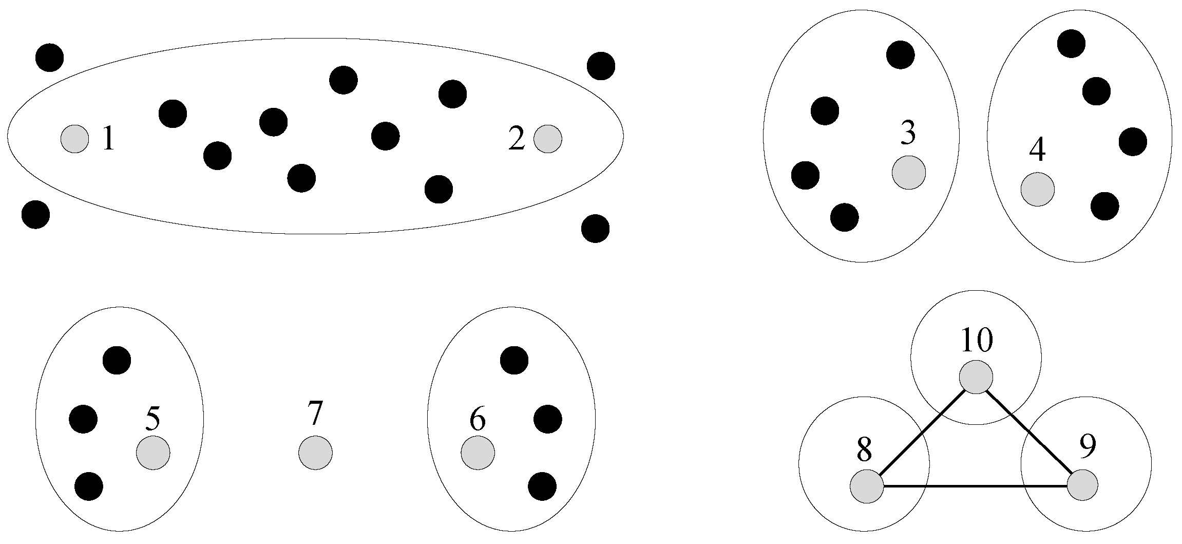
Which question (i.e., pair of data points) should the machine ask? Suppose the machine is in the middle of the cluster-building process. Then, Figure 1 shows some interesting cases as follows: (1) data points 1 and 2 are currently in the same cluster, but the distance between them is large. Hence, the machine may want human assistance to check their assignment; (2) data points 3 and 4 are currently in different clusters, but the distance between them is small. These two clusters that contain 3 and 4 may merge into a larger one; (3) the data point 7 is in the middle of two clusters. The machine can decide whether to add 7 to 5’s cluster or 6’s cluster, by asking the human two questions. Moreover, this problem is further complicated, due to the transitive relations of questions. As shown in Figure 1, let us assume that two questions return answers (from the human) in which data points 8 and 10 (the first question’s answer), as well as 9 and 10 (the second question’s answer), are in the same cluster. Based on these answers, the machine can derive that 8 and 9 are in the same cluster by transitivity.
When should the machine ask the question? Asking a question can bring up the correctness of the clustering result, since the machine may have made some errors. If the machine asks questions in the early clustering stage, then it benefits from getting a good start (or foundation) as a trade-off on the risk: it may not reserve enough question operations for very hard decisions that may appear later. The number of available questions is important: if the machine holds a large number of available questions, then it can be aggressive (i.e., ask early); otherwise, it may be conservative (i.e., ask later).
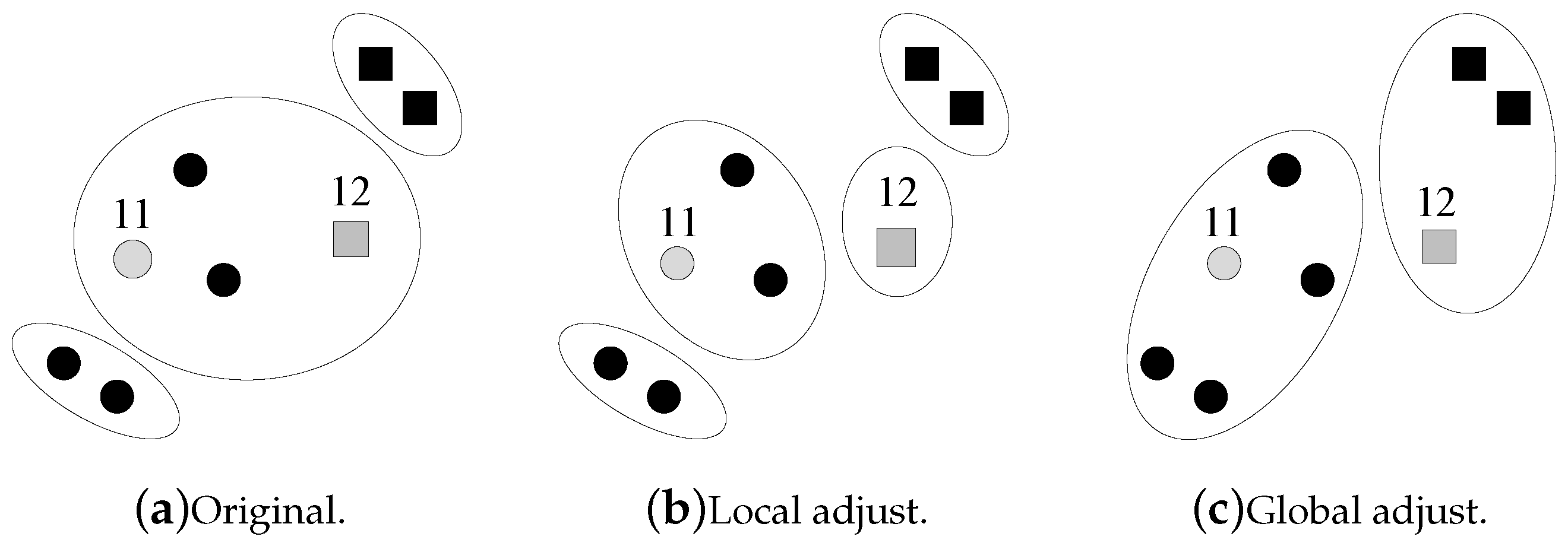
How does the machine adjust the current clustering result after obtaining the question’s answer from the human? If the human agrees with the machine’s clustering result, then everything is fine. Otherwise, the machine needs to adjust its clustering result, which is very complex due to the coupled errors shown in Figure 2. Figure 2a shows the current clustering result of the machine. Then, the machine asks a question on data points 11 and 12, and the human returns an answer that 11 and 12 are not in the same cluster. This answer brings a different clustering result, as shown in Figure 2c. Instead of locally splitting the cluster that contains 11 and 12 into two smaller clusters, the machine may need a global adjustment on the current clustering result.
Moreover, the problems of “which”, “when”, and “how” are not independent of each other. To solve the “when” problem, the machine needs to estimate the benefit brought by asking a question (as to balance the risk). Hence, the “when” problem is highly related to the “which” problem, since the machine should select the most beneficial pair of data points to ask. Meanwhile, the “how” problem is also related to the “which” problem, since the selected pair of data points may have an influence on the adjustment strategy (local or global). This paper explores the insights of these problems as our key contributions. We propose insightful solutions to the problems of “which”, “when”, and “how”.
The paper is organized as follows. We present the framework in Section 2. Related works are described in Section 3. The problems of “which”, “when”, and “how” are studied in Section 4. Section 5 gives out an overview of the proposed algorithm. Experiments are conducted in Section 6. Finally, in Section 7, we conclude the paper.
2. Algorithm Framework
2.1. Application Background
The application background of this paper comes from the image clusterings, such as plant species clusterings and face clusterings [8]:
- Plant species clusterings aim to group leaf images by species. This application requires an overly large amount of human computations, since accurate labeling needs human experience. To reduce the amount of human computations, the machine can preliminarily cluster the leaf images, based on the existing algorithms. While automatic clusterings for leaf images are quite noisy [9], we observe that even a person can compare two leaf images and provide an accurate assessment of their similarity. Therefore, HMCs are valuable.
- In surveillance videos (with the purpose of managing or protecting people), real-time face clusterings are important for determining whether the same person has visited a number of locations or not. Images from videos have variations in pose, illumination and resolution, and thus automatic clusterings are quite error-prone. However, a person can easily determine the similarity of two face images. Therefore, HMCs are also valuable.
2.2. Traditional Algorithm
As shown in Algorithm 1, the traditional agglomerative hierarchical clustering is a bottom-up approach, where each data point starts in its own cluster. Then, the two closest clusters are iteratively merged, as one moves up the hierarchy. Here, we use the MAX merging strategy [10], which defines the distance of two clusters as the distance between the furthest two data points that are respectively in these two clusters. Other merging strategies are also feasible. We denote the process of merging the two closest clusters as a clustering step. When one clustering step is executed, we say that the clustering hierarchy moves up by one. The clustering hierarchy can be measured by the number of remaining clusters (a smaller number indicates a higher clustering hierarchy). Finally, we use N to denote the total number of data points in the clustering algorithm.
| Algorithm 1: Agglomerative Hierarchical Clustering. |
| Data: Distances between pairs of data points. |
| Result: The clustering result. |
 |
2.3. Our Approach
We want to improve the accuracy of the agglomerative hierarchical clustering by HMCs, where the untrained machine acts as the dominant task solver. The machine can get limited help, in terms of question operations, from the trained human. The question operation has the format of comparing two data points (i.e., two images), since it serves as a basic unit that takes minimal human computations. For example, comparisons among three data points can be regarded as three sets of comparisons between two data points. The number of question operations is limited, since human computations are costly. We study the machine’s strategy on handling the question operations, in terms of “which”, “when”, and “how”.
Algorithm 2 shows our framework, in which lines 4, 5, and 6 represent the machine’s strategy on handling the questions. Line 4 corresponds to the “when” problem (When should the machine ask the question?); Line 5 shows the “which” problem (Which pair of data points should the machine ask?); Line 6 is the “how” problem (How does the machine adjust the current clustering result?). For simplicity, two assumptions are made as follows: (1) the machine is untrained, and thus it may make the wrong decisions during the clustering process. Meanwhile, the machine can ask the human to judge whether two data points are in the same cluster or not. We assume that the human is trained, and thus his/her judgement is always correct; and (2) we assume that the human answers a question instantaneously, i.e., there is no extra waiting time for answers.
| Algorithm 2: Our Framework. |
| Data: Distances between pairs of data points; The number of available questions. |
| Result: The clustering result |
 |
Our approach is tolerant of data noise, compared to traditional agglomerative hierarchical clustering [11]. This is because HMC is likely to fix partial problems caused by the data noise. Even if data points are incorrectly clustered, the human could help the machine to fix its error. However, the objective of our approach is not the clustering robustness under noise, meaning that the data noise problem still remains in some extreme cases. One of our future directions could be using humans to mitigate the data noise problem for clusterings.
3. Related Work
Recently, combining human and machine intelligence in crowdsourcing [12] has become a hot research area. When the machine cannot solve its task, it can ask for human help. The machine takes the part of the job that it can understand, while passing the incomprehensible part to the human. Crowdsourcing acts as the bridge that connects the machine and the human. The question response time is reported to be low enough, which provides the possibility for real-time HMCs [13]. While researchers [8,12] studied different kinds of HMC problems, we mainly focus on real-time HMCs in hierarchical clusterings [14,15].
Our work is related to the active learning techniques [16,17,18,19]. The key idea behind active learning is that a machine learning algorithm can achieve a better accuracy with fewer training labels if it is allowed to choose the data from which it learns [19]. An active learner may pose queries, usually in the form of asking the human to label unlabeled data instances. Active learning is a special case of semi-supervised learning [20,21], while our clustering problem is unsupervised. Our problem is a dynamic one that involves time; this differs from active learning, which is static. Our approach is a special time-sensitive density-weighted uncertainty-sampling-based active learning method.
Our approach can be classified as a hybrid approach of the constraint-based clustering and the budgeted learning. The constraint-based clustering [22,23,24,25,26] is initialized with pre-given constraints before executing the clustering algorithm, while our approach dynamically introduces the constraints (i.e., question answers) within the algorithm execution. We also study the time to introduce the constraint, which is represented by the “when” problem. On the other hand, although the budgeted learning [27,28,29,30] focuses on the time for the machine to learn the samples, it does not consider the clustering constraints. Our problem is a special budgeted and constrained clustering.
Our work is also related to the cognitive science field. For example, Roads et al. [5] improved image classifications with HMC via cognitive theories of similarity. Given a query image and a set of reference images, individuals are asked to select the best matching reference. Based on the similarity choice, a predictive model was developed to optimize the selection of reference images, using the existing psychological literature. Chang et al. [6] developed Alloy, which is a hybrid HMC approach to efficiently search for global contexts in crowdsourcing. Alloy supports greater global context through a new “sample and search” crowd pattern, which changes the crowd’s task from classifying a fixed subset of items to actively sampling and querying the entire dataset. Böck et al. [31] summarized user behaviors to improve the efficiency of HMC. Multimodal user behaviors (such as characteristics, emotions and feelings) are analyzed for the machine’s algorithm design.
4. “Which”, “When”, and “How”
This section explores the solutions for the “which”, “when”, and “how” problems, respectively.
4.1. The “Which” Problem
For the “which” problem, a previous work [8] proposed that the machine should ask the pair of nodes leading to a quick convergence, which does not improve the clustering accuracy. However, the goal of HMCs is to balance the advantages and disadvantages of human computation and machine computation. The former method is accurate but costly, while the latter one is cheap but inaccurate. Therefore, using human resources to save the machine’s computations is meaningless in HMCs. Our objective is to improve the machine’s clustering accuracy with limited real-time help from humans. To better explain our idea, several definitions [32] are introduced as follows.
Definition 1.
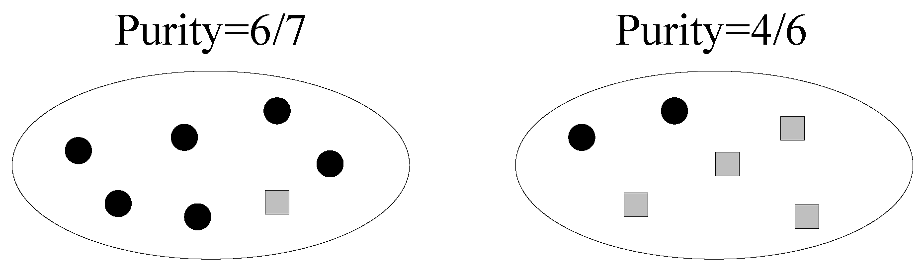
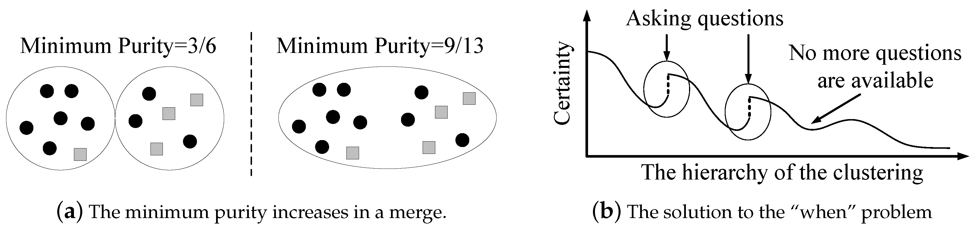
The purity of a cluster is the fraction of the dominant data point type in it. The minimum purity is the minimum purity among all clusters. The cluster with the minimum purity is called the dirtiest cluster.
Note that the definition of the minimum purity does not involve the cluster size. Therefore, a smaller cluster is more likely to have a lower purity, since an incorrectly clustered data point takes a larger fraction in the cluster. We intend to make small clusters pure, in order to limit error propagations. An example of the minimum purity is shown in Figure 3. The minimum purity is . A high minimum purity means that each cluster is pure. If the minimum purity of the machine’s current clustering result is very low, then the machine should ask questions. However, the machine does not know the true minimum purity during its cluster-building process. The only thing it can do is to estimate the minimum purity. Therefore, we have the following definition:
Definition 2.
The machine’s certainty estimates the minimum purity of the current clustering result.
The minimum purity can be used by the machine to verify the estimated-dirtiest cluster through question operations. A high certainty means that the machine considers its current clustering result to be correct, while a low certainty means that the machine doubts the accuracy of its current clustering result. Intuitively, the distance between the two clusters that are going to be merged in the next step may reveal the purity. One may think that merging two far-distance clusters leads to a low purity. However, this is incorrect in the sense that all currently existing clusters are far away from each other. Another method is to use the ratio of (1) the smallest distance between two different clusters to (2) the largest distance between two data points within the same cluster. A larger ratio seems to represent a higher purity, since clusters are far away from each other, and each cluster’s size is small. However, this method is also incorrect. As shown in Figure 4, the ratio can be small, but the purity is high.
Our solution to the “which” problem is a special density-weighted uncertainty-sampling-based approach [33]. It focuses on the neighborhood consistency of pairs of data points. The neighbors of a data point are its k-nearest neighbors. If all neighbors of a data point have consistent behaviours (in terms of their clusters), then the machine’s certainty is high. We use local structures of pairs of data points to estimate the purity. Suppose data points i and j are in the same cluster C. We then have:
where is the percentage of data point i’s neighbors that are currently in C. The corresponding i and j that lead to the minimum certainty of C are called the most questionable pair of data points in C. The certainty is defined through pairwise data points, since the question operation has the format of comparing two data points. is an estimation of the cluster C’s purity, which falls into the range of . It reaches 1 if and only if all neighbors of data points in C also fall into the same cluster. It reaches 0 when all neighbors of a pair of data points are not in C. Therefore, the machine should greedily pick the most questionable pair of data points corresponding to the dirtiest cluster, which is our solution to the “which” problem. If we go back to the toy example in Figure 1, then the data points 1 and 2 bring a low certainty, which fits our demands. This solution also considers the cases of data points 3, 4, 5, 6, and 7. When increasingly more clusters merge, these cases will be reduced to the former case. Therefore, the machine only needs to ask questions after making errors (rather than before making errors). Upon obtaining an answer to a question, the machine derives the transitive relationships of questions (mentioned in Figure 1), as to detect more errors. The original question’s answer and the derived answers are recorded, and the corresponding pairs of data points are removed for the future questions. In addition, for the initialization, we start to calculate the purity of a cluster, only if the number of data points within the cluster is larger than a threshold.
4.2. The “When” Problem
In this subsection, we focus on the “when” problem. If the machine asks questions in the early clustering stage, then it benefits from getting a good start (or foundation) as a trade-off on the risk: it may not reserve enough question operations for very hard decisions that may appear in the later clustering stage. The benefit of asking a question can be estimated through the current machine’s certainty. The risk means that the machine has used up its questions, and then encounters a low certainty case in the later clustering stage.
We want to maximize the minimum purity during the cluster-building process. The total number of questions (denoted by Q) is limited, since human computations are relatively costly. One may think that the minimum purity monotonously decreases when the hierarchy of the clustering moves up, and thus the machine should ask questions when it encounters a significant certainty reduction. However, the machine is likely to encounter numerous certainty reductions during the cluster-building process, while the available question operations may not be enough. Moreover, how could the machine determine whether a certainty reduction is significant or not? This is very challenging, and can be data-sensitive. The key observation is that the minimum purity may increase, as shown in Figure 5a. In the left part of Figure 5a, the purity of these two clusters are (black circle dominates) and (a tie), respectively. Hence, the minimum purity is . In the right part of Figure 5a, the purity (and the minimum purity) is (black circle dominates). When the machine merges a cluster with a high purity and a cluster with the lowest purity, the minimum purity may increase. Therefore, during the cluster-building process, the minimum purity may decrease with some oscillations, i.e., local minimums exist. These local minimums indicate the time for the machine to ask questions. This is because increased minimum purity means error propagation, where a cluster with a high purity is contaminated by a dirty one. Error propagations should be controlled.
Now, let us go back to the trade-off between a good start and the risk. The existence of error propagations make us consider a higher priority of the risk. Errors made by the machine are inevitable, so the machine should save the limited questions on preventing error propagations, which appear rarely, but are disastrous. Therefore, our solution for the “when” problem is that the machine asks a question whenever (1) it encounters a certainty gain and (2) it has available questions to ask, as shown in Figure 5b. Instead of receiving an incorrect certainty gain that may result in error propagations, the machine actively asks questions to verify the correctness. This strategy will maximally restrict the error propagations. If the machine goes to the end of the clustering-building process with unspent questions, it will ask those questions at the end.
4.3. The “How” Problem
This subsection focuses on the “how” problem. Once the human’s answer disagrees with the machine’s result, the machine should adjust its clustering result, which is complex due to the coupled errors. Suppose i and j are the most questionable pair of data points in the estimated-dirtiest cluster C, where the human’s answer disagrees with this result. Local adjustment refers to the case where the machine splits C into two clusters that, respectively, include i and j. Global adjustment refers to the case where the machine gives up the current result and re-starts the clustering from the beginning. Local adjustments have a low time complexity and a low accuracy, while global adjustments have a high time complexity and a high accuracy.
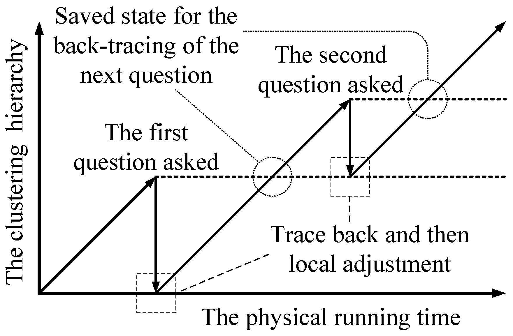
Our solution to the “how” problem is (1) first tracing back to a previous clustering state; (2) then doing local adjustment; and (3) finally resuming the building of the clustering hierarchy. It is shown in Figure 6 (assume that the human’s answer disagrees with the machine’s clustering results for the two questions). The depth of the back-tracing represents the trade-off between the time complexity and the accuracy. To limit the depth of the back-tracing, the machine only traces back to the hierarchy of the latest adjustment, as shown in Figure 6 (for the first question, the machine traces back to the initial state). After doing local adjustment, the machine resumes building the clustering hierarchy without question operations. The question operations are disabled until the machine goes back up the hierarchy that was present when it asked the question. Once the adjustment of the current question is finished, the state of the clustering is saved as the point to trace back to for the next question. Since each hierarchical state is calculated at most twice, this scheme at most doubles the time complexity.
Let us go over the machine’s process of dealing with the human’s answers. Suppose i and j are the most questionable pair of data points in the dirtiest cluster C: (1) if the human returns an answer that i and j are in the same cluster (agree with the machine), then everything is fine. i and j are removed for further questioning, and their distance is set to be 0; (2) if the human returns an answer that i and j are not in the same cluster (disagree with the machine), the machine traces back and then uses the local adjustment, which is referred to as a local splitting of C. In other words, C is divided into two clusters. The remaining data points in C choose to join i’s cluster or j’s cluster, according to the distance (join the nearest one). i and j are removed for the further questions, and their distance is set to be infinity. After this local adjustment, the machine resumes building the clustering hierarchy. The questions are disabled until the machine goes back to the point in the hierarchy at which it asked the question. In addition, note that the transitive relations of questions may bring the machine a derived answer in which two data points in different clusters should be in the same cluster. For this case, we refer to the local adjustment as a merge of the two clusters corresponding to those two data points. The distance between those two data points is set to be zero.
5. Algorithm Overview
5.1. Algorithm Design
The whole algorithm is presented in Algorithm 3, which is the detailed implementation of Algorithm 2. In Algorithm 3, line 5 corresponds to the “when” problem: the key insight is that questions are asked to limit the error propagations. Line 6 corresponds to the “which” problem: the key insight is that local structures of pairs of data points can be used to determine the most questionable pair of data points. Then, line 7 shows the transitive relations that can be used to derive more answers. If one of these answers disagrees with the current clustering result (i.e., the machine has made some errors), then adjustments are applied (lines 8 to 13), which correspond to the “how” problem. The key insight is that the back-tracing scheme can balance the time complexity and the adjustment accuracy. Line 14 shows that one question operation is used up. In the next subsection, further analysis shows that the time complexity of Algorithm 3 stays asymptotically the same with Algorithm 1, which is . We do not further discuss the stop criterion (line 3 in Algorithm 3). A simple stop criterion is used: the iteration stops, when the number of existing clusters reduces to a threshold. A better stop criterion is to be addressed in our future work.
| Algorithm 3: The Proposed Algorithm. |
| Data: Distances between pairs of data points; The number of available questions (i.e., Q). |
| Result: The clustering result. |
 |
5.2. Time Complexity Analysis
This section discusses the time complexity of Algorithm 3. First, we clarify the time complexity of Algorithm 1. In Algorithm 1, finding the closest two clusters at each clustering step takes , since there are at most pairs of clusters. Meanwhile, we have at most clustering steps (i.e., the number of iterations). Thus, the time complexity of Algorithm 1 is . However, this time complexity can be reduced, if each cluster keeps a sorted list (or heap) on its distances to all the other clusters: then, finding the closest two clusters at each clustering step is reduced to . Considering that maintaining the sorted list (or heap) needs an additional time complexity of , the time complexity of Algorithm 1 should be .
Then, let us focus on the time complexity of Algorithm 3. First, note that the additional time complexity is brought by lines 5 to 14. Then, to calculate the certainty, lines 5 and 6 take for each clustering step, since each cluster can maintain and update the certainties brought by pairs of data points. Exhaustive derivation of transitive relations in line 7 takes in total . As previously mentioned, the tracing-back scheme (lines 10 and 11) at most doubles the time complexity. The local adjustments take for each time, up to in total. Saving the current clustering state (line 13) takes for each time, also up to in total. Therefore, the overall time complexity is . Both k and Q are relatively small numbers, when compared to N. Note that k is used to define the neighborhood of one data point. Q is also limited, due to relatively costly human computations. Therefore, the time complexity of Algorithm 3 is , which is asymptotically the same as that of Algorithm 1. We assume that the human answers a question instantaneously. In other words, we consider that the computational time for the machine’s task is much longer than the question response time.
6. Experiments
This section conducts real data-driven experiments to evaluate the algorithm performance.
6.1. Data Set Descriptions
Our experiments are based on the Iris Flower Data Set [34,35,36] and the Labeled Faces in the Wild (LFW) Data Set [37]. The Iris Flower Data Set consists of 150 flowers from three species of Iris (Iris setosa, Iris virginica, and Iris versicolor). Flowers of the same species are supposed to be clustered together. It is easy for a trained human to judge whether two Iris flowers belong to the same species or not. For each flower (i.e., a data point), four features are collected: sepal length, sepal width, petal length, and petal width. For each feature, we re-scale its range into . Euclidean distances are calculated as the distances between pairs of Iris flowers. In this data set, four questions are available for the machine to ask. Then, the LFW Data Set is a database of face photographs designed for studying the problem of face clusterings. This data set contains face images collected from the web. Each face has been labeled with the name of the person pictured (detected by the Viola–Jones face detector). Our experiments use the first 100 images of two persons that have the largest and second-largest number of face images (200 images in total). Face images of the same person should be clustered together. It is easy for a trained human to judge whether two face images belong to the same person or not. For each image, 65 features are collected as [37]. For each feature, we also re-scale its range into . Euclidean distances are also used as the distances between pairs of face images. In the LFW Data Set, six questions are available for the machine to ask. In addition, is used to determine the neighborhood of a data point. Other datasets [38] are not used, since the hierarchical clustering may not perform well (HMC may be better applied to other clustering methodologies).
In practical usages, the value of k should be large enough to reveal the local structures of data points. k can also be determined by statistics on the distribution of neighborhood distances among data points. In the ideal scenario, an arbitrary data point and its k nearest neighbors are very likely to be in the same cluster. On the other hand, the value of Q can be arbitrary: a larger Q is expected to bring a more accurate clustering result but needs more human work. Q should scale up with respect to the squared number of data points, which shows the number of possible questions.
6.2. Algorithms for Comparison
Here, we denote the traditional agglomerative hierarchical clustering algorithm as TAHC, while the proposed algorithm is denoted as HMCAHC. Then, five different variations of the HMC strategies are used for comparison:
- Instead of picking the most questionable pair of data points, the machine asks questions based on a committee-based sampling strategy [39]. This algorithm is HMCAHC-which.
- Rather than asking questions upon certainty increases, the machine asks questions upon a certainty reduction (judged by a threshold of 0.1). This is because a large certainty reduction means that a newly merged cluster is not as pure as previous ones. The threshold is empirically determined. This algorithm is HMCAHC-when1.
- Instead of asking questions upon certainty gain, the machine asks questions upon a maximum entropy reduction [40] (judged by a threshold of 0.1). This algorithm is HMCAHC-when2.
- Rather than the back-tracing scheme, the machine uses local adjustments for the “how” problem. This algorithm is HMCAHC-how1.
- Instead of the back-tracing scheme, the machine uses global adjustments, in which the machine goes back to the initial state and redoes everything. This algorithm is as HMCAHC-how2. In general, HMCAHC-how2 should have a better result than HMCAHC, at the cost of a higher time complexity. While HMCAHC takes , HMCAHC-how2 takes .
K-Means is also used for comparison as a baseline algorithm. In addition, two constraint-based clustering algorithms are also used, i.e., PCMK-Means [22] and Active PCK-Means [23]. For these two algorithms, questions on random pairs of data points are asked before the algorithm execution, while the human’s answers serve as pre-given constraints. Our approach differs from these three classic algorithms for the “when” problem and the “how” problem. Moreover, the algorithm proposed by Roads et al. [5] is also compared (its set size is 10 for human comparisons).
In our real data-driven experiments, ground-truth clustering results are available. Therefore, the mutual information [41] is introduced to measure the similarity between the current clustering result and the ground-truth result. The mutual information falls into the interval of , where a higher value indicates a higher similarity (i.e., a better clustering quality). We are interested in the mutual information variance, when clusters are iteratively merged. Considering that our strategy favors asking questions in later steps, we focus on the mutual information variance among the last few clustering steps. The estimation accuracy of the machine’s certainty is also investigated. We will observe the difference between the machine’s certainty and the true minimum purity.
6.3. Evaluation Results (Iris Flower Data Set)
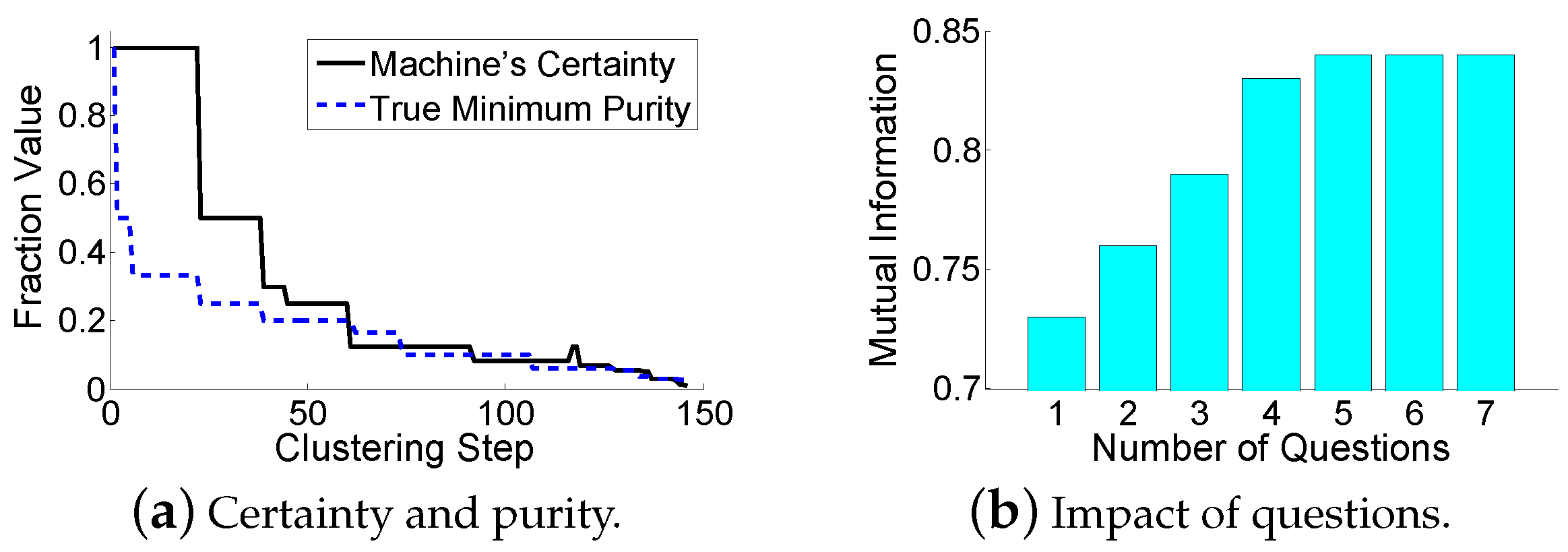
The evaluation results are shown in Table 1 and Table 2. All the algorithms stop iterations when there are three clusters remaining (the true number of clusters). In HMCAHC, the human agrees with the machine on the 1st and 2nd questions, but disagrees with the machine on the 3rd and 4th. For the “which” problem, it can be seen that asking the most questionable pair of data points in the dirtiest cluster (HMCAHC) is better than a committee-based sampling strategy (HMCAHC-which). This is because HMCAHC uses the uncertainty sampling with density weights. While the gap between the mutual information of the HMCAHC and the TAHC is about 0.1, the HMCAHC-which has almost no performance improvement. For the “when” problem, although asking questions upon a significant certainty reduction (HMCAHC-when1) and upon a maximum entropy reduction (HMCAHC-when2) provides a good foundation for the early clustering stage, they fail to reserve enough questions for the hard decisions. The error propagation is disastrous, and thus shuts down the performance of the HMCAHC-when1 and the HMCAHC-when2 in the later clustering stage. For the “how” problem, although the global adjustment (HMCAHC-how2) brings a slightly better result, this performance improvement is at the cost of a much higher time consumption. On the other hand, although the local adjustment (HMCAHC-how1) has less time consumption, it has a much worse result. Our back-tracing scheme obtains a result that is close to the global adjustment, at the cost of an acceptable time consumption. Meanwhile, both PCMK-Means and Active PCK-Means perform more poorly than HMCAMC. This is because they use the questions in the beginning as the clustering constraints. They fail to reserve the question operations for difficult decisions. For further analysis, Figure 7a shows that the machine’s certainty provides a good estimation of the true minimum purity during the clustering-building process. Figure 7b shows the relationship between the available number of question operations and the resulting mutual information of HMCAHC. It can be seen that a few questions can significantly improve the clustering results; however, too many question operations are unnecessary due to the marginal improvement. Compared to Roads’ approach, the proposed algorithm also has a performance improvement of 0.02 in terms of mutual information. Moreover, our approach requires less human operations than Roads’ approach. While our approach only asks the human to compare a few pairs of data points, Roads’ approach requires the human to compare a data point with a set of data points (our experiments set the set size to be 10).
6.4. Evaluation Results (LFW Data Set)
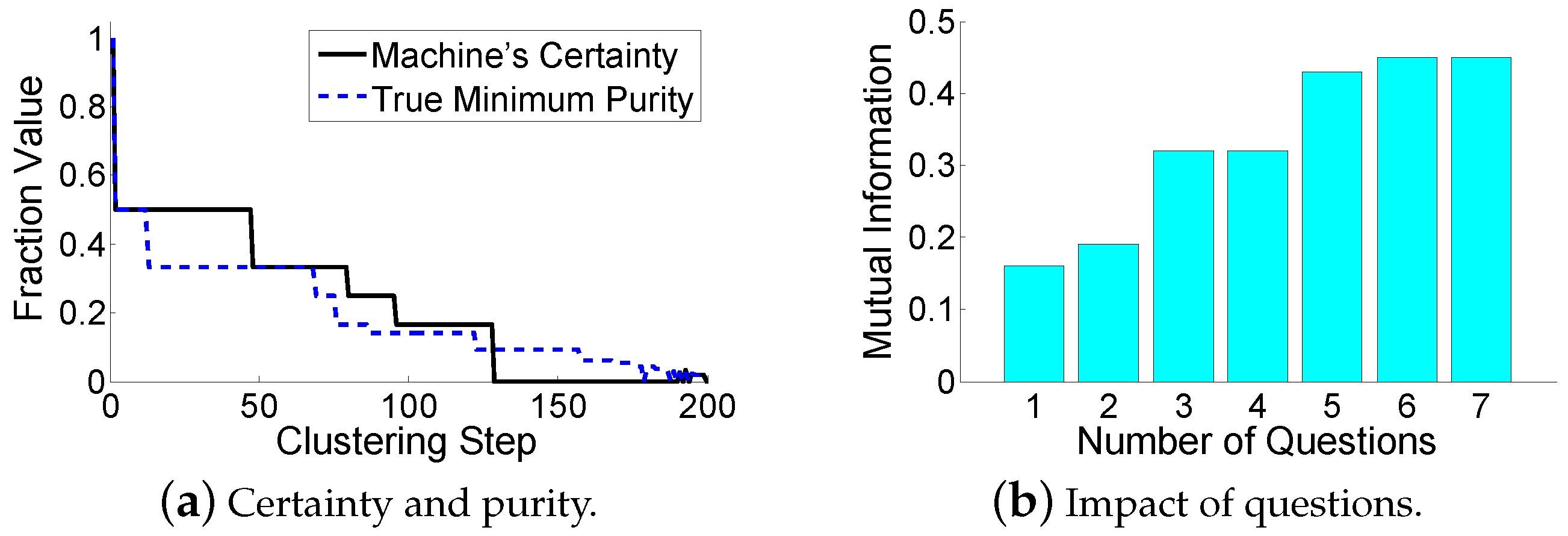
The evaluation results are shown in Table 3 and Table 4. All the algorithms stop iterations when there are two clusters remaining (the true number of clusters). It can be seen that all algorithms have relatively low resulting mutual information, since the face images have complex variations in pose and illumination. For TAHC, it even makes a seriously incorrect decision at the last step, leading to a performance degradation. For the “which” problem, HMCAHC is still better than HMCAHC-which, since a random question does not bring too much useful information for the machine. For the “when” problem, HMCAHC-when1 and HMCAHC-when2 fail to reserve enough questions for the hard decisions. The error propagation is disastrous, and thus shuts down the performance of the HMCAHC-when1 and the HMCAHC-when2 in the later clustering stage (especially for HMCAHC-when2 that makes an incorrect decision at the last step). For the “how” problem, the trade-off between the clustering accuracy and the time consumption is still observed by HMCAHC-how1 and HMCAHC-how2. Our back-tracing scheme balances this trade-off. Meanwhile, both PCMK-Means and Active PCK-Means perform more poorly than HMCAMC. This is because they fail to reserve the question operations (i.e., constraints) for really hard decisions. For further analysis, Figure 8a shows that the machine’s certainty has a good estimation of the true minimum purity during the clustering-building process. Figure 8b shows the relationship between the available number of question operations and the resulting mutual information of HMCAHC. Although a few questions can significantly improve the clustering results, too many question operations are unnecessary due to the marginal improvement.
7. Conclusions
Human–Machine Cooperations (HMCs) can balance the advantages and disadvantages of human computation (accurate but costly) and machine computation (cheap but inaccurate). We study HMCs in agglomerative hierarchical clustering problems with respect to image clustering applications. The machine can ask the human questions. We explore the machine’s strategy on handling the question operations, in terms of the “which” problem, the “when” problem, and the “how” problem. The “which” problem is solved by using the machine’s certainty with respect to data points. The “when” problem is solved by observing the oscillations of the minimum purity. The “how” problem is solved by balancing the local and global adjustments. As a result, an efficient HMC-based algorithm is proposed with five implementation variations. Experiments show the efficiency of the proposed algorithm.
Acknowledgments
This research was supported in part by NSF grants CNS 1449860, CNS 1461932, CNS 1460971, CNS 1439672, CNS 1301774, and ECCS 1231461.
Author Contributions
J.W. conceived and designed the experiments; H.Z. performed the experiments; H.Z. and J.W. analyzed the data; J.W. contributed reagents/materials/analysis tools; H.Z. wrote the paper. Authorship must be limited to those who have contributed substantially to the work reported.
Conflicts of Interest
The authors declare no conflict of interest.
References
- Hoc, J. From human–machine interaction to human–machine cooperation. Ergonomics 2000, 43, 833–843. [Google Scholar] [CrossRef] [PubMed]
- Swiechowski, M.; Merrick, K.; Mandziuk, J.; Abbass, H. Human–Machine Cooperation in General Game Playing. In Proceedings of the IARIA International Conference on Advances in Computer-Human Interactions (ACHI), Lisbon, Portugal, 22–27 February 2015.
- Shirahama, K.; Grzegorzek, M.; Indurkhya, B. Human–Machine Cooperation in Large-Scale Multimedia Retrieval: A Survey. J. Probl. Solving 2015, 3, 36–63. [Google Scholar] [CrossRef] [Green Version]
- Chauvin, C.; Hoc, J.M. Integration of Ergonomics in the Design of Human–Machine Systems. Des. Hum. Mach. Coop. Syst. 2014, 1, 43–86. [Google Scholar]
- Roads, B.D.; Mozer, M.C. Improving Human–Machine Cooperative Classification via Cognitive Theories of Similarity. Cognit. Sci. 2016, 1, 1–27. [Google Scholar] [CrossRef] [PubMed]
- Chang, J.C.; Kittur, A.; Hahn, N. Alloy: Clustering with Crowds and Computation. In Proceedings of the ACM Conference on Human Factors in Computing Systems (CHI), San Jose, CA, USA, 7–12 May 2016.
- Motoi, N.; Kubo, R. Human–Machine Cooperative Grasping/Manipulating System Using Force-Based Compliance Controller with Force Threshold. IEEJ J. Ind. Appl. 2016, 5, 39–46. [Google Scholar] [CrossRef]
- Biswas, A.; Jacobs, D. Active image clustering: Seeking constraints from humans to complement algorithms. In Proceedings of the IEEE Conference on Computer Vision and Pattern Recognition (CVPR), Columbus, OH, USA, 23–28 June 2014.
- Kumar, N.; Belhumeur, P.; Biswas, A.; Jacobs, D.; Kress, W.J.; Lopez, I.; Soares, J. Leafsnap: A computer vision system for automatic plant species identification. In Proceedings of the European Conference on Computer Vision (ECCV), Amsterdam, The Netherlands, 8–16 October 2012.
- Pangning, T.; Steinbach, M.; Kumar, V. Introduction to Data Mining; Pearson Education: Cranbury, NJ, USA, 2006. [Google Scholar]
- Balcan, M.F.; Gupta, P. Robust Hierarchical Clustering. In Proceedings of the International Conference on Learning Theory (COLT), Haifa, Israel, 27–29 June 2010.
- Ipeirotis, P.; Paritosh, P. Managing crowdsourced human computaiton. In Proceedings of the ACM International Conference on World Wide Web (WWW), Hyderabad, India, 28 March–1 April 2011.
- Parameswaran, A.; Sarma, A.; Garciamolina, H.; Polyzotis, N.; Widom, J. Human-Assisted Graph Search: It’s Okay to Ask Questions. In Proceedings of the International Conference on Very Large Data Bases (VLDB), Seattle, Washington, DC, USA, 29 August–3 September 2011.
- Park, T.; Saad, W. Learning with finite memory for machine type communication. In Proceedings of the Conference on Information Systems and Sciences (CISS), Princeton, NJ, USA, 16–18 March 2016.
- Melo, C.D.; Marsella, S.; Gratch, J. People do not feel guilty about exploiting machines. ACM Trans. Comput. Hum. Interact. 2016, 2, 1–17. [Google Scholar] [CrossRef]
- Brew, A.; Greene, D.; Cunningham, P. Using Crowdsourcing and Active Learning to Track Sentiment in Online Media. In Proceedings of the European Conference on Artificial Intelligence (ECAI), Lisbon, Portugal, 16–20 August 2010.
- Ramirez-Loaiza, M.E.; Culotta, A.; Bilgic, M. Anytime Active Learning. In Proceedings of the AAAI Conference on Artificial Intelligence (AAAI), Quebec City, QC, Canada, 27–31 July 2014.
- Wang, Z.; Ye, J. Querying discriminative and representative samples for batch mode active learning. ACM Trans. Knowl. Discov. Data 2015, 17. [Google Scholar] [CrossRef]
- Wei, K.; Iyer, R.; Bilmes, J. Submodularity in data subset selection and active learning. In Proceedings of the IMLS International Conference on Machine Learning (ICML), Lille, France, 6–11 July 2015.
- Loog, M.; Jensen, A.C. Constrained log-likelihood-based semi-supervised linear discriminant analysis. In Proceedings of the joint IAPR International Workshops on Structural and Syntactic Pattern Recognition (SSPR) and Statistical Techniques in Pattern Recognition (SPR), Montreal, QC, Canada, 11–14 July 2012.
- Loog, M.; Jensen, A.C. Semi-supervised nearest mean classification through a constrained log-likelihood. In Proceedings of the joint IAPR International Workshops on Structural and Syntactic Pattern Recognition (SSPR) and Statistical Techniques in Pattern Recognition (SPR), Grand Rapids, MI, USA, 19–23 July 2014.
- Basu, S.; Banerjee, A.; Mooney, R.J. Active Semi-Supervision for Pairwise Constrained Clustering. In Proceedings of the International Conference on Data Mining (SDM), Lake Buena Vista, FL, USA, 22–24 April 2004.
- Bilenko, M.; Basu, S.; Mooney, R.J. Integrating constraints and metric learning in semi-supervised clustering. In Proceedings of the IMLS International Conference on Machine Learning (ICML), Banff, AB, Canada, 4–8 July 2004.
- Ahn, K.; Cormode, G.; Guha, S.; McGregor, A.; Wirth, A. Correlation clustering in data streams. In Proceedings of the IMLS International Conference on Machine Learning (ICML), Lille, France, 6–11 July 2015.
- Ghoshdastidar, D.; Dukkipati, A. A provable generalized tensor spectral method for uniform hypergraph partitioning. In Proceedings of the IMLS International Conference on Machine Learning (ICML), Lille, France, 6–11 July 2015.
- Bahadori, M.T.; Kale, D.; Fan, Y.; Liu, Y. Functional subspace clustering with application to time series. In Proceedings of the IMLS International Conference on Machine Learning (ICML), Lille, France, 6–11 July 2015.
- Deng, K.; Bourke, C.; Scott, S.; Sunderman, J.; Zheng, Y. Bandit-based algorithms for budgeted learning. In Proceedings of the IEEE International Conference on Data Mining (ICDM), Omaha, NE, USA, 28–31 October 2007.
- Kukliansky, D.; Shamir, O. Attribute Efficient Linear Regression with Distribution-Dependent Sampling. In Proceedings of the IMLS International Conference on Machine Learning (ICML), Lille, France, 6–11 July 2015.
- Amin, K.; Kale, S.; Tesauro, G.; Turaga, D.S. Budgeted Prediction with Expert Advice. In Proceedings of the AAAI Conference on Artificial Intelligence (AAAI), Austin, TX, USA, 25–30 January 2015.
- Ali, A.; Kolter, J.Z.; Diamond, S.; Boyd, S. Disciplined convex stochastic programming: A new framework for stochastic optimization. In Proceedings of the Conference on Uncertainty in Artificial Intelligence (UAI), Amsterdam, The Netherlands, 13–15 July 2015.
- Böck, R.; Bonin, F.; Campbell, N.; Poppe, R. Multimodal Analyses Enabling Artificial Agents in Human–Machine Interaction; Springer: Berlin, Germany, 2015. [Google Scholar]
- Aggarwal, C.; Han, J.; Wang, J.; Yu, P. A framework for projected clustering of high dimensional data streams. In Proceedings of the International Conference on Very Large Data Bases (VLDB), Toronto, ON, Canada, 29 August–3 September 2004.
- Settles, B. Active Learning Literature Survey; Technical Report; University of Wisconsi: Madison, WI, USA, 2010. [Google Scholar]
- Bache, K.; Lichman, M. UCI Machine Learning Repository. 2013. Available online: http://archive.ics.uci.edu/ml (accessed on 15 December 2016).
- Downar, L.; Duivesteijn, W. Exceptionally Monotone Models–The Rank Correlation Model Class for Exceptional Model Mining. In Proceedings of the IEEE International Conference on Data Mining (ICDM), Altantic City, NJ, USA, 14–17 November 2015.
- Achtert, E.; Kriegel, H.P.; Schubert, E.; Zimek, A. Interactive data mining with 3D parallel coordinate trees. In Proceedings of the ACM Special Interest Group on Management of Data, New York, NY, USA, 22–27 June 2013.
- Kumar, N.; Berg, A.; Belhumeur, P.; Nayar, S. Attribute and Simile Classifiers for Face Verification. In Proceedings of the IEEE International Conference on Computer Vision (ICCV), Kyoto, Japan, 29 September–2 October 2009.
- Clustering Datasets by School of Computing; University of Eastern Finland, 2016. Available online: https://cs.joensuu.fi/sipu/datasets/ (accessed on 15 December 2016).
- Roy, N.; McCallum, A. Toward optimal active learning through monte carlo estimation of error reduction. In Proceedings of the IMLS International Conference on Machine Learning (ICML), Williamstown, MA, USA, 28 June–1 July 2001.
- McCallumzy, A.K.; Nigamy, K. Employing EM and pool-based active learning for text classification. In Proceedings of the IMLS International Conference on Machine Learning (ICML), Madison, WI, USA, 24–27 July 1998.
- Kraskov, A.; Stögbauer, H.; Andrzejak, R.; Grassberger, P. Hierarchical clustering using mutual information. Europhys. Lett. 2005, 2, 278. [Google Scholar] [CrossRef]
Figure 1.
Which question should the machine ask? Large circles are clusters.

Figure 2.
How does the machine adjust the current clustering result? Two strategies are shown. The large circles indicate clusters.
Figure 2.
How does the machine adjust the current clustering result? Two strategies are shown. The large circles indicate clusters.

Figure 3.
An example of the purity calculation. Small circles and squares are data points of different types. Data points of the same type should be clustered.
Figure 3.
An example of the purity calculation. Small circles and squares are data points of different types. Data points of the same type should be clustered.

Figure 4.
Counter-example.
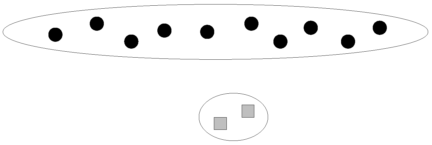
Figure 5.
The minimum purity and the “when” problem.

Figure 6.
The solution to the “how” problem.

Figure 7.
Evaluation results for the Iris Flower Data Set.

Figure 8.
Evaluation results for the LFW Data Set.


| Evaluation | The Mutual Information for Algorithms at Given Clustering Steps | ||||||||||
|---|---|---|---|---|---|---|---|---|---|---|---|
| Results | 1st | 50th | 100th | 120th | 130th | 140th | 142th | 144th | 145th | 146th | 147th |
| HMCAHC | 0.36 | 0.39 | 0.43 | 0.49 | 0.53 | 0.63 | 0.64 | 0.67 | 0.70 | 0.76 | 0.83 |
| HMCAHC-which | 0.36 | 0.39 | 0.43 | 0.50 | 0.53 | 0.63 | 0.60 | 0.64 | 0.66 | 0.69 | 0.76 |
| HMCAHC-when1 | 0.36 | 0.40 | 0.46 | 0.52 | 0.56 | 0.66 | 0.63 | 0.65 | 0.68 | 0.71 | 0.77 |
| HMCAHC-when2 | 0.36 | 0.41 | 0.45 | 0.50 | 0.55 | 0.65 | 0.61 | 0.63 | 0.66 | 0.68 | 0.75 |
| HMCAHC-how1 | 0.36 | 0.39 | 0.43 | 0.49 | 0.53 | 0.63 | 0.62 | 0.64 | 0.66 | 0.70 | 0.75 |
| HMCAHC-how2 | 0.36 | 0.39 | 0.43 | 0.49 | 0.53 | 0.63 | 0.66 | 0.69 | 0.73 | 0.80 | 0.84 |
| TAHC | 0.36 | 0.39 | 0.43 | 0.49 | 0.53 | 0.63 | 0.60 | 0.61 | 0.64 | 0.67 | 0.73 |
| K-Means | The mutual information of the final result is 0.75 | ||||||||||
| PCMK-Means | The mutual information of the final result is 0.76 | ||||||||||
| Active PCK-Means | The mutual information of the final result is 0.78 | ||||||||||
| Roads | The mutual information of the final result is 0.81 | ||||||||||
| Evaluation | Clustering Steps Where |
|---|---|
| Results | Questions Are Asked |
| HMCAHC | 117, 134, 142, 147 |
| HMCAHC-which | 117, 134, 142, 147 |
| HMCAHC-when1 | 23, 39, 45, 147 |
| HMCAHC-when2 | 30, 60, 90, 120 |
| HMCAHC-how1 | 117, 134, 142, 147 |
| HMCAHC-how2 | 117, 134, 142, 147 |
| Evaluation | The Resulting Mutual Information for Algorithms at Given Clustering Steps | ||||||||||
|---|---|---|---|---|---|---|---|---|---|---|---|
| Results | 1st | 50th | 100th | 150th | 170th | 180th | 190th | 192th | 194th | 196th | 198th |
| HMCAHC | 0.23 | 0.25 | 0.27 | 0.30 | 0.32 | 0.34 | 0.37 | 0.40 | 0.39 | 0.41 | 0.43 |
| HMCAHC-which | 0.23 | 0.25 | 0.26 | 0.30 | 0.31 | 0.34 | 0.43 | 0.37 | 0.34 | 0.34 | 0.37 |
| HMCAHC-when1 | 0.23 | 0.25 | 0.27 | 0.30 | 0.32 | 0.34 | 0.34 | 0.31 | 0.32 | 0.33 | 0.32 |
| HMCAHC-when2 | 0.23 | 0.25 | 0.27 | 0.30 | 0.31 | 0.34 | 0.34 | 0.31 | 0.34 | 0.33 | 0.16 |
| HMCAHC-how1 | 0.23 | 0.25 | 0.27 | 0.30 | 0.32 | 0.34 | 0.43 | 0.37 | 0.35 | 0.34 | 0.36 |
| HMCAHC-how2 | 0.23 | 0.25 | 0.27 | 0.30 | 0.32 | 0.34 | 0.37 | 0.40 | 0.41 | 0.42 | 0.45 |
| TAHC | 0.23 | 0.25 | 0.27 | 0.30 | 0.32 | 0.34 | 0.34 | 0.31 | 0.32 | 0.33 | 0.16 |
| K-Means | The mutual information of the final result is 0.30 | ||||||||||
| PCMK-Means | The mutual information of the final result is 0.32 | ||||||||||
| Active PCK-Means | The mutual information of the final result is 0.37 | ||||||||||
| Roads | The mutual information of the final result is 0.41 | ||||||||||
| Evaluation | Clustering Steps Where |
|---|---|
| Results | Questions Are Asked |
| HMCAHC | 177, 185, 186, 187, 188, 198 |
| HMCAHC-which | 177, 185, 186, 187, 188, 198 |
| HMCAHC-when1 | 12, 47, 64, 79, 86, 198 |
| HMCAHC-when2 | 28, 57, 85, 114, 142, 171 |
| HMCAHC-how1 | 177, 185, 186, 187, 188, 198 |
| HMCAHC-how2 | 177, 185, 186, 187, 188, 198 |
© 2016 by the authors; licensee MDPI, Basel, Switzerland. This article is an open access article distributed under the terms and conditions of the Creative Commons Attribution (CC-BY) license (http://creativecommons.org/licenses/by/4.0/).
Share and Cite
MDPI and ACS Style
Zheng, H.; Wu, J. Which, When, and How: Hierarchical Clustering with Human–Machine Cooperation. Algorithms 2016, 9, 88. https://doi.org/10.3390/a9040088
AMA Style
Zheng H, Wu J. Which, When, and How: Hierarchical Clustering with Human–Machine Cooperation. Algorithms. 2016; 9(4):88. https://doi.org/10.3390/a9040088
Chicago/Turabian StyleZheng, Huanyang, and Jie Wu. 2016. "Which, When, and How: Hierarchical Clustering with Human–Machine Cooperation" Algorithms 9, no. 4: 88. https://doi.org/10.3390/a9040088
Note that from the first issue of 2016, this journal uses article numbers instead of page numbers. See further details here.