Leaf Area Index, Biomass Carbon and Growth Rate of Radiata Pine Genetic Types and Relationships with LiDAR


Abstract
: Relationships between discrete-return light detection and ranging (LiDAR) data and radiata pine leaf area index (LAI), stem volume, above ground carbon, and carbon sequestration were developed using 10 plots with directly measured biomass and leaf area data, and 36 plots with modelled carbon data. The plots included a range of genetic types established on north- and south-facing aspects. Modelled carbon was highly correlated with directly measured crown, stem, and above ground biomass data, with r = 0.92, 0.97 and 0.98, respectively. LiDAR canopy percentile height (P30) and cover, based on all returns above 0.5 m, explained 81, 88, and 93% of the variation in directly measured crown, stem, and above ground live carbon and 75, 89 and 88% of the modelled carbon, respectively. LAI (all surfaces) ranged between 8.8–19.1 in the 10 plots measured at age 9 years. The difference in canopy percentile heights (P95–P30) and cover based on first returns explained 80% of the variation in total LAI. Periodic mean annual increments in stem volume, above ground live carbon, and total carbon between ages 9 and 13 years were significantly related to (P95–P30), with regression models explaining 56, 58, and 55%, respectively, of the variation in growth rate per plot. When plot aspect and genetic type were included with (P95–P30), the R2 of the regression models for stem volume, above ground live carbon, and total carbon increment increased to 90, 88, and 88%, respectively, which indicates that LiDAR regression equations for estimating stock changes can be substantially improved by incorporating supplementary site and crop data.1. Introduction
Radiata pine comprised approximately 90% of the 1.75 million hectares of planted forest estimated to occur in New Zealand in April 2009, a large proportion of which was established on grassland sites of moderate to high fertility predominantly between 1992 and 1998 [1]. Variation in stand growth rate reflects the level of genetic improvement and site factors. Volume growth rates of improved radiata pine seedlots typically average 20–30% higher than unimproved seedlots, and growth rates on fertile ex-pasture sites average approximately 20% higher than at sites without a pasture history [2].
A national inventory of carbon stocks in forest that existed prior to 1 January 1990 (Pre-1990 forest) and in new forest that was established on grassland after 31 December 1989 (Post-1989 forest) is providing data for New Zealand to meet its obligations under the Kyoto Protocol and the United Nations Framework Convention on Climate Change [3]. The Post-1989 inventory of Kyoto Compliant forest utilises ground plots established on a 4-km grid, supplemented with discrete-return small footprint airborne LiDAR (Light Detection And Ranging), utilizing a double sampling approach that aims to improve the precision of the national estimate of carbon stock change from 2008 to 2012. The majority of LiDAR-only plots are intended to be acquired along strip samples in 2012.
LiDAR has proven to be useful for assessing tree height, stand volume, and carbon stocks [4-8]. LiDAR regression equations typically explain from 70–90% of the variation in stand volume and carbon stocks. LiDAR is being used routinely in a number of countries [6] although technical issues related to data acquisition and analyses are still being addressed [9]. While field-based sampling remains an essential element of forest carbon inventory, the expected improvement in precision of New Zealand's national forest carbon stock estimates, when supplemented with LiDAR data, depends on the strength of LiDAR regression models.
LiDAR has also been used to estimate tree height growth, stem volume increment, and net primary production [10,11]. LiDAR sensors measure the vertical distribution of the pine canopy components, understorey tiers, and the ground, providing a three dimensional characterisation of stand structure [12]. Height growth can be estimated from repeated LiDAR flights, however a single LiDAR acquisition can provide estimates of leaf area index [13-17], and hence net primary production. Research is needed to determine the best method of estimating leaf area index using LiDAR.
In young stands, where live organic matter pools comprise a relatively large proportion of the total carbon stock, changes over time are due mostly to net dry matter production. Production, P can be predicted from leaf area index, solar radiation and radiation-use efficiency using the following relationship [18]:
Assuming that LiDAR point cloud metrics can provide robust estimates of the total LAI, we hypothesize, based on Equation 1, that information related to incident solar radiation level and radiation-use efficiency will improve the precision of stock change estimates. This hypothesis was tested in a pilot study at Puruki Forest by assessing the effects of site aspect and crop tree genetics on stem volume and carbon stock changes per plot in conjunction with using the best estimates of LAI we could derive using LiDAR.
2. Experimental Section
2.1. Puruki Forest Site and Trials
This study was undertaken at Puruki Forest [20], because the developmental stage and productivity of stands at this site are typical of many Kyoto forests in the North Island of New Zealand. Puruki is located at the southern end of the Paeroa Range mid-way between Rotorua and Taupo in the Central North Island of New Zealand. The topography is variable, ranging between easy rolling (slopes < 12°) to steep (30–38°), with elevations ranging from 530–650 m above sea level. The pumice soils originated from the Taupo eruption centre, which covers a large proportion of plantation forest estate in the Central North Island. Puruki was converted from improved grassland to radiata pine in 1973, and harvested and operationally replanted with radiata pine in 1997. In addition, three trials (FR443 series) were planted at Puruki in 1997 [21]. The trial plots were measured in 2006 and re-measured in 2010 using field-based methods and airborne LiDAR.
In 2006 the understorey vegetation at Puruki comprised grasses and bracken fern approximately 0.5–1 m in height and woody vegetation, including the invasive Buddleia davidii Franch. (buddleia), and the indigenous Coriaria arborea Lindsay (tutu), Aristotelia serrata J.R. Forst & G. Forst. W.R.B. Oliv. (wineberry), Melicytus ramiflores J.R. Forst & G. Forst (mahoe) and Coprosma species, approximately 2–6 m in height. The pine canopy was beginning to close in 2006, and by 2010 light-demanding species such as bracken fern, tutu and buddleia had been largely suppressed and the understorey was dominated by shade tolerant wineberry and mahoe trees approximately 8–12 m in height. Understorey development was most pronounced at micro-sites with shady aspects, where the pines typically had thin transparent crowns.
Three trials were established using seedlings and cuttings with different levels of genetic improvement, GF# [22], where increasing values of # generally indicate improved tree diameter growth rate and stem form (straightness). Genetic types in trials included:
GF7 cuttings (clonally propagated seedlings from GF7 parents);
GF2 seedlings (seed from an unimproved land-race [2]);
Puruki Control (PC) seedlings (from a GF7 stand that was heavily thinned to improve crown health, so GF rating is not known);
GF30 seedlings (seed from a defined set of control pollinated parents with improved growth and form);
High Density (HD) seedlings (seed from a defined set of control pollinated parents with improved growth, form and wood density).
Trial 1 is comprised of six 50 × 50 m plots installed in juxtaposition, with each plot covering a range of slopes and aspects. Each plot was block planted with an identical set of 400 genetically different cuttings (genetic type 1) at a nominal stocking of 1,600 stems/ha. All trees (excluding severely malformed stems) were pruned between April and June 2003 to a nominal prune height of 3.5 m, and thinned in May–June 2003 to approximately 850 trees/ha. Trees were pruned again in November 2004 to a nominal prune height of 6.5 m.
Trial 2 is comprised of ten 50 × 50 m plots installed either singly or in juxtaposition, with each plot covering a range of slopes and mixed aspects. Plots were planted with alternating rows of cuttings (9 rows of genetic type 1) and seedlings (3 rows each of genetic types 3 and 4), with 10 trees per row, giving an initial stocking of 600 stems/ha. Approximately 400 trees/ha were pruned between April and June 2003 to a nominal prune height of 3.5 m. The following year approximately 350 trees/ha were pruned in November 2004 to a nominal prune height of 6.5 m. No thinning occurred in these plots. The GF30 and Puruki Control trees were beginning to overtop and hence tending to suppress some of the GF7 trees by 2010.
Trial 5 is comprised of twenty plots, each entirely planted with a single genetic type (two plots of type 2, and six plots each of types 3, 4 and 5). Eighteen plots were installed on either high (North-facing) or low (South-facing) solar radiation aspects, at an initial stocking of 1000 stems/ha, using a randomised block design. Two plots of genetic type 2 were installed on low radiation (south) aspects, owing to a limited supply of GF2 seed. Plots were mostly 40 × 40 m square plots (a 30 × 30 m measurement area with two buffer rows), although some were quadrilateral in shape (same plot area) where the terrain dictated this. Approximately 400 trees/ha were pruned between April and June 2003 to a nominal prune height of 3.5 m, and 350 trees/ha pruned again in November 2004 to a nominal prune height of 6.5 m. No thinning occurred in these plots.
Plot corners were marked with pulp boards visible in stereo-photographs acquired in February 2001 by New Zealand Aerial Mapping Ltd using standard survey methods, and plot locations accurately digitised using an analytical plotter.
2.2. Plot Measurements
Tree measurements included stem diameter at breast height (DBH) of all crop trees and total height, green crown height, prune height, and needle retention (count of needle age classes present in the lower half of the nominally live crown) of approximately every third tree per plot in Trials 2 and 5, and one tree per row per plot in Trial 1. Understorey mean height and cover of vegetation growing below the crown of height trees were assessed. In Trial 5, the number of branch clusters (or whorls) within the live crown of height trees was counted in 2006 to aid with sample tree selection for biomass and leaf area measurement, as described in the following section. The 2006 and 2010 field data were entered into the New Zealand Forest Research Institute Ltd Permanent Sample Plot system (PSP), to ensure appropriate data checking and quality control.
2.3. Measured Biomass Carbon and Leaf Area Index
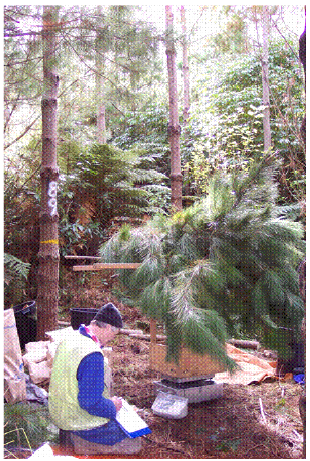
Leaf area was directly measured using biomass procedures, to avoid potential issues that have been identified when estimating LAI indirectly [23]. A total of 50 trees (five trees per plot) from 10 plots in Trial 5 were felled and weighed (Figure 1). Sample trees were selected on a stratified random basis, taking into account needle retention (NR) and whorl count/m of crown length, both of which determine crown transparency. This was achieved by ranking the trees in a plot according to their whorl count × NR score, and selecting every nth tree in this sequence as a biomass sample tree. Biomass trees were felled from 21 August–8 September 2006. Crowns were weighed fresh in the field by 2 m height zone, measured from the base of each tree. The specific leaf area of 50 fascicles per 2 m height zone was determined on an all surfaces basis following well established sampling and calculation methods [24]. Sample branches from each crown height zone were weighed fresh in the field, dried to constant weight at 65 degrees C, separated into needle and branch components, and weighed. Stem and crown component dry weights per ha and LAI by 2 m height zone were obtained by multiplying needle dry weight of each zone and tree by the corresponding specific leaf area, and expressing sample tree dry weights and leaf area on a per hectare basis (pre-biomass) using the basal area ratio method [25].
2.4. Modelled Carbon
Carbon stocks per plot were also estimated using a system referred to as the Forest Carbon Predictor (FCP) version 3. This carbon model is conditioned by plot summary attributes (BA, MTH, stocking) calculated from field measurements undertaken in 2006 and in 2010, which ensures that accurate estimates of stem volume and carbon are obtained per plot. Stem volume was estimated using a nationally applicable volume function incorporated within the 300 Index growth model [26]. The FCP couples the stem volume estimates from the 300 Index growth model [27] with either directly measured or modelled wood density estimates [28] and inputs these to a carbon partitioning model called C_Change [29]. Model outputs include stem volume, above ground live biomass (needles, branches, stems), below ground live biomass, dead wood, and litter pools.
Significant breast height density differences have been reported previously for seedlots in Trial 5, based on the mean density of the 6 outer growth rings of core samples from 20 trees per plot sampled at age 9 years [28]. Growth sheath density was estimated from the mean density of the outer 6 growth rings per plot using the wood density model. For plots in Trials 1 and 2 wood density was estimated from site data (soil C/N ratio and temperature) using the wood density model, so carbon stock estimates can be expected to be less accurate for these plots.
Natural and management related transfers of carbon from above- and below ground biomass pools to litter and dead wood pools were modelled for each plot, based on needle retention assessments, prune height data, and stocking changes following thinning operations [29].
2.5. LiDAR Data Acquisition
Airborne LiDAR data were acquired 1200 m over Puruki forest on 16 and 17 August 2006 and 13 March 2010 using an Optech ALTM 3100EA system by New Zealand Aerial Mapping (NZAM). The aircraft operated no more than 30 km from a GPS base-station forming part of the NZGD2000 geodetic network. The LiDAR point cloud data, which were supplied in LAS version 1.0 file format, met the specified vertical accuracy of 0.15 m and horizontal accuracy of 0.30 m. (Project 06.476 Data Supply Metadata Record). The data acquisition parameters are given in Table 1.
2.6. Summary of Stand Attributes
Table 2 provides a summary of stand attributes for the subset of 10 plots with biomass measurements in 2006, and for all 36 plots measured in 2006 and re-measured in 2010. Stand variables include mean top height (MTH) and basal area (BA) [30], prune height (Prune ht), needle retention (NR), stem volume inside bark/ha (Volib/ha), trees per ha (trees/ha), understorey height (Under Ht), and understorey cover (Under Cover). Carbon in above ground live biomass (AG Live C), below ground live biomass (BG Live C), coarse woody debris (Dead Wood C), branch and needle litter (Litter C), live plus dead biomass (Total C) in 2006 and 2010, and the periodic mean annual increment (PMAI) in stem volume and carbon stocks between ages 9 to 13 years were estimated using the carbon model. Crown carbon, stem carbon, and above ground live carbon and LAI by 2 m vertical layer were directly measured in 10 plots.
The 10 plots in Trial 5 with direct LAI measurements had a similar MTH but a higher basal area (24.1%) and stocking (17.5%) than plots in all three trials (Table 2). The total carbon stock at age 9 was comprised predominantly of above and below ground live tree carbon, followed by litter and a small amount of dead wood. The estimated total carbon stock change in four pools from stand age 9 to 13 years averaged 15 t/ha/year (Table 2), and was mostly due to changes in stem carbon.
The measured total LAI ranged between 8.8 and 19.1, with cumulative LAI profiles shown for each plot in Figure 2.
LAI vertical profiles were obtained for each plot by summing measurements by 2 m depth zone, starting at the top of the canopy down to specified heights above ground. For example, LAI_6 is the cumulative LAI from top of canopy to 6m above ground, and LAI_8 is the cumulative LAI from top of canopy to 8 m above ground. LAI data below 6 m above ground were within the partially unpruned part of the pine canopy where understorey shrubs often occurred.
2.7. Calculation of LiDAR Metrics
LiDAR metrics were calculated after normalizing the data by subtracting the bare ground elevation generated from the LiDAR bare-earth digital elevation model (DEM) at each XY coordinate of each return, from each LIDAR return elevation. Metrics were computed using the “Cloudmetrics” utility in FUSION [31], which requires decisions regarding the height thresholds to be applied for distinguishing ground returns from canopy returns, and whether to use first returns or all returns. The specified ground cut-off height is used to remove noise associated with the DEM, but can also be expected to remove returns from ground vegetation and debris on the forest floor. For all metrics, with the exception of cover, “Cloudmetrics” uses only those returns greater than a specified ground cut-off height.
Metrics calculated included canopy height percentiles of the point cloud above the specified ground height thresholds (5th, 10th, …, 95th) defined as P5, P10, …, P95 along with the mean height, several statistics describing the height distribution (standard deviation (Sd), coefficient of variation (Cv)), and canopy cover. LiDAR height percentiles were computed as follows: (1) using only the first returns within each pulse; or, (2) using all returns. Both first returns and all returns percentile metrics were computed with a 0.5 m ground height cut-off and 0.5 m cover height threshold. This cover height threshold includes returns from unpruned and partially pruned pines and from understorey vegetation greater than 0.5 m in height. Metrics were also calculated using 1 m/1 m, 1 m/3 m and 5 m/5 m as ground height/cover height cut-off thresholds. These thresholds can potentially affect the percentile heights, distribution statistics, and cover metrics, and were specified to determine the influence of returns from various understorey vegetation tiers and mean prune height on LiDAR relationships with the directly measured LAI.
Cover was computed by dividing returns above the cover height threshold by total number of returns (including those below the ground height cut-off) that were in the plot. Alternative estimates of canopy cover were computed as follows: (1) first returns from the canopy divided by first returns in the plot; and (2) all returns from the canopy divided by all returns in the plot. Use of all returns from canopy elements above the canopy height cut-off was expected to provide an improved characterisation of canopy cover [32]. Moreover, this study offered the opportunity to compare alternative LiDAR cover metrics with directly measured LAI.
2.8. Statistical Analysis
The GLM procedure of SAS (Windows Version 9.1, SAS Institute Inc., Cary, NC, USA) was used to develop regression equations between stand attributes of interest (Leaf area index, pine biomass, stem volume increment under bark, carbon sequestration) and radiata pine genetic type, aspect, and LiDAR metrics. Least squares means for genetic type and aspect were estimated across all 36 plots, after allowing for stocking differences between plots, to quantify genetic and micro-site related gains in volume increment and carbon sequestration rates at Puruki Forest.
LiDAR metrics were selected for inclusion in regression equations if they were biophysically meaningful, provided they were not strongly correlated with each other (r ≤ 0.5). LiDAR metrics selected to explain variation in LAI included cover because cover was expected to be low when there were gaps in the canopy and would be expected to increase with increasing canopy closure. However, by age 9 years, variation in LAI at Puruki was largely due to differences in crown transparency between plots, because the canopy had more-or-less closed. Percentile heights can be expected to be higher when crowns have dense compared with sparse foliage. Percentile heights would also be expected to increase with stand height. It was therefore considered necessary to include P95, a LiDAR metric highly correlated with canopy height, in regression equations with P30 and cover, to allow LAI to stabilise following canopy closure. Because P95 and P30 were moderately strongly correlated, the independent variable used in the regression model was (P95–P30). The influence of understorey vegetation on LiDAR metrics was tested empirically by examining the influence of variously calculated LiDAR height cut-off thresholds on LAI regression equations, and by including understorey height in place of cover in regression equations.
Measured and modelled biomass in crown, stem and stem plus crown components were separately regressed and compared using identical LiDAR metrics (percentile height and cover) as independent variables. Correlations between the measured and modelled biomass estimates were examined to provide confidence in the sequestration estimates obtained using the carbon model.
Finally, multiple regression analysis was used to test whether periodic mean annual increments in stem volume, above ground live carbon, and total carbon were related to LiDAR metrics identified as important for estimating LAI, and whether aspect and genetic type explained additional variation in growth, when fitted jointly with LAI-related LiDAR metrics.
3. Results
3.1. Effect of Genetic Type and Site on Stand Attributes
Substantial differences in stem volume growth rates were evident among genetic types (Table 3), with GF30 growing approximately 7%, 18%, and 26% faster than the HD, PC, and GF2 material, respectively, and 53% faster than the GF7 cuttings. A similar ranking was evident for carbon sequestration, although the gain depended on wood density which averaged 316 kg/m3 (GF30), 331 kg/m3(HD), 332 kg/m3 (GF2), and 332 kg/m3 (PC) in breast height outerwood density cores acquired at age 9 [28]. Hence, the GF30 seedlot sequestered carbon in above ground live biomass at approximately 0%, 10%, and 19% faster rate than the HD, PC, and GF2 material, respectively. Stem volume growth rate gains of GF30 relative to other genetic types were partially or, in the case of the HD seedlot, entirely nullified by wood density differences (Table 3).
Growth rate was substantially influenced by aspect, with volume increment and carbon sequestration rates approximately 30% higher at plots on sunny versus shady aspects (Table 3). No significant interaction was evident between genetic type and aspect.
3.2. Correlations among Stand Attributes and LiDAR Metrics
LiDAR metrics were in many cases highly correlated with each other. Correlations between canopy percentiles heights decreased the further these were apart, for example, for P95 the correlation was 0.9 with P70 and 0.5 with P30 in 2006. The canopy height standard deviation metric was strongly correlated with upper canopy height percentiles, but not significantly correlated with lower canopy height percentiles. The opposite was found for the coefficient of variation, which was strongly correlated with lower canopy height percentiles. Cover metrics were not significantly correlated with any of the other LiDAR metrics, apart from with each other and the lowest height percentile.
LiDAR metrics were also highly correlated with a subset of the stand attributes of interest. Mean top height was strongly correlated with upper height percentiles but not with height percentiles from P30 and below. LiDAR height metrics were also highly correlated with basal area, but more-so at lower height percentiles, peaking at around P30. Field measurements of understorey height were negatively correlated with mid-canopy height percentiles (indicating that plots with short pines had tall understorey vegetation), while the field estimates of understorey cover had moderately strong negative correlations with lower canopy height percentiles up to P60.
Correlations between LiDAR percentile height metrics and stem volume, above ground carbon, total carbon, litter carbon, carbon sequestration, and modelled LAI were all strong, with maximums at around P30. Dead wood, while only a small pool (Table 2), was weakly positively correlated with lower canopy height percentiles, possibly because dead wood arose as a result of light thinning of plots with high basal area.
Carbon sequestration and measured LAI were related to mid- and upper percentile heights, the coefficient of variation of heights (Cv), mean height, and to a lesser extent cover based on first returns. Intensity data were not used in the regression models given in this paper, but may be useful in stands with large accumulations of standing dead wood [33].
3.3. Effect of Ground and Canopy Threshold Heights, Return Number, and Plot Measurement Date on LiDAR Metrics
LiDAR metrics per plot based on first returns and all returns and using low (0.5 m/0.5 m) and high (5 m/5 m) ground height/cover height cut-off thresholds are shown for 2006 data in Table 4. Using a height cut-off of 5 m, which best matched the pruned pine canopy by excluding understorey shrubs and trees, minimum cover decreased markedly and minimum percentile heights increased for P30, while minimums and maximums for P95 were little affected, and variability in dispersion statistics decreased (Table 4). At low height cut-off thresholds, the P30 mean, minimum and maximum percentile heights for all returns were lower in the canopy than for first returns, and aligned more closely with prune height. In contrast, for P95 it made little difference to the percentile heights if first or all returns were used. Maximum cover (%) was 99% using first returns and 94% using all returns, so all returns may discriminate better between plots with high cover. Relative to 2006 data, percentage cover, percentile heights and Sd increased and Cv decreased in 2010 (Table 4).
3.4. Regressions between Measured LAI and LiDAR Metrics
Results of comparisons involving LiDAR metrics calculated using various height cut-off thresholds as predictors of cumulative LAI to 6 m above ground are shown in Table 5 for P30, although other percentile heights from P20–P80 gave similar results when fitted jointly with cover. Table 5 shows that lowering the base threshold height improved the model R2, due largely to an improvement in the P30 metrics relationship with leaf area. In the 5 m/5 m example, in which the cut-off height was approximately equal to the height down to which the bulk of the canopy LAI was measured, the cover metric and P30 metric were highly correlated with each other, with either metric significant when fitted on its own, although cover was superior to P30. While the LAI_6 regression model based on 5 m/5 m metrics explained 79% of the variation in LAI the model based on 0.5 m/0.5 m explained 88% of the variation. Metrics based on returns above 0.5 m height were therefore considered superior, and were used in the subsequent analyses.
The R2 values were higher when both percentile height and cover were based on all returns, for example, the model R2 increased from 88% to 91% using 0.5 m/0.5 m height cut-offs. Furthermore, field measured understorey height was highly significant in regressions of LAI down to 8 m height above ground, and partially substituted for the effect of cover, which was not considered desirable, given that understorey vegetation can vary markedly between stands and within stands over time.
The difference between upper and lower canopy percentile heights (P95–P30) calculated using all returns and cover based on first returns were significantly related to total LAI, with a model R2 of 80%. When substituted for LiDAR cover, understorey height was not statistically significant in these regressions.
3.5. Regression between Measured above Ground Live Biomass Carbon and LiDAR Metrics
Significant relationships were found between the measured and modelled crown, stem, and above ground (crown plus stem) carbon and P30 and LiDAR cover metrics based on all returns (Table 6). Measured volume and above ground live carbon averaged within 2% and 4%, respectively of modelled estimates, however the root mean square error (RMSE) for crown carbon and above ground live carbon increased by approximately 12–14%, respectively when modelled data were used. Of the various height percentiles tested, P30 was generally most strongly related to the directly measured stem volume and above ground biomass carbon. The regression model coefficients for P30 were all positive (Table 6), which indicates that percentile heights increased with increasing crown and stem biomass carbon. The P30 metric was statistically significant on its own, although the p-value of the model increased when fitted jointly with cover. The cover metric was important in regression equations for estimating stem and above ground carbon, but not crown carbon, although the sample size was small (10 plots).
3.6. Regression between Modelled above Ground Biomass Carbon and LiDAR Metrics
LiDAR regressions for estimating above ground live carbon stocks using P30 and cover, based on all 36 plots at Puruki, were more precise in 2006 than in 2010 (Table 7). Cover was not significant in 2010, possibly because canopy closure had occurred by age 13 years, and P30 on its own explained only 51% of the variation in above ground live carbon stocks.
Additional factors tested included genetic type, aspect and stocking-genetic type and stocking were highly significant, both in 2006 and 2010. The R2 of the base model in 2006 increased from 81%, using P30/cover, to 88% when genetic type was added and 91% when field measured stocking was added. Likewise, in 2010 the model R2 increased from 53%, using P30, to 91% when genetic type was added and 93% when field measured stocking was added. Similar results were obtained for stem total volume inside bark—the R2 of the model in 2006 increased from 81%, with P30/cover, to 87% with P30/cover/genetic type, and 90% with P30/cover/genetic type/ stocking. The corresponding model R2 values in 2010 were 49, 92 and 94%.
3.7. Regression between Periodic Mean Annual Increment in Stem Volume, above Ground Live Carbon, and Total Carbon Per Plot and LiDAR Metrics
Measured LAI in the 10 plots with biomass data explained 81% of the variation in above ground carbon sequestration and 79% of the variation in stem volume increment between age 9 and 13 years. The relationships with LAI were linear, as shown previously for radiata pine [19], unlike Equation 1 where P is linearly related to intercepted radiation. Moderately strong linear relationships were therefore expected between growth rate per plot and (P95–P30), with R2 values of 52 and 56% obtained using 2006 and 2010 LiDAR data, respectively (Table 8).
In addition, growth rate was significantly influenced by aspect, with R2 values increasing to approximately 74 and 76% using 2006 and 2010 LiDAR data (Table 8). When genetic type was added, (P95–P30) was not significant in 2006 (p-value averaged 0.33), but was significant in 2010 (p-value averaged 0.013). Adding stocking improved the R2 by an additional 3%, however the LiDAR metrics were not significant in 2006 (p-value averaged 0.083) but were significant in 2010 (p-value averaged 0.0058). While the effect of stocking was relatively small, the genetic types were ranked in accordance with growth expectations (Table 3) when stocking was included in the regression models.
P95 could substitute for stocking effects in the above models, which suggests that more refined national models could be developed in future, given that national data would be based on data across a wide range of stand ages and sites.
Linear regression models for predicting the PMAI in stem volume and above ground live carbon between ages 9 to 13 years are shown in Table 9, based on LiDAR data acquired at the end of the period (2010). The regression model coefficients for (P95–P30) were negative, which indicates that growth rates were higher in plots with dense crowns (i.e., with high LAI and therefore low penetration of LiDAR pulses) than in plots with sparse crowns (i.e., with low LAI and therefore high penetration of LiDAR pulses). Volume increment and carbon sequestration rates were above average in plots on high radiation (H) sites, below average on low radiation (L) sites, and intermediate in plots with mixed aspects (M), consistent with Equation 1. Furthermore, the most improved genetic types had significantly higher growth rates than unimproved types and material that originated from cuttings, which implies the existence of radiation-use efficiency differences among genetic types that were unable to be predicted using these LiDAR metrics for estimating LAI.
4. Discussion and Conclusions
Recent research has aimed to identify key LiDAR metrics that explain most of the variability in stand structural attribute across a range of forest types [34]. For example, tree average height was related to the standard deviation of all returns, however dominant height (Lorey's height) was most strongly correlated to the maximum return height [35]. Two LiDAR metrics (the 30th percentile canopy height and vegetation cover) explained approximately 80% of the variation in biomass carbon estimated to occur in radiata pine plantations covering a range of stand ages and stocking levels in New Zealand [36]. The same LiDAR metrics were important in the 9 year old plots in Puruki Forest, where direct biomass measurements showed that the carbon model provided accurate stock estimates, giving confidence in the carbon model estimates. Other researchers have suggested that species differences in crown geometry may underlie differences in model coefficients across sites [34].
We are not aware of LiDAR studies that have tested whether genetic improvement within a species influences LiDAR regression models. Most importantly, our analysis shows that inclusion of genetic type and aspect markedly improved the precision of LiDAR regression models based on (P95–P30), which provided the best estimate of LAI from LiDAR. LAI was measured directly at Puruki to avoid potential issues involved with deriving LAI indirectly [23]. We discuss our LiDAR derived estimates of LAI in detail below.
The results of our analysis were consistent with the productivity model (Equation 1) of Monteith [18], where LAI (represented in our analysis by (P95–P30)) incident solar radiation (represented by Aspect), and radiation-use efficiency (represented by Genetic type) determine growth, however relationships between PMAI Volib, PMAI AG live C and LAI were linear, as commonly reported for a range of tree species. Radiation-use efficiency has proven to be a robust approach for predicting growth in a wide range of situations [37]. It is known that genetic and environmental factors including temperature, elevated atmospheric carbon dioxide, site fertility, and water supply influence radiation-use efficiency to varying degrees [37-39]. These factors should ideally be further explored using national datasets, particularly for the pre-1990 planted forest estate which includes a wider range of genetic material and site types than the post-1989 planted forest estate.
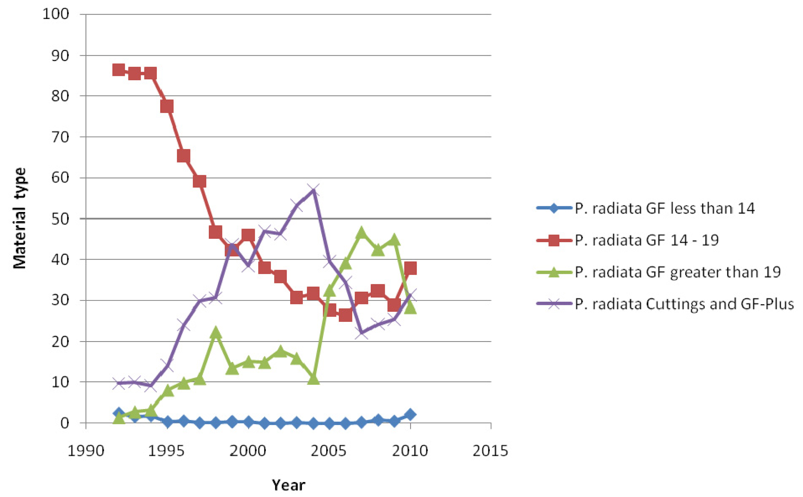
Our results are particularly relevant in the New Zealand context, because the quality of planting stock deployed in NZ's exotic forest estate has changed over time, and there has also been widespread adoption of clonally propagated cuttings (Figure 3). For example, a rapid decline in moderately improved GF 14–19 material occurred during the early to mid-1990's, followed by an increase in GF > 19 and GF-Plus seedling and cuttings. GF-Plus seedlings and cuttings were the favoured choice of highly improved stock prior to 2004, when large numbers of cuttings were being produced, due primarily to a lack of supply of GF > 19 seed. From 2004 it was evident that GF > 19 seedlings started to replace cuttings, because the latter were expensive to produce, although the trend has recently reversed (Figure 3). Changing the genetic type has unpredictable consequences on LiDAR regression models, and hence campaign-specific field-based measurements will be required for model calibration purposes.
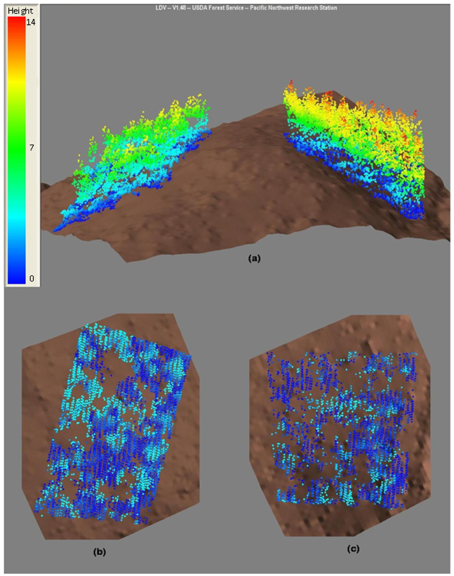
Cumulative LAI measurements from the top of the canopy down to 6 m above ground were strongly related to P30 and cover, although these plots were of similar mean top height. Analysis of LAI profiles showed that LiDAR relationships were strong at all levels in the canopy however the model R2 tended to decrease with depth in the canopy. This weak tendency presumably reflects the fact that near-ground returns were absent below some tree crowns, nevertheless, an appreciable number of pulses penetrated the canopy, even when the LAI was high. For example, the plot with an LAI of 19.1 has 28% (2,886/10,450) of all returns within 3 m of the ground surface (Figure 4), whereas the plot with an LAI of 8.8 has 52% (4,826/9,293). Unlike passive optical remote sensors, which are known to saturate at high LAI's [40], LiDAR appeared to discriminate between radiata pine plots that differed widely in LAI, presumably because it provides a three dimensional characterisation of the canopy, as noted previously [12]. The field procedures for directly measuring leaf area at Puruki were particularly rigorous, which may explain why strong relationships with LiDAR metrics were evident.
LiDAR metrics based on all returns generally gave stronger relationships with LAI vertical profiles than metrics based on first returns. Other researchers [32] have found that the canopy-to-total first returns ratio was better than the canopy-to-total returns ratio when estimating fractional cover from hemispherical photography, although the improvement in precision was relatively small. We found that cover was not significantly related to cumulative LAI down to 6 m above ground, unless it was fitted jointly with canopy percentile height metrics.
Percentile heights were lower in the canopy when the pines had thin transparent crowns with a low LAI. The influence of understorey on regressions based on P30 for estimating LAI was demonstrated by substituting the field measured understorey heights for LiDAR derived cover metrics in regressions where low canopy height thresholds were used. Returns from understorey vegetation can be expected to reduce the canopy height percentiles, especially when the overstorey pines have thin transparent crowns that allow greater penetration of LiDAR pulses to the understorey. Additional research may help resolve issues with understorey [41]. The use of (P95–P30) in regression models appeared to reduce the impact of understorey vegetation, possibly reducing bias expected to arise from this source. In young stands a low threshold height needs to be used, otherwise a considerable proportion of the pine leaf area will be missed, but this is generally not the case in older stands. Further research on the effect of threshold height is warranted, particularly in regard to estimating carbon sequestration in very young stands and mature stands with an appreciable understorey.
Crown mass of radiata pine plantations increases up to canopy closure and then decreases [42]. To distinguish LAI differences in stands that differ in height, due to site and stand age effects, an upper crown metric such as P95 may be required in conjunction with (P95–P30). For example, canopy percentile heights, percentile height differences, and cover were important for estimating LAI using the best subsets regression procedure [16]. We note that LiDAR estimates of height growth were sufficiently robust to enable monitoring of changes in height percentiles over intervals of 3 or more years, even in a relatively slow growing species such as red pine [10].
One source of uncertainty relates to temporal variation in stand health (i.e., needle retention). Needle retention influences leaf area, and may therefore be expected to influence LiDAR canopy height metrics, and warrants further research. Survey specific LiDAR regression equations avoid many possible issues, provided that flight specification related issues associated with LiDAR data acquisition parameters are adequately standardised when applying these regressions [9]. For forest inventory purposes, the time of year is critical when assessing the influence of LiDAR metrics on LAI and stand growth rate, as the LiDAR metrics are largely determined by leaf area and tree height, which depend on the stage of development of the canopy. Leaf area of radiata pine is at a minimum in winter, but increases rapidly in spring as new foliage expands. LiDAR acquisition would best be undertaken during summer months, when most leaf expansion for the year has been completed and prior to needle abscission commencing, during which time LAI is reasonably stable for several months [43]. Evidence of site and campaign specific effects on LiDAR regression relationships suggests that relationships are not invariant over space and time [44]. The stock change regressions we developed were based on LiDAR data acquired during a single campaign using metrics that reflect variation in LAI, thereby potentially providing a robust method of estimating volume increment and carbon sequestration.


| LiDAR parameter | Specified |
|---|---|
| Flying height | 1,200 m above ground |
| Scan angle | Clipped to 7 degrees either side of nadir |
| Pulse density | 8–10/m2 |
| Beam divergence | 0.3 mrad (1/e) |
| Maximum returns/pulse | 4 |
| Clipped swath width | 295 m |
| Swath-to-swath overlap | Approximately 30% |
| Pulse frequency | 71 kHz |
| 10 plots with measured C and LAI | 36 re-measured plots with modelled C | ||||||||
|---|---|---|---|---|---|---|---|---|---|
| Age 9 years | Age 9 years | Age 13 years | |||||||
| Variable | Mean | Min | Max | Mean | Min | Max | Mean | Min | Max |
| MTH (m) | 13.0 | 11.6 | 14.6 | 13.4 | 11.0 | 16.0 | 20.1 | 17.2 | 22.5 |
| BA (m2/ha) | 32.4 | 21.0 | 48.9 | 25.6 | 12.5 | 46.2 | 45.1 | 25.0 | 73.3 |
| LAI | 12.7 | 8.8 | 19.1 | - | - | - | - | - | - |
| Needle retention | 2.02 | 0.97 | 2.64 | 1.95 | 0.97 | 2.64 | 1.87 | 1.34 | 2.75 |
| Prune height (m) | 4.1 | 3.6 | 4.6 | 4.5 | 3.5 | 5.7 | 4.5 | 3.5 | 5.7 |
| Volib (m3/ha) | 158 | 96 | 260 | 126 | 61.6 | 253 | 315 | 173 | 538 |
| Trees/ha | 846 | 678 | 977 | 704 | 424 | 933 | 685 | 412 | 911 |
| Under Ht (m) | 1.8 | 1.1 | 3.0 | 1.6 | 0.9 | 3.0 | 3.4 | 0.9 | 8.6 |
| Under Cover (%) | 67 | 40 | 82 | 66 | 36 | 84 | 42 | 9 | 90 |
| AG Live C (t/ha) | 39.1 | 24.2 | 58.9 | 34.5 | 17.6 | 71.4 | 83.0 | 46.1 | 138.7 |
| BG Live C (t/ha) | - | - | - | 9.3 | 4.8 | 18.1 | 18.7 | 10.3 | 31.3 |
| Dead wood C (t/ha) | - | - | - | 1.3 | 0.1 | 4.7 | 1.3 | 0.04 | 3.8 |
| Litter C (t/ha) | - | - | - | 9.3 | 3.7 | 19.5 | 11.6 | 5.5 | 21.9 |
| Total C (t/ha) | - | - | - | 55.4 | 26.2 | 109.5 | 114.6 | 62.0 | 194.3 |
| PMAI Volib (m3/ha/yr) | 47.2 | 27.8 | 73.1 | ||||||
| PMAI AG Live C (t/ha/yr) | 12.1 | 7.2 | 18.1 | ||||||
| PMAI Total C (t/ha/yr) | - | - | - | - | - | - | 14.9 | 9.0 | 23.0 |
| Least squares means (and 95% Confidence Intervals) | ||||
|---|---|---|---|---|
| Volume PMAI (m3/ha/year) | AG Live C PMAI (t/ha/year) | Total C PMAI (t/ha/year) | ||
| Genetic type | GF30 | 58.3 (52.9–63.8) | 14.2 (12.8–15.7) | 17.6 (15.6–19.9) |
| GF7 cuttings | 37.8 (30.6–45.0) | 10.1 (8.2–12.1) | 12.2 (9.6–14.8) | |
| GF7 cuttings | 47.7 (39.4–56.0) | 12.2 (9.9–14.5) | 15.0 (12.0–18.0) | |
| GF30/PC mix | ||||
| HD | 53.8 (48.0–59.7) | 14.0 (12.4–15.6) | 17.5 (15.4–19.6) | |
| GF2 | 45.8 (35.9–55.8) | 11.9 (9.2–14.6) | 14.8 (11.2–18.4) | |
| PC | 49.1 (43.0–55.3) | 12.8 (11.1–14.4) | 16.0 (13.8–18.3) | |
| Aspect | North-sunny | 55.6 (50.6–60.7) | 14.4 (13.0–15.7) | 18.1 (16.2–19.9) |
| Mixed aspect | 48.3 (44.1–52.6) | 12.4 (11.3–13.6) | 15.3 (13.7–16.8) | |
| South-shady | 42.3 (39.3–45.3) | 10.8 (10.0–11.6) | 13.3 (12.2–14.3) | |
| Metric | All returns except cover in 2006 (5 m/5 m) | First returns in 2006 (0.5 m/0.5 m) | All returns in 2006 (0.5 m/0.5 m) | All returns in 2010 (0.5 m/0.5 m) | ||||||||
|---|---|---|---|---|---|---|---|---|---|---|---|---|
| Mean | Min. | Max. | Mean | Min. | Max. | Mean | Min. | Max. | Mean | Min. | Max. | |
| Cover (%) | 64 | 38 | 93 | 86 | 69 | 99 | 75 | 61 | 94 | 91 | 85 | 97 |
| P30 (m) | 7.0 | 6.1 | 8.1 | 5.3 | 2.9 | 8.2 | 4.2 | 2.2 | 7.3 | 9.7 | 5.9 | 13.4 |
| P50 (m) | 7.8 | 6.8 | 9.1 | 7.0 | 4.6 | 9.2 | 6.3 | 3.7 | 8.5 | 12.1 | 8.9 | 15.2 |
| P70 (m) | 8.8 | 7.5 | 10.3 | 8.3 | 6.4 | 10.4 | 7.9 | 5.9 | 9.8 | 14.0 | 11.2 | 16.8 |
| P95 (m) | 10.8 | 9.0 | 12.6 | 10.5 | 8.7 | 12.6 | 10.3 | 8.6 | 12.4 | 17.2 | 14.8 | 19.7 |
| Mean height (m) | 7.9 | 6.9 | 9.2 | 6.7 | 4.7 | 9.1 | 5.9 | 4.3 | 8.0 | 11.4 | 8.6 | 14.2 |
| Sd (m) | 1.6 | 1.1 | 1.9 | 2.6 | 2.0 | 3.5 | 3.0 | 2.4 | 3.6 | 4.2 | 3.2 | 5.5 |
| Cv (%) | 20 | 17 | 23 | 41 | 26 | 58 | 51 | 36 | 68 | 37 | 28 | 49 |
| Height cut-off thresholds | LAI depth zone | p-value | Model R2 (%) | |
|---|---|---|---|---|
| P30 | Cover (%) | |||
| 0.5 m/0.5 m | Log(LAI_6) | 0.0002 | 0.0368 | 88 |
| 1 m/1 m | Log(LAI_6) | 0.0006 | 0.0403 | 85 |
| 1 m/3 m | Log(LAI_6) | 0.0124 | 0.1317 | 80 |
| 5 m/5 m | Log(LAI_6) | 0.6031 | 0.0896 | 79 |
| Crown | Stem | Crown plus Stem | ||||||||
|---|---|---|---|---|---|---|---|---|---|---|
| R2 (%) | RMSE | p-value | R2 (%) | RMSE | p-value | R2 (%) | RMSE | p-value | ||
| Measured biomass | Regression | 81 | 1.69 | 0.0028 | 88 | 3.15 | 0.0005 | 93 | 3.40 | 0.0001 |
| Estimate (s.e.) | t-value | p-value | Estimate (s.e.) | t-value | p-value | Estimate (s.e.) | t-value | p-value | ||
| Intercept | −7.6 (6.8) | −1.1 | 0.300 | −38.4 (12.6) | −3.0 | 0.019 | −46.0 (13.6) | −3.4 | 0.012 | |
| P30 | 2.2 (0.40) | 5.5 | 0.001 | 5.4 (0.75) | 7.2 | 0.0002 | 7.6 (0.81) | 9.3 | <0.0001 | |
| Cover(%) | 0.10 (0.072) | 1.4 | 0.21 | 0.52 (0.13) | 3.9 | 0.006 | 0.62 (0.14) | 4.3 | 0.004 | |
| R2 (%) | RMSE | p-value | R2 (%) | RMSE | p-value | R2 (%) | RMSE | p-value | ||
| Modelled biomass | Regression | 75 | 1.89 | 0.0075 | 89 | 3.60 | 0.0005 | 88 | 5.00 | 0.0007 |
| Estimate (s.e.) | t-value | p-value | Estimate (s.e.) | t-value | p-value | Estimate (s.e.) | t-value | p-value | ||
| Intercept | −13.0 (7.6) | −1.7 | 0.13 | −47.5 (14.5) | −3.3 | 0.013 | −60.7 (20.1) | −3.0 | 0.019 | |
| P30 | 2.1 (0.45) | 4.6 | 0.002 | 6.3 (0.86) | 7.3 | 0.0002 | 8.4 (1.19) | 7.0 | 0.0002 | |
| Cover (%) | 0.15 (0.08) | 1.9 | 0.10 | 0.58 (0.15) | 3.8 | 0.007 | 0.74 (0.21) | 3.5 | 0.011 | |
| 2006 at age 9 years | 2010 at age 13 years | |||||
|---|---|---|---|---|---|---|
| R2 (%) | RMSE | p-value | R2 (%) | RMSE | p-value | |
| Model | 81 | 5.95 | < 0.0001 | 53 | 16.35 | < 0.0001 |
| Estimate (s.e.) | t-value | p-value | Estimate (s.e.) | t-value | p-value | |
| Intercept | −45.8(10.2) | −4.5 | 0.001 | −115.0 (94.3) | −1.22 | 0.23 |
| P30 | 7.52 (0.70) | 10.7 | < 0.0001 | 10.2 (1.73) | 5.90 | < 0.0001 |
| Cover (%) | 0.67 (0.13) | 5.2 | < 0.0001 | 1.09 (0.94) | 1.16 | 0.25 |
| Dependent Variable | Number of Independent Variables | Model | R2 (%) 2006 | R2 (%) 2010 |
|---|---|---|---|---|
| PMAI in Volume | 1 | P95–P30 | 53 | 56 |
| 2 | P95–P30, Aspect | 73 | 75 | |
| 3 | P95–P30, Aspect, Genetic type | 90 | ||
| 4 | P95–P30, Aspect, Genetic type, Stocking | 93 | ||
| PMAI in AG Live C | 1 | P95–P30 | 53 | 58 |
| 2 | P95–P30, Aspect | 75 | 77 | |
| 3 | P95–P30, Aspect, Genetic type | 88 | ||
| 4 | P95–P30, Aspect, Genetic type, Stocking | 91 | ||
| PMAI in Total C | 1 | P95–P30 | 50 | 55 |
| 2 | P95–P30, Aspect | 75 | 77 | |
| 3 | P95–P30, Aspect, Genetic type | 88 | ||
| 4 | P95–P30, Aspect, Genetic type, Stocking | 91 |
| PMAI Volib | PMAI AG live C | |||||
|---|---|---|---|---|---|---|
| R2 (%) | RMSE | p-value | R2 (%) | RMSE | p-value | |
| 93 | 3.79 | < 0.0001 | 91 | 1.06 | < 0.0001 | |
| Estimate (s.e.) | t-value | p-value | Estimate (s.e.) | t-value | p-value | |
| Intercept | 44.3 (9.62) | 4.61 | 0.0001 | 11.8 (2.70) | 4.37 | 0.0002 |
| P95–P30 | −3.005 (0.92) | −3.27 | 0.0030 | −0.755 (0.26) | −2.93 | 0.0069 |
| Radiation = H | 6.865 (2.19) | 3.13 | 0.0042 | 1.83 (0.62) | 2.97 | 0.0063 |
| = M | 0.0 | 0.0 | ||||
| = L | −1.990 (2.07) | −2.07 | 0.3455 | −0.62 (0.58) | −1.07 | 0.2949 |
| Genetic type = GF30 | 8.68 (2.31) | 3.76 | 0.0009 | 1.35 (0.65) | 2.09 | 0.0464 |
| = HD | 4.73 (2.25) | 2.10 | 0.0451 | 1.22 (0.63) | 1.93 | 0.0649 |
| = GF7 cuttings/PC/GF30 | 3.82 (4.06) | 0.942 | 0.3550 | 0.77 (1.14) | 0.674 | 0.5061 |
| = PC | 0 | 0 | ||||
| = GF2 | −3.70 (3.19) | −1.16 | 0.2559 | −0.97 (0.89) | −1.08 | 0.2887 |
| = GF7 cuttings | −11.19 (2.39) | −4.48 | 0.0001 | −2.60 (0.67) | −3.87 | 0.0007 |
| Stocking | 0.0345 (0.01) | 3.626 | 0.0012 | 0.008 (0.003) | 3.14 | 0.0045 |
Acknowledgments
We thank the Ministry for the Environment (MfE) for funding the measurement of permanent sample plots and biomass and leaf area measurements at Puruki. We would also like to thank field personnel who helped assess tree growth, health and leaf area at Puruki, in particular Doug Graham. Rod Brownlie provided accurate location data for the trial plots at Puruki. The LiDAR data and aerial photography over Puruki Forest were acquired by New Zealand Aerial Mapping. We also would like to thank John Novis, Ministry of Agriculture and Forestry, for providing information on the genetic quality of radiata pine from nursery surveys.
References
- A National Exotic Forest Description as at 1 April 2009; Ministry of Agriculture and Forestry: Wellington, New Zealand, 2010.
- Carson, S.D.; Garcia, O.; Hayes, J.D. Realized gain and prediction of yield with genetically improved Pinus radiata in New Zealand. For. Sci. 1999, 45, 186–200. [Google Scholar]
- Beets, P.N.; Brandon, A.; Fraser, B.V.; Goulding, C.J.; Lane, P.M.; Stephens, P.R. National Forest Inventories Report: New Zealand. In National Forest Inventories: Pathways for Common Reporting; Tomppo, E., Gschwantner, T., Lawrence, M., McRoberts, R.E., Eds.; Springer: Heidelberg, German, 2010; pp. 391–410. [Google Scholar]
- Næsset, E. Estimating timber volume of forest stands using airborne laser scanner data. Rem. Sens. Environ. 1997, 61, 246–253. [Google Scholar]
- Lefsky, M.A.; Cohen, W.B.; Harding, D.J.; Parker, G.G.; Acker, S.A.; Gower, S.T. Lidar remote sensing of above-ground biomass in three biomes. Glob. Ecol. Biogeogr. 2002, 11, 393–399. [Google Scholar]
- Næsset, E.; Gobakken, T.; Holmgren, J.; Hyyppä, H.; Hyyppä, J.; Maltamo, M.; Nilsson, M.; Olsson, H.; Persson, Å.; Söderman, U. Laser scanning of forest resources: The nordic experience. Scand. J. Forest. Res. 2004, 19, 482–499. [Google Scholar]
- Patenaude, G.; Milne, R.; Dawson, T.P. Synthesis of remote sensing approaches for forest carbon estimation: Reporting to the Kyoto Protocol. Environ. Sci. Pol. 2005, 8, 161–178. [Google Scholar]
- Reutebuch, S.E.; Andersen, H.E.; McGaughey, R.J. Light detection and ranging (LIDAR): An emerging tool for multiple resource inventory. J. Forest. 2005, 103, 286–292. [Google Scholar]
- Næsset, E. Effects of different sensors, flying altitudes, and pulse repetition frequencies on forest canopy metrics and biophysical stand properties derived from small-footprint airborne laser data. Rem. Sens. Environ. 2009, 113, 148–159. [Google Scholar]
- Hopkinson, C.; Chasmer, L.; Hall, R.J. The uncertainty in conifer plantation growth prediction from multi-temporal lidar datasets. Rem. Sens. Environ. 2008, 112, 1168–1180. [Google Scholar]
- Lefsky, M.A.; Turner, D.P.; Guzy, M.; Cohen, W.B. Combining LIDAR estimates of aboveground biomass and Landsat estimates of stand age for spatially extensive validation of modeled forest productivity. Rem. Sens. Environ. 2005, 95, 549–558. [Google Scholar]
- Lefsky, M.A.; Cohen, W.B.; Acker, S.A.; Parker, G.G.; Spies, T.A.; Harding, D. Lidar remote sensing of the canopy structure and biophysical properties of Douglas-fir western hemlock forests. Rem. Sens. Environ. 1999, 70, 339–361. [Google Scholar]
- Riaño, D.; Valladares, F.; Condés, S.; Chuvieco, E. Estimation of leaf area index and covered ground from airborne laser scanner (Lidar) in two contrasting forests. Agr. Forest. Meteorol. 2004, 124, 269–275. [Google Scholar]
- Farid, A.; Goodrich, D.C.; Bryant, R.; Sorooshian, S. Using airborne lidar to predict Leaf Area Index in cottonwood trees and refine riparian water-use estimates. J. Arid Environ. 2008, 72, 1–15. [Google Scholar]
- Hagiwara, A.; Imanishi, J.; Hashimoto, H.; Morimoto, Y. Estimating leaf area index in mixed forest using an airborne laser scanner. Int. Arch. Photogramm. Remote Sens. Spat. Inf. Sci. 2007, 36, 298–300. [Google Scholar]
- Jensen, J.L.R.; Humes, K.S.; Vierling, L.A.; Hudak, A.T. Discrete return lidar-based prediction of leaf area index in two conifer forests. Remote Sens. Environ. 2008, 112, 3947–3957. [Google Scholar]
- Solberg, S.; Brunner, A.; Hanssen, K.H.; Lange, H.; Næsset, E.; Rautiainen, M.; Stenberg, P. Mapping LAI in a Norway spruce forest using airborne laser scanning. Rem. Sens. Environ. 2009, 113, 2317–2327. [Google Scholar]
- Monteith, J.L.; Moss, C.J. Climate and the efficiency of crop production in Britain. Philos. Trans. R. Soc. London B 1977, 281, 277–294. [Google Scholar]
- Beets, P.N.; Whitehead, D. Carbon partitioning in Pinus radiata stands in relation to foliage nitrogen status. Tree Phys. 1996, 16, 131–138. [Google Scholar]
- Beets, P.N.; Brownlie, R.K. Puruki experimental catchment: Site, climate, forest management, and research. New Zeal. J. Forest. Sci. 1987, 17, 137–160. [Google Scholar]
- Beets, P.N.; Oliver, G.R.; Kimberley, M.O.; Pearce, S.H.; Rodgers, B. Genetic and soil factors associated with variation in visual magnesium deficiency symptoms in Pinus radiata. Forest. Ecol. Manag. 2004, 189, 263–279. [Google Scholar]
- Vincent, T.G. Certification System for Forest Tree Seed and Planting Stock; New Zealand Forest Research Institute Ltd: Rotorua, New Zealand, 1987. [Google Scholar]
- Breda, N.J.J. Ground-based measurements of leaf area index: A review of methods, instruments and current controversies. J. Exp. Bot. 2003, 54, 2403–2417. [Google Scholar]
- Beets, P.N.; Lane, P.M. Specific leaf area of Pinus radiata as influenced by stand age, leaf age, and thinning. New Zeal. J. Forest. Sci. 1987, 17, 283–291. [Google Scholar]
- Madgwick, H.A.I. Estimating the above-ground weight of forest plots using the basal area ratio method. New Zeal. J. Forest. Sci. 1981, 11, 278–286. [Google Scholar]
- Kimberley, M.O.; Beets, P.N. National volume function for estimating total stem volume of Pinus radiata stands in New Zealand. New Zeal. J. Forest. Sci. 2007, 37, 355–371. [Google Scholar]
- Kimberley, M.; West, G.; Dean, M.; Knowles, L. The 300 index—A volume productivity index for radiata pine. New. Zeal. J. Forest. 2005, 50, 13–18. [Google Scholar]
- Beets, P.N.; Kimberley, M.O.; McKinley, R.B. Predicting wood density of Pinus radiata annual growth increments. New Zeal. J. Forest. Sci. 2007, 37, 241–266. [Google Scholar]
- Beets, P.N.; Robertson, K.A.; Ford-Robertson, J.B.; Gordon, J.; Maclaren, J.P. Description and validation of C_Change: A model for simulating carbon content in managed Pinus radiata stands. New Zeal. J. Forest. Sci. 1999, 29, 409–427. [Google Scholar]
- Dunlop, J. Permanent Sample Plot System User Manual; New Zealand Forest Research Institute: Rotorua, New Zealand, 1995. [Google Scholar]
- McGaughey, R.J. FUSION/LDV: Software for LIDAR Data Analysis and Visualization. FUSION Version 2.70; USDA, Forest Service, Pacific Northwest Research Station: Seattle, WA, USA, 2009. [Google Scholar]
- Hopkinson, C.; Chasmer, L. Testing LiDAR models of fractional cover across multiple forest ecozones. Rem. Sens. Environ. 2009, 113, 275–288. [Google Scholar]
- Kim, Y.; Yang, Z.; Cohen, W.B.; Pflugmacher, D.; Lauver, C.L.; Vankat, J.L. Distinguishing between live and dead standing tree biomass on the North Rim of Grand Canyon National Park, USA using small-footprint lidar data. Rem. Sens. Environ. 2009, 113, 2499–2510. [Google Scholar]
- Li, Y.Z.; Andersen, H.-E.; McGaughey, R. A comparison of statistical methods for estimating forest biomass from light detection and ranging data. West. J. Appl. Forest. 2008, 23, 223–231. [Google Scholar]
- Hopkinson, C.; Chasmer, L.; Lim, K.; Treitz, P.; Creed, I. Towards a universal LIDAR canopy height indicator. Can. J. Rem. Sens. 2006, 32, 139–152. [Google Scholar]
- Stephens, P.; Watt, P.; Loubser, D.; Haywood, A.; Kimberley, M. Estimation of carbon stocks in New Zealand planted forests using airborne scanning LiDAR. Int. Arch. Photogram. Rem. Sens. 2007, 36, 389–394. [Google Scholar]
- Bartelink, H.H.; Kramer, K.; Mohren, G.M.J. Applicability of the radiation-use efficiency concept for simulating growth of forest stands. Agr. Forest. Meteorol. 1997, 88, 169–179. [Google Scholar]
- McCrady, R.L.; Jokela, E.J. Canopy dynamics, light interception, and radiation use efficiency of selected loblolly pine families. For. Sci. 1998, 44, 64–72. [Google Scholar]
- DeLucia, E.H.; George, K.; Hamilton, J.G. Radiation-use efficiency of a forest exposed to elevated concentrations of atmospheric carbon dioxide. Tree Phys. 2002, 22, 1003–1010. [Google Scholar]
- Sampson, D.A.; Allen, H.L. Direct and indirect estimates of leaf area index (LAI) for lodgepole and loblolly pine stands. Trees Struct. Funct. 1995, 9, 119–122. [Google Scholar]
- Maltamo, M.; Packalén, P.; Yu, X.; Eerikäinen, K.; Hyyppä, J.; Pitkänen, J. Identifying and quantifying structural characteristics of heterogeneous boreal forests using laser scanner data. Forest. Ecol. Manag. 2005, 216, 41–50. [Google Scholar]
- Madgwick, H.A.I.; Jackson, D.S.; Knight, P.J. Above-ground dry matter, energy, and nutrient contents of trees in an age series of Pinus radiata plantations. New Zeal. J. Forest. Sci. 1977, 7, 445–468. [Google Scholar]
- Madgwick, H.A.I. Seasonal changes in the biomass of a young Pinus radiata stand. New Zeal. J. Forest. Sci. 1983, 13, 25–36. [Google Scholar]
- Rombouts, J.; Ferguson, I.S.; Leech, J.W. Campaign and site effects in LiDAR prediction models for site-quality assessment of radiata pine plantations in South Australia. Int. J. Rem. Sens. 2010, 31, 1155–1173. [Google Scholar]
© 2011 by the authors; licensee MDPI, Basel, Switzerland. This article is an open access article distributed under the terms and conditions of the Creative Commons Attribution license (http://creativecommons.org/licenses/by/3.0/).
Share and Cite
Beets, P.N.; Reutebuch, S.; Kimberley, M.O.; Oliver, G.R.; Pearce, S.H.; McGaughey, R.J. Leaf Area Index, Biomass Carbon and Growth Rate of Radiata Pine Genetic Types and Relationships with LiDAR. Forests 2011, 2, 637-659. https://doi.org/10.3390/f2030637
Beets PN, Reutebuch S, Kimberley MO, Oliver GR, Pearce SH, McGaughey RJ. Leaf Area Index, Biomass Carbon and Growth Rate of Radiata Pine Genetic Types and Relationships with LiDAR. Forests. 2011; 2(3):637-659. https://doi.org/10.3390/f2030637
Chicago/Turabian StyleBeets, Peter N., Stephen Reutebuch, Mark O. Kimberley, Graeme R. Oliver, Stephen H. Pearce, and Robert J. McGaughey. 2011. "Leaf Area Index, Biomass Carbon and Growth Rate of Radiata Pine Genetic Types and Relationships with LiDAR" Forests 2, no. 3: 637-659. https://doi.org/10.3390/f2030637