A Flexible Hybrid Model of Life Cycle Carbon Balance for Loblolly Pine (Pinus taeda L.) Management Systems


Abstract
: In this study we analyzed the effects of silvicultural treatments on carbon (C) budgets in Pinus taeda L. (loblolly pine) plantations in the southeastern United States. We developed a hybrid model that integrated a widely used growth and yield model for loblolly pine with published allometric and biometric equations to simulate in situ C pools. The model used current values of forest product conversion efficiencies and forest product decay rates to calculate ex situ C pools. Using the model to evaluate the effects of silvicultural management systems on C sequestration over a 200 year simulation period, we concluded that site productivity (site quality), which can be altered by silviculture and genetic improvement, was the major factor controlling stand C density. On low productivity sites, average net C stocks were about 35% lower than in stands with the default average site quality; in contrast, on high quality sites, C stocks were about 38% greater than average productivity stands. If woody products were incorporated into the accounting, thinning was C positive because of the larger positive effects on ex situ C storage, rather than smaller reductions on in situ C storage. The use of biological rotation age (18 years) was not suitable for C sequestration, and extended rotation ages were found to increase stand C stock density. Stands with an 18-year-rotation length had 7% lower net C density than stands with a 22-year-rotation length; stands with a 35-year-rotation length had only 4% more C than stands harvested at age 22 years. The C sequestered in woody products was an important pool of C storage, accounting for ∼34% of the average net C stock. Changes in decomposition rate, associated with possible environmental changes resulting from global climate change, affected C storage capacity of the forest. When decay rate was reduced to 10% or increased to 20%, the C stock in the dead pool (forest floor and coarse woody debris) was reduced about 11.8 MgC·ha−1 or increased about 13.3 MgC·ha−1, respectively, compared to the average decay rate of 15%. The C emissions due to silvicultural and harvest activities were small (∼1.6% of the gross C stock) compared to the magnitude of total stand C stock. The C model, based on empirical and biological relationships, appears appropriate for use in regional C stock assessments for loblolly pine plantation ecosystems in the southern U.S.1. Introduction
Carbon dioxide (CO2) emissions from fossil fuels have increased on average at a rate of 1.9% per year over the last decades [1], with atmospheric CO2 concentration rising at approximately 1.4 parts per million by volume per year [2]. As Sundquist et al. [3] pointed-out, mitigation of atmospheric CO2 requires an approach that combines reductions in CO2 emissions with increasing CO2 storage. One of the most effective mechanisms for offsetting carbon (C) emissions is the fixation of atmospheric CO2 into plant tissues [3,4]. In the United States (U.S.), forests represent over 90% of the terrestrial C sink, equivalent to 12 to 16% of the U.S. greenhouse gas (GHG) emissions [2], and southern pines represent around 36% of the terrestrial C stock in the conterminous U.S. [5]. The applications of sustainable forest management systems can increase C sequestration potential of managed forests [6]. For example, forests in the southeast and south-central U.S. could potentially capture CO2 equivalent to about 23% of GHG emissions of that region [7].
Managed southern pine forests have played a large role in C sequestration in the U.S. [8]. The land area of southern pine plantations has increased steadily over the past half century [6], with plantations today occupying more than 13 million ha [9]. Intensive management of southern pine plantations, using competition control, fertilization, and superior genotypes, can now increase productivity four-fold, compared to mid-1950s plantations [9]. Rotation length is known to affect C stored in forest stands [10,11] and the use of extended rotations has been proposed as an effective way to increase C sequestration for different forest types such as scots pine (Pinus sylvestris L.) [12], Douglas-fir (Pseudotsuga menziesi (Mirb.) Franco) [13] or slash pine (Pinus elliottii Engelm. var. elliottii) [14].
In managed forests, C stocks can be divided into two major pools: in situ C in standing biomass (above and below ground) and soil organic matter, and ex situ C sequestered in products created from harvested wood [15]. Sustainable forest management has the potential to greatly influence both in situ and ex situ C pools [6].
In this study, we assessed the effects of silvicultural treatments on forest C stocks per unit area in Pinus taeda L. (loblolly pine) plantations established in the southeastern U.S. Coastal Plain and Piedmont physiographic regions. Following the approach of Gonzalez-Benecke et al. [14], we developed a hybrid model that accounted for both in situ and ex situ C stocks. In situ C pool dynamics were determined using growth and yield models for loblolly pine [16,17], combined with allometric and biometric equations; ex situ C pool dynamics were determined using current values of industrial conversion efficiencies and product-specific decay rates [14]. The model, which also accounted for C costs of silvicultural operations, did not include changes in soil C. We used the model to investigate net C balance, expecting that: (i) extended rotation lengths would increase time-averaged C stocks; (ii) regimes that incorporated longer rotations and thinning would maximize C accumulation in ex situ C pools; (iii) increasing stand productivity through intensive silviculture would increase net C storage; and (iv) under similar site and silvicultural treatments, loblolly pine would accumulate more C than slash pine plantations.
2. Materials and Methods
2.1. Models
Allometric and biometric equations were combined with growth and yield models to estimate C stocks and dynamics for loblolly pine plantations in the southeast U.S. We used published loblolly pine growth and yield equations that could be broadly applied to Lower Coastal Plain, Upper Coastal Plain and Piedmont regions [16-18]. These equations predicted stand growth in basal area (BA, m2·ha−1), dominant height (Hd, m), number of surviving trees per hectare (Nha, trees·ha−1), quadratic mean diameter (QMD, the diameter of the trees of mean BA, cm) and total stem volume (V, m3·ha−1), using as inputs number of trees planted per hectare (Nha), site index (SI, the height (m) reached by the stand's dominant trees at a reference age of 25 years), type of site preparation (no soil preparation or bedding), weed control treatment (age and method of application, broadcast or banded), fertilization treatment (age and amount of N and P applied), and thinning timing and intensity (as a removal percentage from the surviving trees before thinning).
At each age, allometric equations (Table 1) [19-21] were used to estimate coarse root, stem, crown and total aboveground stand biomass from QMD and Nha simulated by the growth and yield model. Biomass estimations were corrected using log-bias correction following back-transformations [22]. Fine root biomass was estimated from fine root/needle mass ratios reported for stands younger than 5 years [23], and for stands 5 years and older [21]. Loblolly pine projected leaf area index (LAI, the ratio of leaf surface area supported by a plant to its corresponding horizontal projection on the ground, m2·m−2) and litterfall (BL; Mg·ha−1·year−1) were estimated from the model reported by Gonzalez-Benecke et al. [24]. Forest floor biomass accumulation (BF; Mg·ha−1) was determined as in Gonzalez-Benecke et al. [24] as the sum of yearly litterfall inputs corrected for decay loss using an equation to estimate decay rate of the forest floor [25]. This equation used site coordinates (latitude and longitude, in decimal units) as inputs to estimate decay rate and was in good agreement with decay rates reported for southern pines in the southeastern U.S. [26-28]. Understory biomass accumulation (BU; Mg·ha−1) was estimated from published equations [14] that used a 17-year chronosequence of understory and litterfall biomass [29].
Standing dead trees, estimated from mortality equations [19], were incorporated into the dead component of total biomass. A large fraction of the stand mortality occurred in diameter classes below the median, due to the effects of resource competition of suppressed and weakened trees [4,30]. Using diameter distribution models reported for unthinned and thinned plantations [16], the diameters at the 25th percentile (cm) were determined for each age. This diameter class was assumed to better represent the observed diameter class of dying trees [30]. Biomass of dying trees was computed in the same way as standing biomass, but diameters at the 25th percentile from the previous year were used instead of QMD to estimate individual tree biomass.
At the time of thinning, reductions in loblolly pine LAI were set to be proportional to reductions in BA due to thinning and, therefore, litterfall, forest floor and understory biomass were affected due to their LAI-dependence [24]. At thinning and final harvest (clear-cut), logging slash (root and crown biomass plus stem residues) from harvested tress were also included into flux calculations and incorporated into the dead biomass pool. Stem residues were obtained by assuming a harvest efficiency of 88% of V [31-34]. It was assumed that C storage in soil was not affected by forest management in southern pines plantations [7,35-38], therefore the model did not include changes in soil C. Carbon mass (MgC·ha−1) was calculated by using an average C content of 50% for loblolly pine and understory biomass components [6,39,40].
2.2. Model Validation
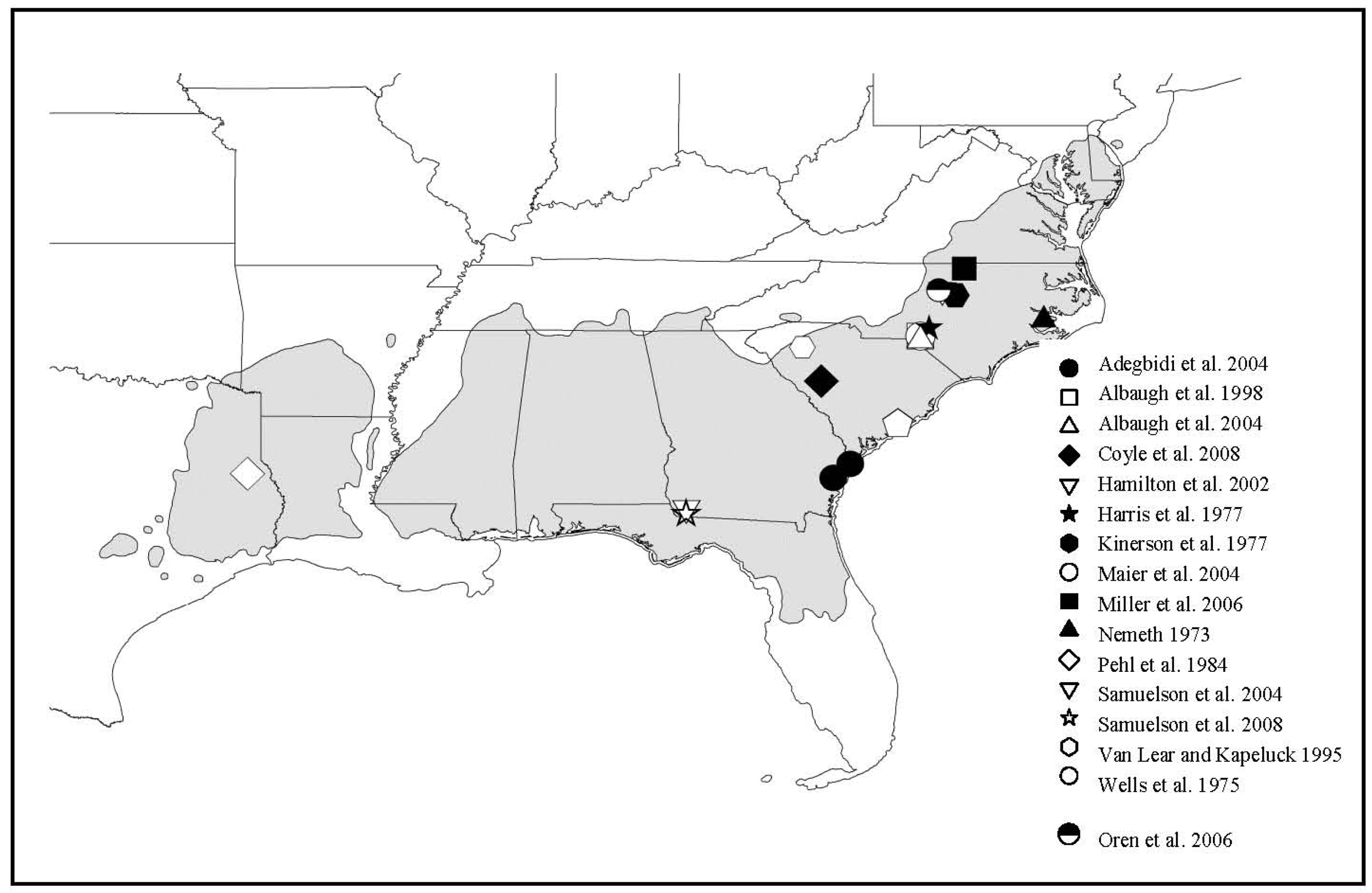
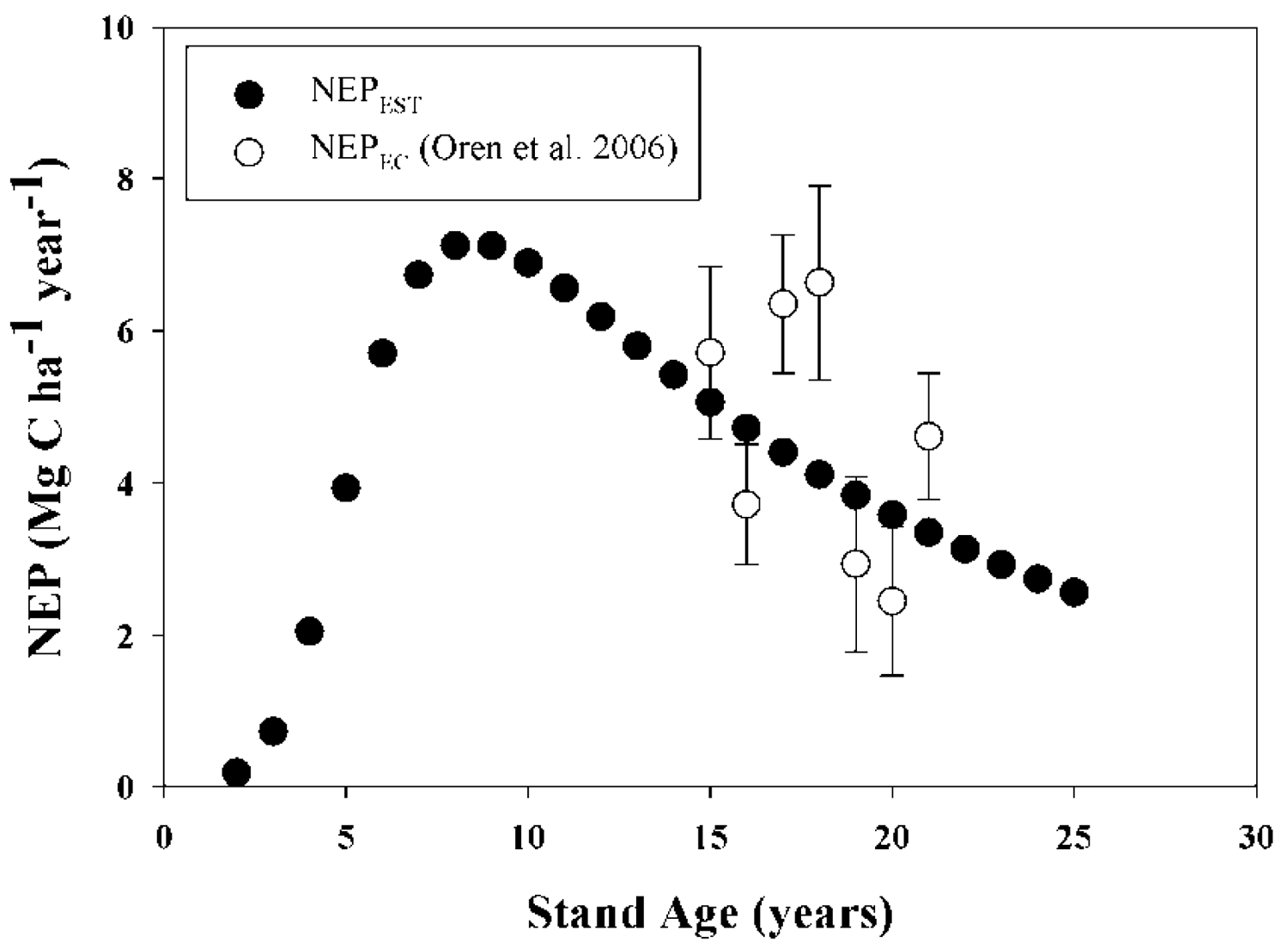
Validation of model results was carried out by comparing model outputs against data reported in the peer-reviewed literature for: (i) total above-plus belowground C accumulation in loblolly pine biomass (TC, MgC·ha−1); (ii) aboveground C accumulation in live loblolly pine biomass (AGC, MgC·ha−1); (iii)belowground C accumulation in live loblolly pine biomass (BGC, MgC·ha−1); and (iv) net ecosystem production (NEP; MgC·ha−1·year−1). Results reported in 15 publications including both above- and belowground loblolly pine biomass, for stands between 3 and 48 years old, were considered in our approach. On each validation study, the authors estimated biomass directly using inventory and local biomass functions. For each literature value, the reported initial stand characteristics such as planting density, SI and management activities (site preparation, weed control, fertilization and thinning) were used as model inputs. Loblolly pine's TC, AGC and BGC were validated in two ways, depending on the availability of information: (i) whole-model validation, using reports that included planting density, SI and management activities [25,41-48]; or (ii) allometry validation, using reports where SI was not reported [27,49-53]. The former enabled us to run the model from planting year to age when biomass was determined. For allometry validation from papers which did not report initial stand characteristics, initial model inputs were adjusted to achieve the final stand characteristics of each report, such as Hd, DBH, BA, Nha. The latter approach can be considered a validation of the biomass equations used by the model. Even though two of the studies used for validation [21,23] utilized some of the equations included in the model (see Table 1), we contend that the independent estimation of Nha, DBH and all other C pool components validate the inclusion of those cases. The values of NEP reported by Oren et al. [54] for 16 to 21-year old stands were compared with our model estimates. A summary table of all data used for C accumulation validations is reported in Appendix 1. Locations of validation sites are also shown in Figure 1. Validation of litterfall and forest floor outputs were developed/tested in related research by Gonzalez-Benecke, et al. 2011 [24]. Validation simulations were performed with the growth and yield functions appropriate for the physiographic region of each validation study.
2.3. Ex Situ Wood Products Pools
Depending on stem DBH and merchantable diameter, harvested roundwood (from thinnings or clear-cuts) was assigned to three main product classes: sawtimber (ST), chip-and-saw (CNS) and pulpwood (PW), using the model proposed by Harrison and Borders [16]. Merchantable outside-bark stem volume was calculated at each stand age and product volume was transformed to biomass (Mg· ha−1) by multiplying the volume by the average specific gravity (SG) at a given age from equations derived from the model [7]. The exponential model that correlates SG and age is shown in Table 1. A C content of 50% was used to calculate C mass of each product type.
Similar to Gonzalez-Benecke et al. [14], industrial conversion efficiencies of 65%, 65% and 58% were assigned to ST, CNS and PW, respectively [25,40,55]. In addition, all the product types were divided into four life span categories (Table 2) [12,56] and adapted to loblolly pine utilization patterns in the southeastern U.S. [57-60].
2.4. Silvicultural Management Scenarios
The effects of silvicultural treatments and rotation lengths on C sequestration were analyzed by simulating C flux under four different scenarios for standard conditions of loblolly pine plantations established in the southeastern US lower Coastal Plain. Initial variables were set as follow: base SI = 22 m, Nha = 1500 trees·ha−1, bedding, weed control at planting and at age 1, and NP fertilization at age 5 (135 Kg·ha−1 N + 28 Kg·ha−1 P), 10 (225 Kg·ha−1 N + 28 Kg·ha−1 P) and 15 years (225 Kg·ha−1 N + 28 Kg·ha−1 P). After fertilization and weed control treatments, the model estimated that the effective SI was increased to 24.3 m. Initial C accumulated from the previous rotation in coarse root debris (∼21.6 MgC·ha−1; [41,42,49]) and the forest floor and aboveground coarse woody debris (∼33.83 MgC·ha−1; [61]) was assumed to be 55.4 MgC·ha−1. This value was similar to the amount of 60.0 MgC·ha−1 reported for a slash pine plantation following a clearcut harvest [62]. Thinning intensity removal was set at 33% of the living trees. Details of the four management scenarios used in the modeling effort are shown in Table 3. Silvicultural-scenario simulations were performed with the growth and yield functions for the lower Coastal Plain physiographic region.
2.5. Carbon Emissions of Transportation and Silvicultural Activities
Emissions of C by silvicultural activities were determined from Markewitz [63] and White et al. [64]. Carbon release in transportation of raw material from the forest to the mill was estimated according to White et al. [64], assuming an average haul distance of 100 km from the forest to the mill, load per logging truck of 24 m3, and fuel economy of the diesel logging truck of 2.6 km 1−1. Details of C emissions are presented in Table 4.
2.6. Sensitivity Analyses
Sensitivity analyses were carried out to determine the effects of changes in key parameter estimates on total C balance. The effects of site quality were assessed by evaluating the model under contrasting SI values of 15 and 30 m, which corresponded to the full range of site qualities observed in loblolly pine plantations in the southeastern US. After fertilization and weed control treatments, the model estimated that the effective SI increased from 15 to 18.2 m, and from 30 to 32.3 m. Initial stand density effects were evaluated by running the model under contrasting planting densities of 750 and 2250 trees·ha−1. Forest floor accumulation and total net C stock were evaluated by using decomposition rates of 10 and 20%; values beyond the extremes of 12 and 17% reported for this region [26,27,65]. In addition to the silvicultural management scenarios tested, rotation length effects were assessed by evaluating the model under the PP scenario for 18 and 35 years. Average product life span was evaluated by changing the proportion of products in different life span classes. In the case of ST and CNS, the proportion of products in the long life classes (50 years) were changed by 25% (step up and down), distributing the residual proportion in equal parts to the rest of the life span classes. Sensitivity analyses to industrial conversion efficiencies were not considered due to their low impact on ex situ C stocks [14].
2.7. Thinning Effects on Loblolly Pine C Stocks
The effects of thinning (as a percentage of living trees removed) were assessed by evaluating the model under different combinations of thinning age (8, 12 and 16 years) and intensity (20, 40 and 60% of living trees removal). Stand and management characteristics were set as those described previously for ST1 (i.e., base SI = 22 m, N = 1500 trees·ha−1, bedding, weed control at planting and at age 1, and NP fertilization at age 5–10–15 years).
2.8. Comparison Between Loblolly and Slash Pine C Stocks
We compared estimates of loblolly pine C stocks with those of slash pine using a previously reported model [14] that was updated with relationships used to estimate LAI, litterfall and forest floor accumulation [24]. Initial parameter estimates such as site index, planting density, site preparation, weed control, fertilization and rotation length were set equal for both species. An analysis for unthinned stands with rotations length of 22 and 35 years was performed. For both species, two NP fertilizations were set at ages 5 and at age 10 years (120 kg·ha−1 diamonium phosphate + 210 kg·ha−1 urea, and 120 kg·ha−1 diamonium phosphate + 430 kg·ha−1 urea, respectively).
2.9. Model
Net C stock was defined as: Net C stock = Total C in situ (C stored in living loblolly pine trees + understory + forest floor + coarse woody debris + standing dead trees) + Total C ex situ (C stored in wood products ST + CNS + PW) − Total C cost (silvicultural activities, including transportation of supplies). For all simulations, estimates of average C stock were reported as the average of all yearly values from the first ∼200 years of management, stopping the simulation at the end of the rotation closest to the 200 year endpoint (not stopping the simulations midway into a rotation). For the scenarios with rotation length of 18, 22 and 35 years, the number of rotations simulated was 11, 9 and 6, respectively. This simulation length was chosen to be sufficiently long to approach steady state values for ex situ pools, while remaining within plausible bounds for consideration of future forest management scenarios. While it is likely that “true” steady state would be achieved for simulations of 500–1000 years, these time periods are far beyond the time horizon over which forest management planning occurs.
2.10. Statistical Analysis
Four measures of accuracy were used to evaluate the “goodness of fit” between observed and predicted (simulated) values for each variable from the dataset obtained in the model validation [66-70]: (i) Mean absolute error (MAE); (ii) Root mean square error (RMSE); (iii) Mean bias error (Bias); and (iv) Pearson product-moment correlation coefficient (R).
3. Results
3.1. Model Validation
There was no statistical difference between average NEP modeled (NEPEST) and measured NEP (NEPEC) from ages 15 to 21 years (P = 0.77), averaging 4.46 and 4.63 MgC·ha−1·year−1 for NEPEST and NEPEC, respectively (Table 5; Figure 2). Predicted values were in the mid-range of variation of observed values.
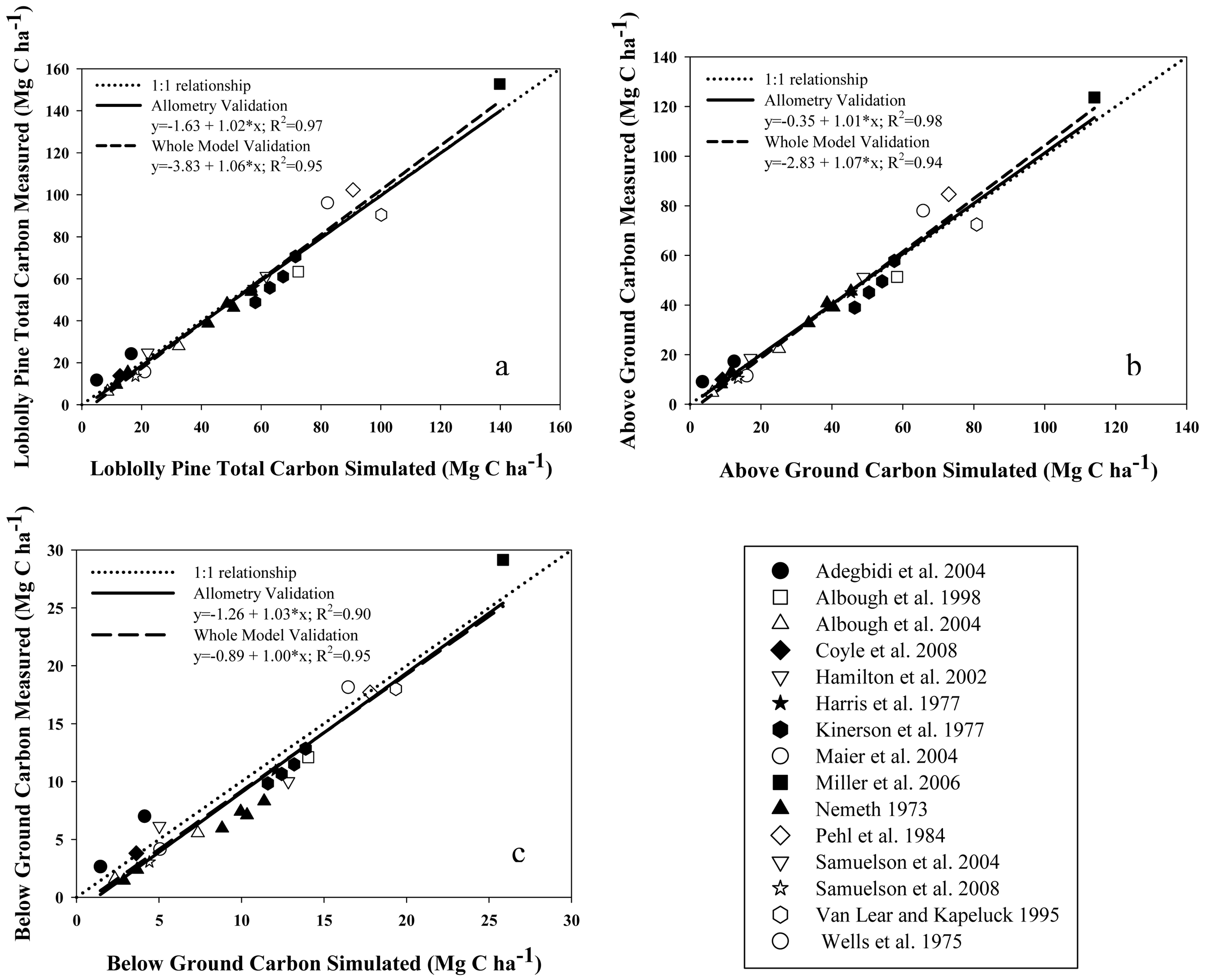
Estimations of C stock in aboveground (AGC), belowground (BGC) and total (TC) live pine were well correlated with values reported for stands of different ages and productivity (R2 > 0.94; Figure 3a, b and c). In all cases, the intercept and slope of these relationships were not different from zero and one, respectively (P > 0.27).
All model performance tests showed that NEP, TC, AGC and BGC estimations agreed well with measured values (Table 5). For the whole-model validation of C stock estimations, MAE and RMSE ranged between 15.3 to 16.7%, and 12.8 to 14.3% of the observed C stock values, respectively. On the other hand, MAE and RMSE for the validation of the allometric equations for biomass estimation (that was carried out with sites were SI was not reported), ranged between 11.1 to 23.2%, and 8.6 to 21.4% of the observed C stock values, respectively. In all cases, BGC estimations presented the larger differences between the observed and predicted values. The Bias of the validation of allometry ranged between 1.5% under-estimations for AGC to 6.5% over-estimations for BGC, whereas Bias for the whole-model validation ranged between 0.1% under-estimations for AGC to 8.5% over-estimations for BGC, with no clear tendency to under- or over-estimate the results. Estimated and observed values of C stock were highly correlated, with R values greater than 0.94. In the case of NEP, the model was less accurate than the C stock estimates, even though the mean was not different between the observed and predicted values. MAE and RMSE were 28.1 and 30.5 % of the observed values, respectively. The Bias showed a 3.7% underestimation.
3.2. Silvicultural Management Effects on C Sequestration
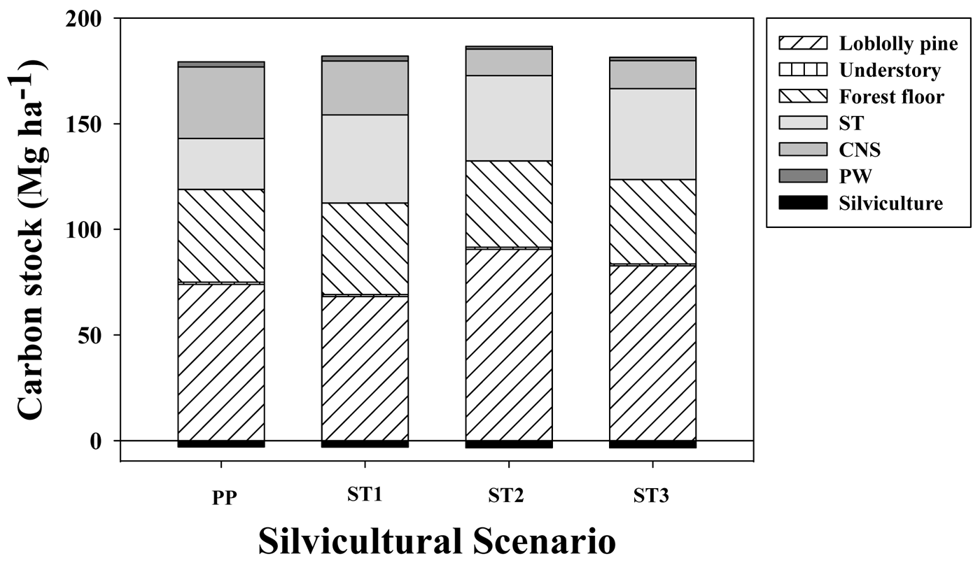
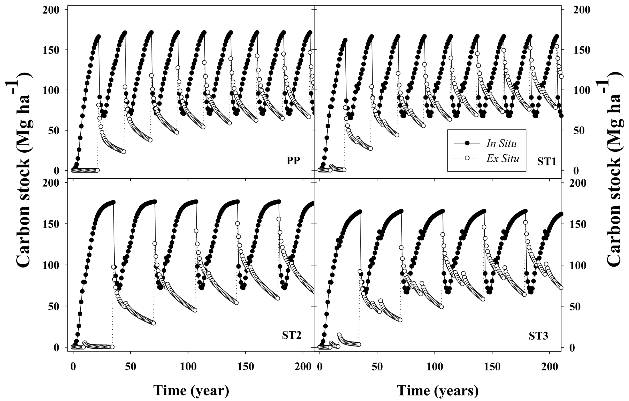
One-thinned or two-thinned stands with longer rotation ages (35 years) stored only 4% or 1% more C, respectively, than unthinned stands harvested at age 22 years. Under conditions used in the simulations, average net C stock, which corresponded to total C in situ (loblolly pine + understory + forest floor + coarse woody debris + standing dead trees) plus total C ex situ (C in woody products ST + CNS + PW) minus total C cost of silvicultural activities (including transport), averaged 176,179,183 and 178 MgC·ha−1 for PP, ST1, ST2 and ST3, respectively, for a 200 year simulation period (Figure 4). In situ C stock accounted for between 62% and 71% of the gross C sequestration (not including silvicultural C costs) across silvicultural regimes. The magnitude of emissions associated with silvicultural activities (including transportation) was between 1.7% and 1.8% of the gross C stock. The relative impact on C sequestration for the different woody products depended on the silvicultural regimes; ST accounted for 40%, 60%, 75% and 74% of total C ex situ for PP, ST1, ST2 and ST3, respectively. In contrast, CNS followed an opposite trend, accounting for 56%, 37%, 23% and 23% for the PP, ST1, ST2 and ST3 silvicultural regimes, respectively. Across different silvicultural management systems, the forest floor + dead trees + coarse woody debris (FFD) components averaged 42 MgC·ha−1 (between 31% to 39% of total in situ C stock) and the understory averaged 1.0 MgC·ha−1 (less than 1% of total in situ C stock).
For a 22-year rotation length, removing 33% of the living trees by thinning at age 10 (ST1) had an almost null effect on average net C stock, increasing C storage by about 2.7 MgC·ha−1. Even though there was a 5.8 MgC·ha−1 reduction in living loblolly pine C stock, there was a 9.1 MgC·ha−1 increment in woody products (mostly due to larger ST production). Extending the rotation age to 35 years with one thinning at age 10 (ST2) increased average net C stock by 4.3 MgC·ha−1 when compared with ST1. The similar C stock between both scenarios was caused mainly by the counteracting effects of larger accumulations in living loblolly pine biomass (22.4 MgC·ha−1 increment) and by a reduction in ex situ C (15.4 MgC·ha−1 decrease). If a second thinning was carried out at age 17 years with the extended rotation scenario (ST3), average net C stock decreased by 5.2 MgC·ha−1, compared with ST2. Most of this decrease was due to lower C accumulation in living loblolly pine (7.8 MgC·ha−1 reduction), which was partially counteracted by an increment in the ex situ C stock of 3.6 MgC·ha−1.
From a total silviculture C cost perspective, fertilization accounted for 0.92 MgC·ha−1 (three fertilizations), representing between 28% and 30% of the total silvicultural C emissions. Harvest and transportation of woody products accounted for between 1.42 and 1.84 MgC·ha−1, representing about 47 to 55 % of the total silvicultural C emissions.
In general, after ∼200 years, C flux in the woody products converged to stable values, reaching quasi-equilibrium minimum and maximum values. At their respective rotation ages, in situ C stocks were 166, 161, 169 and 158 MgC·ha−1 for the PP, ST1, ST2 and ST3 scenarios, respectively (Figure 5). From that total, the C stock in living loblolly pine and the understory was 128, 126, 131 and 124 MgC·ha−1 for the same silvicultural regimes, respectively (data not shown). Total woody products C stock increased each rotation from 80, 77, 95 and 90 MgC·ha−1 during the first rotation, up to 142, 150, 153 and 150 MgC·ha−1 at the end of the rotation closest to the 200 year endpoint, for the PP, ST1, ST2 and ST3 scenarios, respectively (Figure 5). This result implies that in the long term, for extended rotations, C storage fluxes in woody products were similar than the amount of C stored in living loblolly pine.
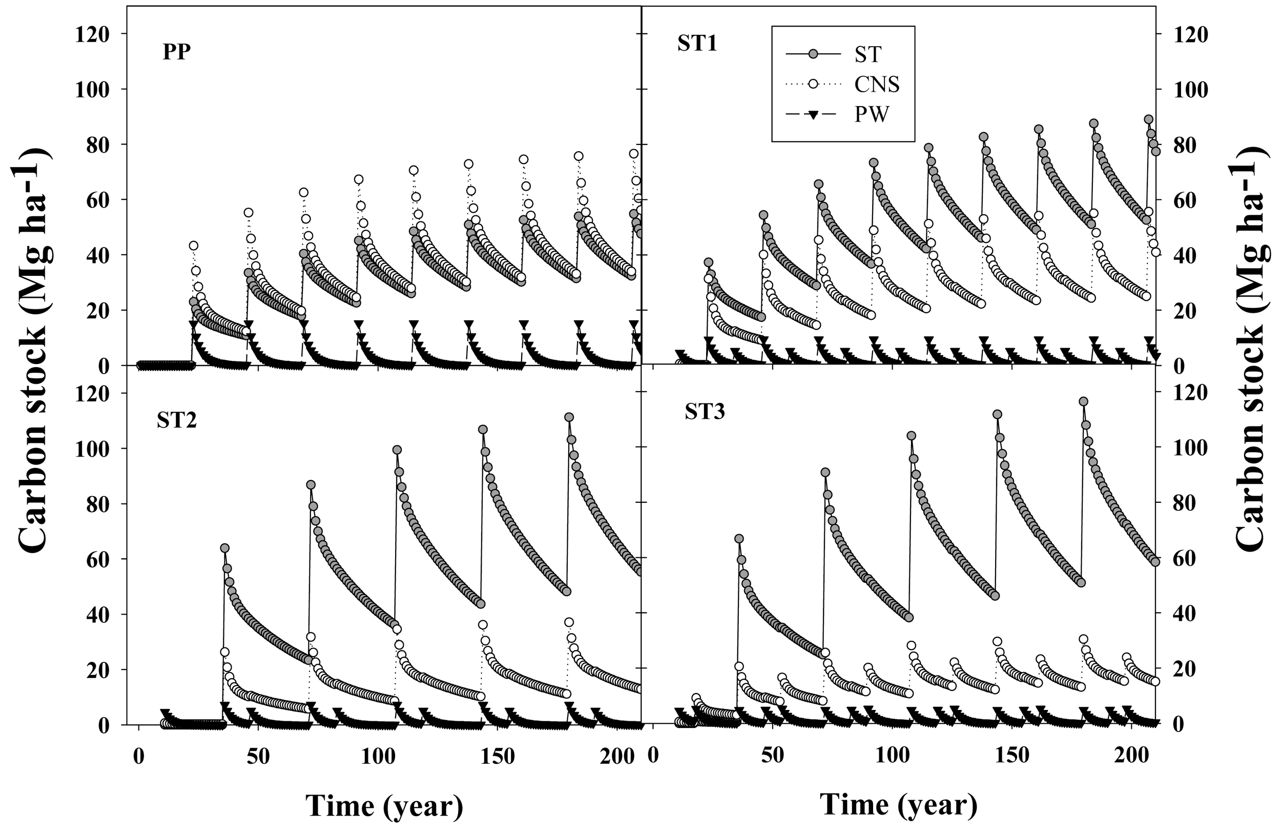
Differences in tree size (diameter and height) and number of trees remaining due to different thinning and rotation age scenarios created different woody products pools that had different life spans. While PW represented 4.2%, 3.4%, 2.3% and 2.6% of the total C extracted in products at harvest, ST accounted for 40%, 60%, 75% and 74% of that C for the PP, ST1, ST2 and ST3 scenarios, respectively. In general, C stored in products derived from PW (e.g., paper, packing material, office supplies, etc.) had a negligible effect on net C sequestration; between harvest events (thinning or clear cutting) the amount of C stored in products derived from pulpwood diminished towards zero, while C stored in CNS and ST increased between harvests (Figure 6).
3.3. Sensitivity Analysis
With all other parameters held constant, site quality (or potential productivity) reflected in SI of the stand, was the major factor controlling C sequestration (Table 6). For example, on low productivity sites (e.g., base SI = 15 m), average net C stocks were about 28% lower than with the default site quality (base SI = 22 m). In contrast, for high quality sites (e.g., base SI = 30 m), C stocks across silvicultural regimes averaged about 38% greater than base SI = 22 (Table 6). When SI was set equal to 15 m, ex situ C stocks were largely reduced for sawtimber-oriented silvicultural regimes. In situ C stocks were reduced 21.6, 20, 25.6 and 24 MgC·ha−1, and ex situ C stocks were reduced 28, 30, 26.4 and 26.8 MgC·ha−1, for PP, ST1, ST2 and ST3, respectively. By comparison, for base SI = 30 m, in situ C stocks increased 25, 23, 30 and 28 MgC·ha−1, and ex situ C stock augmented 44.6, 44.7, 39.3 and 40 MgC·ha−1, for the PP, ST1, ST2 and ST3 management regimes, respectively. The silvicultural treatments included in our analysis, that improved SI by 3.2, 2.3 and 2.3 m, for stands with base Si of 15, 22 and 30 m, respectively, produced an increase in net C stock of 12.5, 12.4 and 12.8 MgC·ha−1, respectively, across management regimes (Table 6).
The effects of planting density were largely reflected in in situ rather than ex situ C pools. Reducing the initial planting density decreased net C stocks up to 10%, while increasing the planting density enhanced net C stocks by about 6% among silvicultural regimes. By lowering planting density from 1500 trees·ha−1 to 750 trees·ha−1, the average net C stocks decreased 16.6,17.3,19 and 18.9 MgC·ha−1 for the PP, ST1, ST2 and ST3 management systems, respectively. This reduction was explained principally by a decrease in the in situ C stocks of 11.7, 10.5, 10.7 and 10.3 MgC·ha−1 for the same silvicultural regimes. The effects on ex situ C stocks were substantially smaller, producing gains of 2.4 MgC·ha−1 for the PP, but reductions of 0.1, 2.2 and 3.1 MgC·ha−1 for the ST1, ST2 and ST3 management systems, respectively. By increasing the initial planting density from 1500 trees·ha−1 to 2250 trees·ha−1, average net C stocks were increased 10.7, 9.5, 11.2 and 11 MgC·ha−1 compared to the default initial planting density for the PP, ST1, ST2 and ST3 treatments, respectively. For the high initial planting density, in situ C stocks were increased 8.1, 7.2, 6.8 and 6.6 MgC·ha−1 for the PP, ST1, ST2 and ST3 silvicultural management systems, respectively. The C storage in woody products was reduced by 2.7, 2.4 MgC·ha−1 for the PP and ST1 management regimes, but was increased by 0.2 and 0.7 MgC·ha−1 for the ST2 and ST3 scenarios, respectively.
Shortening the rotation length to 18 years under the PP scenario (unthinned), which corresponded to the biological rotation age for that silvicultural scenario (i.e., the time when mean annual increment equals periodic annual increment), reduced the average net C stock to 164.2 MgC·ha−1. This 7% decrease, when compared with the default 22-year-rotation, was caused mainly by reductions in the in situ rather than ex situ C stocks (10.8 and 1.4 MgC·ha−1 reductions, respectively). When the rotation age was extended to 35 years, average net C stocks increased to 183.2 MgC·ha−1.
When the C decay rate was reduced to 10% or increased to 20%, average net C stocks increased or decreased between 7.5 and 6.6%, respectively, across silvicultural regimes (Table 6). Assuming a decay rate of 10%, C storage in the FFD increased to about 13.3 MgC·ha−1, across silvicultural regimes, compared to a decay rate of 15%. When the decay rate was increased up to 20%, the C stocks in the FFD were reduced to about 11.8 MgC·ha−1.
Variations in average life span of ST and CNS woody products affected net C stock. On the other hand, paper product life span had a smaller effect on net C storage (Table 6). When the average life span of ST was increased by increasing the product proportion in the long-lived class (half-life 50 years, Table 2) from 50% to 75%, average net C stocks were increased 7.3, 12.6, 11.9 and 12.6 MgC·ha−1 for the PP, ST1, ST2 and ST3 management regimes, respectively; this represented an increment of between 4.1 and 7.1% (Table 6). On the other hand, when the ST proportion of long life span products was stepped-down to 25%, reductions in C increments of the same magnitude were observed. The impact of the CNS half-life on net C stocks was more important in the PP than the sawtimber-oriented regimes, changing average net C stocks by 12.2, 9.2, 4.3 and 4.6 MgC·ha−1 for the PP, ST1, ST2 and ST3 management scenarios, respectively (Table 6). When all PW products were set to have a life span of one year, average net C stocks was reduced between 0.42 and 0.86 MgC·ha−1. Conversely, when the PW products life span was increased by assuming that 67% of PW products would have a life span of four years, the average net C stock was increased between 0.45 and 0.89 MgC·ha−1.
3.4. Thinning Effects on Loblolly Pine C Sequestration
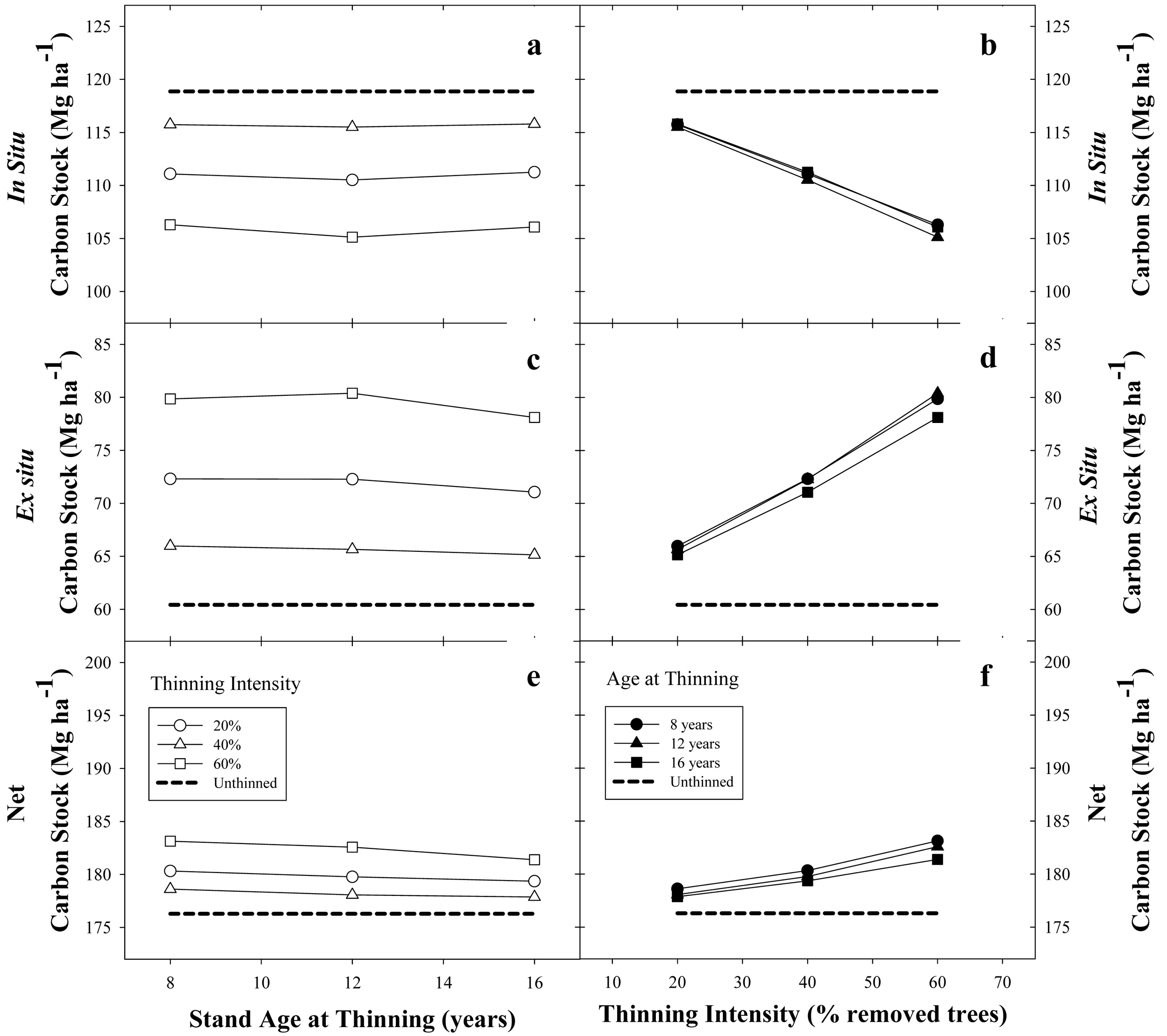
In general, for a base SI = 22 m stand with 1500 trees·ha−1 and managed under a 22-year rotation, thinning had a positive on net C stock. The negative effect of thinning on the in situ C stock was largely counteracted by increasing the ex situ C stock, producing an increase in average net C stock (Figure 7).
For any given thinning intensity, there was a small effect due to the age of thinning on the in situ C stock (Figure 7a). For example, using a thinning intensity of 20% at ages 8, 12 and 16 years reduced the in situ C stock by 3.1, 3.4 and 3.1 MgC·ha−1, respectively (Figure 7a). Increments in thinning intensity produced a quasi-constant decline in in situ C stock, independent of thinning age. For instance, in situ C stocks were reduced 3.2, 7.9 and 13 MgC·ha−1, when thinning intensities were set at 20, 40, and 60% removal of living trees, respectively (Figure 7b). Ex situ C storage had an opposite response to thinning; the more intensive the thinning regime, the more gain in woody products C storage. Ex situ C storage was slightly increased by thinning age for any given thinning intensity. For example, when thinning age was set at 8,12 and 16 years, with a thinning intensity of 20%, the ex situ C stock was increased by 5.6, 5.2 and 4.7 MgC·ha−1, respectively; when thinning intensity was set to 60%, ex situ C stocks were increased 19.4, 19.9 and 17.7 MgC·ha−1, respectively (Figure 7c). Increments in thinning intensity produced a quasi-constant increment in ex situ C stock independent of thinning age. Ex situ C stocks were increased 5.2, 11.5 and 19 MgC·ha−1, when thinning intensities were set at 20, 40 and 60% removal of living trees, respectively (Figure 7d). Due to the larger positive effects on ex situ C storage, rather than smaller negative effects on in situ C storage, net C stocks were slightly increased by thinning (Figure 7e and f).
3.5. Comparison in C Sequestration between Loblolly and Slash Pine Stands
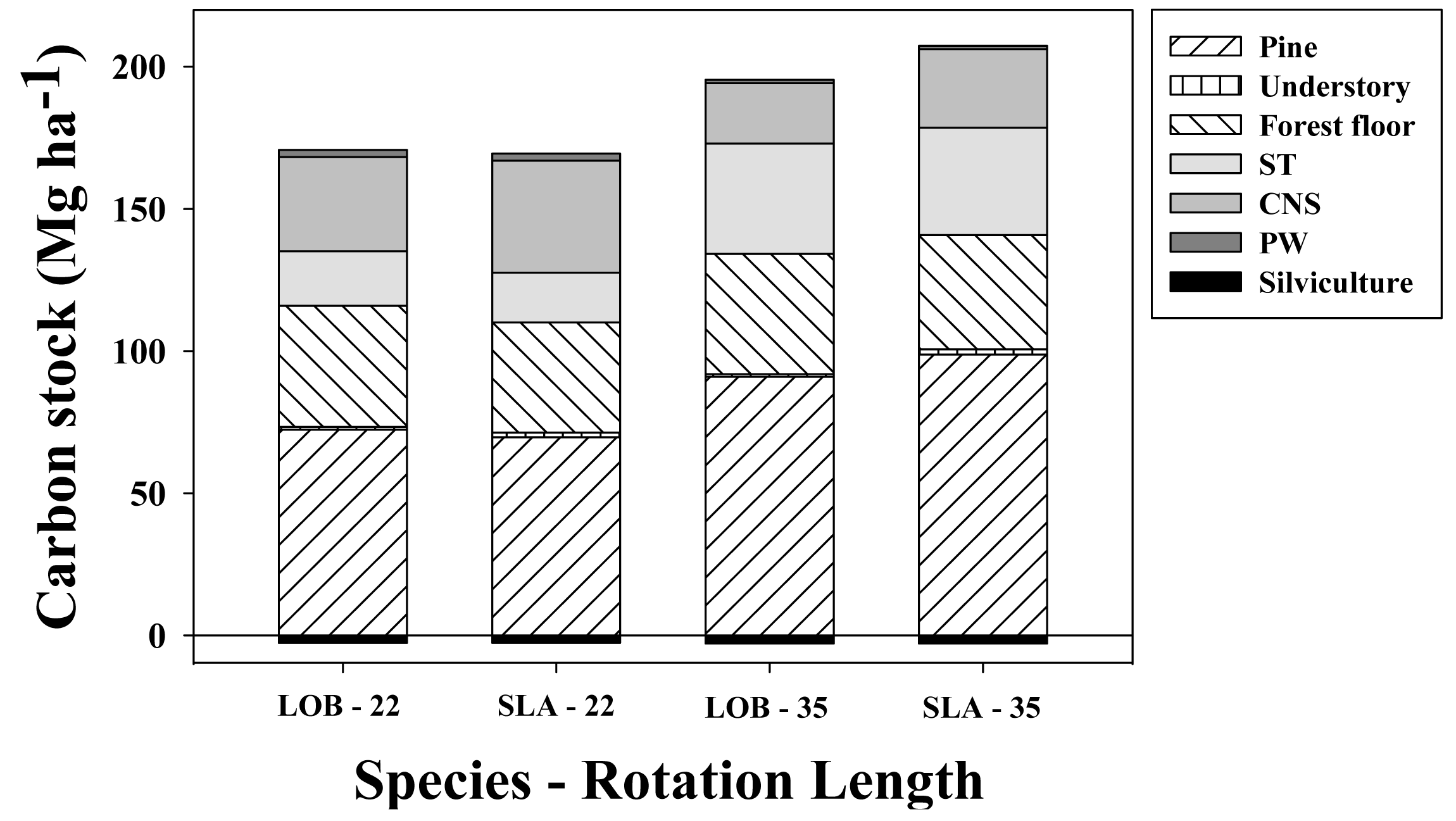
Under the default parameters used for simulations in unthinned loblolly pine stands harvested at age 22 years, loblolly and slash pine net C stocks were generally similar, albeit on an absolute basis loblolly pine accumulated 1.3 Mg·ha−1 more C than slash pine (Figure 8). This 1% difference in favor of loblolly pine was explained mainly by increases in stored C in the living tree biomass (2.8 MgC·ha−1) and FFD (3.8 MgC·ha−1) pools. It should be noted, however, that a 4.6 MgC·ha−1 decrease in the loblolly pine woody products pool partially counteracted that gain. Understory biomass was 0.7 MgC·ha−1 larger in slash pine than in loblolly pine stands. When the rotation length was increased to 35 years without thinning, slash pine C stocks exceeded loblolly pine, averaging 11.9 MgC·ha−1 more net C stock. This difference was explained mainly through increases in net C stored in the living tree (7.8 MgC·ha−1) and ex situ biomass (5.3 MgC·ha−1) pools. Understory C accumulation was 0.9 MgC·ha−1 larger in slash pine than in loblolly pine stands, and the FFD was 2.1 MgC·ha−1 larger in loblolly than in slash pine stands.
4. Discussion
Loblolly pine plays an important role in mitigation of CO2 emissions due to its high productivity and extensive planting throughout the southeastern U.S. Accurate determinations of C stocks and the understanding of factors controlling C dynamics in loblolly pine plantations are essential for C offset projects and the development of sustainable management systems. To validate the model predictions, we utilized 15 peer-reviewed publications that reported estimates of both above and belowground biomass accumulations in loblolly pine stands. Several other publications were also found that reported only aboveground biomass estimates ([71-75], among many others); however, we decided to validate the model using only those published studies that included both above- and below-ground estimates measured at the same time for a given site. Further, the model was tested on stands of contrasting site quality (SI ranges between 15.5 to 32 m) that ranged in age from 3 to 48 years, across different physiographic regions that cover the planting range of the species (Figure 1; Appendix 1). The strong agreement between observed and predicted values supported the robustness of the model and its usefulness for assessing the effects of forest management activities on C sequestration (in situ, and ex situ) for the most important commercial tree species in the southeastern US.
The dominant factor controlling C sequestration in loblolly pine plantations was site quality as it interacted with different management scenarios. Similar responses have been reported for slash pine [14], Pinus radiata D. Don and Pinus pinaster Ait. [76]. Across the silvicultural regimes evaluated there were similar changes in in situ C stocks, but ex situ C storage was largely affected by site quality changes and longer rotation lengths oriented toward sawtimber production. Specifically, our results indicated that: (i) long rotation oriented-sawtimber silvicultural regimes were not as effective for C storage on low quality sites, but they were more effective on high quality sites; and (ii) ex situ carbon pools were important considerations when evaluating the C offset potential of different management systems. Over the past 50 years, the productivity of planted loblolly pine stands has tripled [9,77], implying an important effect of modern forest management systems (interaction between genetic improvement, seedling culture, and nutrient and competition management) not only on volume yield, but also on total C storage. The rate of development and implementation of technology that increases production rates will determine the contribution of future plantation C storage. The effects of site quality changes in C storage were exacerbated by the effects of ex situ C sequestration because increases in site quality not only increased total standing volume (or stand biomass), but also increased the proportion of trees making valuable product grades that had a long life span.
Increasing initial planting density in the range tested in this study had a positive effect on net C storage, and the effects of planting density on C storage were most apparent in the in situ C pool, affecting both living tree biomass and FFD biomass accumulation. Even though raising the planting density increased the proportion of fixed C used in stem production in loblolly pine [78], this effect was not reflected in the ex situ C pool. As planting densities increased, there was a tendency to decrease sawtimber products yields, affecting the average ex situ C pools; however, the increase in forest floor, coarse woody debris and total living tree C storage largely counteracted that negative effect. Morton [79] concluded that utilizing higher planting densities maximized C sequestration and with a market value for C credits, land expectation values were maximized by utilizing higher planting densities as well.
Increasing the rotation length increased C stock in loblolly pine stands. We estimated similar net increments of 6.9 MgC·ha−1 when rotation lengths were increased from 22 to 35 years for unthinned and thinned stands. Most of this increment was accounted for in the in situ C storage. In contrast, when rotation lengths were shortened to 18 years, net C stock was reduced. Other reports for different conifer species [12-14] indicated similar effects of rotation length on C storage i.e., extended rotations increased C sequestration in conifer forest plantations. Longer harvesting cycles represent one of the major management strategies used to increase forest C density [80]. Nevertheless, the inclusion of biomass harvest for fossil fuel offset might change our conclusions, especially when shorter rotations include provisions for a technology bump at the end of each rotation. Further research is needed in this area, and this model is a tool to address these types of questions.
In our study, under a low decomposition rate of 10%, the C stock in the FFD increased about 13.3 MgC·ha−1; under a higher decomposition rate of 20%, C stocks in the FFD decreased about 11.8 MgC·ha−1. As changes in soil temperature and moisture regimes can affect litter decomposition rates [81], it is probable that future environmental changes would be expected to alter litter decomposition rates in loblolly pine stands, and thereby affect the C storage capacity of the forest.
When stand C density was compared between loblolly and slash pine stands under similar levels of site quality (base SI = 20 m) and silvicultural inputs over a 22-year rotation length, living pine C stocks of loblolly and slash pine were generally similar (loblolly pine was 1% greater than slash pine). Under longer rotations (i.e., 35 years), the average net C stocks of both species remained similar; however, slash pine was about 6% greater than loblolly pine. For thinned stands with similar SI as our simulations, loblolly pine at age 31 years had about 8% more standing volume than slash pine [82]. For unthinned stands at age 28 years, the differences between loblolly and slash pine standing volumes were about 1% [83]. The first study to our knowledge that compared C stocks between southern pine species in mature stands was from Vogel et al. [84]. The authors reported that at age 26 years, living tree C stocks of loblolly pine were larger than slash pine when nutritional limitations were eliminated through fertilizer additions. Under nonfertilized conditions, even with sustained elimination of understory vegetation, living tree C stocks were larger for slash pine than for loblolly pine. As nutritional demands and the responses to fertilization for loblolly pine tend to be larger than slash pine [77], differences in nutrient requirements and nutrient use efficiency between the two species should be taken in account when developing sustainable and ecological forestry regimes. In our analysis, the fertilization regime included two applications, which may not be sufficient to support the demands of loblolly pine, especially under longer rotations scenarios.
For the ∼200 year simulation period, thinning decreased in situ C stocks, but increased ex situ C stocks more, resulting in slight increases in net C stocks. Most of the studies that have addressed the impacts of thinning on C budgets in pine ecosystems have reported the responses only on living pine biomass [76,85-88]; few studies have reported the impacts of thinning on total in situ C [89-92]. All the previously cited studies concluded that there was a reduction in pine stand or total in situ C after thinning. The negative effects of thinning were also reported for NEP fluxes for Pinus ponderosa Dougl. forests [90,91]. In both studies, the authors reported a decrease in NEP for thinned stands. To our knowledge, the current study represents one of the few that incorporated the ex situ C pool into the analysis of thinning effects on carbon sequestration of forest plantations. Garcia-Gonzalo [93], in a similar analysis that included ex situ C pools for mixed coniferous stands in Finland, reported a net reduction between 25 and 33 MgC&midotha−1 in trees and a net increase between 30 and 45 MgC·ha−1 in harvested timber. Even though the wood extracted in thinning was primarily pulpwood, which impacted ex situ C sequestration, increased growth of residual trees due to thinning promoted the production of larger tree size classes at final harvest. These long-lived products increased the ex situ C pool, overcompensating for the reduction in in situ C associated with thinning. When ex situ pools were considered, the possible economic benefits of thinning were not in opposition to maintaining or increasing net C stock. This, and other evidence, suggests that there is no simple inverse relationship between the amount of timber harvested from a forest and the amount of C stored [94].
It should be noted that estimates of the effects of scenarios on net C stocks are somewhat sensitive to the length of simulation. This is because ex situ C stocks take centuries to reach equilibrium levels (200–400 years for the scenarios we tested, data not shown). Therefore, as longer and longer simulation periods are compared, the effects of differences in in situ C stocks on net C stocks tend to be dampened by converging magnitudes of ex situ C stocks. This makes it important to carefully consider the inference space desired for a particular simulation. For relatively short-term management decisions, it may be appropriate to run simulations for only one or two rotations. For decision-making associated with C offset accounting contracts, 50–150 years may be appropriate. As mentioned previously, we chose 200-year simulations as a length of time long enough to allow development of near-equilibrium ex situ stock levels, but not so long that the time period moved out of the realm of realistic forest management planning.
Under the Intergovernmental Panel on Climate Change [95], reporting of C stock in wood products is not mandatory, but the enhancement of that C pool could provide important GHG emission offsets. Results from this study suggested that extending the half-life of PW products had only a marginal effect on C stock. Similar results were reported in other studies [14,56,58]. The ex situ C pools could be influenced by both the final utilization of particular products, and also by substituting wood for more C intensive materials. If waste wood and forest biomass residues were used as substitutes for fossil fuels [96], or if long lasting wood products took the take the place of more C intensive materials like concrete or steel [97], then the mitigation impacts of ex situ C stocks could be even larger.
5. Conclusions
In this article we provide a model for quantifying C sequestration for loblolly pine plantations under varying management conditions in the southeastern U.S. Coastal Plain and Piedmont regions. The model performed accurately when it was tested against reported C measurements over a wide range of stand ages and site qualities. Using the model to evaluate the effects of silvicultural management systems on C sequestration over a 200 year simulation period, we conclude that: (i) site quality (productivity), that can be altered by silviculture and genetic improvement, represents the major factor controlling average net C stock in loblolly pine plantations; (ii) if woody products were incorporated into the accounting, thinning tends to be C positive because of the larger positive effects on ex situ C storage; (iii) shorter rotations (biological rotation age) were not as effective for C sequestration as extended rotations that increased average net C stock; (iv) C sequestered in woody products accounted for ∼34% of the net C stock; (v) changes in decomposition rates associated with possible global climate change could affect C storage capacity of the forest; and (vi) emissions due to silvicultural and harvest activities were small compared to the magnitude of the total stand C stock.


| Component | Equation | Source | |
|---|---|---|---|
| BF | If DBH < 26 cm: ln(BF) = −3.982 + 1.010 × ln (DBH2) | Jokela and Martin 2000 | [20] |
| If DBH ≥ 26 cm: log10(BC) = 1.927 + 1.567 × log10 (DBH) | Naidu et al. 1998 | [19] | |
| BB | If DBH < 26 cm: ln(BF) = −5.024 + 1.357 × ln (DBH2) | Jokela and Martin 2000 | [20] |
| If DBH ≥ 26 cm: log10(BC) = 1.122 + 2.308 × log10 (DBH) | Naidu et al. 1998 | [19] | |
| BC | BF + BB | ||
| BS | If DBH < 26 cm: ln(BS) = −3.651 + 1.342 × ln (DBH2) | Jokela and Martin 2000 | [20] |
| If DBH ≥ 26 cm: log10(BAG) = 1.333 + 2.708 × log10 (DBH) | Naidu et al. 1998 | [19] | |
| BAG | If DBH < 26 cm: ln(BAG) = −2.886 + 1.284 × ln (DBH2) | Jokela and Martin 2000 | [20] |
| If DBH ≥ 26 cm: log10(BAG) = 1.830 + 2.464 × log10 (DBH) | Naidu et al. 1998 | [19] | |
| BTR | log10BTR = −2.2760 + 1.742 × log10 (DBH) | Samuelson et al. 2004 | [21] |
| BCR | log10BCR = −4.9500 + 2.211 × log10 (DBH) | Samuelson et al. 2004 | [21] |
| BFR | If Age ≤ 4 years: | Adegbidi et al. 2004 | [23] |
| If Age > 4 years: BFR = 0.202594 × BF* | Samuelson et al. 2004 | [21] | |
| LAI | LAI = β0/(1 + exp(−(SDI − β0)/ β1)) | Gonzalez-Benecke et al. 2011 | [24] |
| β0 = −2.01424307 + 0.19323226 × SI | |||
| β1 = 23.4519 + 2.1389 × SI | |||
| β2 = 327.2346/[1 + (SI / 18.5717) −4929] | |||
| BN | ln (BN) = 0.62455 + 0.97146 × ln(LAI*) | Gonzalez-Benecke et al. 2011 | [24] |
| BN/BL | For stands without weed control at planting and Age <10 years: | Gonzalez-Benecke et al. 2011 | [24] |
| BN/BL = 0.0005 × Age3 − 0.022 × Age2 + 0.2592 × Age − 0.0122 | |||
| For stands without weed control at planting and Age >10 years; for stands with weed control at planting at any age: | |||
| BN/BL = 1/ (0.96294 + 0.019426 × Age − 0.000262 × Age2) | |||
| BU | BU = (0.88242377 + 14.925223)/(1 + 1.5801704 × LAI + 0.8650196 × LAI2) | Gonzalez-Benecke et al. 2010 | [14] |
| SG | SG = 0.3758081 × Age0 0821216 | Harrison and Borders 1996 | [16] |
Note: BF is foliage biomass (kg·tree−1); BB is branch biomass (kg·tree−1); BC is crown biomass (kg·tree−1); BS is stem plus bark biomass (kg·tree−1); BAG is aboveground biomass (kg·tree−1); BTR is tap root biomass (kg·tree−1); BCR is coarse root biomass (kg·tree−1); BFR is fine root biomass at land area basis (Mg·ha−1); BF* is foliage biomass at land area basis (Mg·ha−1); LAI is mean annual projected leaf area index (m2·m−2); SDI is Reinecke's stand density index in metric units; β0, β1 and β2 are sigmoidal fit parameters; SI is site index (m); LAI* is previous year LAI (m2·m−2); BL is current year needlefall biomass (Mg·ha−1·year−1); BN is current year litterfall biomass (Mg·ha−1·year−1); BU is understory biomass (Mg·ha−1); SG is specific gravity (derived from stem volume and dry weight equations reported by Harrison and Borders 1996); DBH is diameter at breast height (cm); Age is stand age (years).
| Product | Product proportions by life span category (%) | |||
|---|---|---|---|---|
| Long (50) | Medium-long (16) | Medium-short (4) | Short (1) | |
| ST | 50 | 25 | 0 | 25 |
| CNS | 25 | 25 | 0 | 50 |
| PW | 0 | 0 | 33 | 67 |
Note: ST is Sawtimber; CNS is Chip and Saw; PW is Pulpwood; Values in parenthesis indicate average life span for class (years).
| Scenario | Rotation length (years) | Thinning |
|---|---|---|
| 1. Pulpwood production (PP) | 22 | - |
| 2. Sawtimber production short rotation (ST1) | 22 | Th10 |
| 3. Sawtimber production long rotation (ST2) | 35 | Th10 |
| 4. Sawtimber production long rotation (ST3) | 35 | Th10 + Th17 |
Note: Th10 is commercial thinning of 33% of living trees at age 10 yr; Th17 is commercial thinning of 33% of living trees at age 17 yr. All scenarios included bedding, weed control at planting and at age 1, and NP fertilization at age 5, 10 and 15 yr.
| Activity | Description | C use (MgC·ha−1) |
|---|---|---|
| Site Preparation | Raking or spot piling + Weed control (aerial application + product) + Bedding | 0.237 |
| Planting | Machine planting | 0.101 |
| Banded Weed Control | Banded Herbicide (backpack application + product) | 0.091 |
| Initial fertilization (age 5) | 120 kg·ha−1 diamonium phosphate + 210 kg·ha−1 urea | 0.216 (1) |
| Mid-rotation fertilization (age 10 and up) | 120 kg·ha−1 diamonium phosphate + 430 kg·ha−1 urea | 0.350 (1) |
| Thinning | Commercial thinning | 0.156 |
| Final harvest | Clear cutting at rotation age | 0.156 |
| Transportation | Average for 24 m3 load capacity | 0.0026 (2) |
Note:(1)Carbon use in fertilization includes production, packing, transportation and application [63];(2)Carbon use for transportation is expressed in MgC used per m3 transported [64].
| Type of validation | Variable | Ō | P̄ | n | MAE | RMSE | Bias | R |
|---|---|---|---|---|---|---|---|---|
| Whole Model | NEP | 4.63 | 4.46 | 7 | 1.30 | 1.41 | −0.17 | 0.42 |
| AGC | 40.53 | 40.47 | 10 | 5.53 | 6.75 | −0.06 | 0.97 | |
| BGC | 9.65 | 10.47 | 10 | 1.38 | 1.55 | 0.82 | 0.98 | |
| TC | 50.17 | 50.94 | 10 | 6.41 | 7.67 | 0.76 | 0.98 | |
| Allometry | AGC | 36.29 | 36.82 | 16 | 3.11 | 4.17 | −0.53 | 0.98 |
| BGC | 9.76 | 9.12 | 16 | 2.09 | 2.27 | 0.64 | 0.94 | |
| TC | 51.08 | 50.01 | 16 | 4.51 | 5.69 | 1.08 | 0.98 | |
Note: NEP is net ecosystem production (MgC·ha−1·year−1); AGC is loblolly pine aboveground C accumulation (MgC·ha−1); BGC is loblolly pine belowground C accumulation (MgC·ha−1); TC is loblolly pine total C accumulation (MgC·ha−1); Ō is the mean observed value; P̄ is the mean predicted value; n is the number of observations; MAE is the mean absolute error; RMSE is the root of mean square error; Bias is the absolute bias estimator; R is the Pearson's correlation coefficient.
| Parameter | Value | PP(MgC ha−1 %) | ST1(MgC ha−1 %) | ST2 (MgC ha−1 %) | ST3 (MgC ha−1 %) | ||||
|---|---|---|---|---|---|---|---|---|---|
| Default value | 176 | 179 | 183 | 178 | |||||
| Site Index (m) | 15 | 114.5 | −35.1% | 116.9 | −34.7% | 119.4 | −34.8% | 116.2 | −34.7% |
| 18.2 | 127.2 | −27.9% | 129.5 | −27.6% | 131.9 | −28.0% | 128.0 | −28.1% | |
| 22 | 163.9 | −7% | 166.7 | −6.9% | 170.4 | −7% | 165.6 | −7% | |
| 30 | 232.9 | 32.1% | 234.1 | 30.8% | 238.0 | 29.9% | 232.0 | 30.3% | |
| 32.3 | 245.3 | 39.2% | 246.0 | 37.5% | 251.5 | 37.3% | 245.3 | 37.8% | |
| Planting density (trees ha−1) | 750 | 159.7 | −9.4% | 161.6 | −9.7% | 164.2 | −10.4% | 159.2 | −10.6% |
| 2250 | 187.0 | 6.1% | 188.5 | 5.3% | 194.5 | 6.1% | 189.1 | 6.2% | |
| Rotation length (years) | 18 | 164.2 | −6.9% | - | - | - | - | - | - |
| 35 | 183.2 | 3.9% | - | - | - | - | - | - | |
| Decay rate (%) | 10 | 190.6 | 8.1% | 192.6 | 7.6% | 196.1 | 7.0% | 190.6 | 7.0% |
| 20 | 1 64.1 | −6.9% | 166.7 | −6.8% | 171.8 | −6.3% | 166.8 | −6.3% | |
| ST percentage in long lifespan class (%) | 25 | 1 69.0 | −4.1% | 166.3 | −7.1% | 171.4 | −6.5% | 165.5 | −7.1% |
| 75 | 183.6 | 4.1% | 191.6 | 7.0% | 195.1 | 6.5% | 190.7 | 7.1% | |
| CNS percentage in long lifespan class (%) | 0 | 164.1 | −6.9% | 169.7 | −5.2% | 179.0 | −2.3% | 173.5 | −2.6% |
| 50 | 188.5 | 6.9% | 188.2 | 5.2% | 187.5 | 2.3% | 182.6 | 2.6% | |
| PW percentage in medium-short lifespan class (%) | 0 | 175.4 | −0.5% | 156.9 | −0.5% | 185.9 | −0.2% | 180.3 | −0.3% |
| 67 | 177.2 | 0.5% | 158.3 | 0.5% | 186.7 | 0.2% | 181.3 | 0.3% | |
Note: Average net carbon stock (MgC·ha−1) is the average of a ∼200 year simulation period and Δ% is the percentage deviation from default parameter values used (Effective site index = 24.3 m; Planting density = 1500 trees·ha−1 Rotation length = 22 years; Decay rate = 15%; ST in long life class = 50%; CNS in long life class = 25% PW in medium-short life class = 33%).
Acknowledgments
The National Institute of Food and Agriculture funded this research through the Regional Approaches to Climate Change Coordinated Agricultural Project program. The Carbon Resources Science Center at the University of Florida also provided funding. We thank Marshall Jacobson, Plum Creek Timber Company Inc., for his advice on silvicultural prescriptions.
Appendix
| Source | Stand Age | Lat | Long | Physiographic Region | AGC | BGC | NEP | |
|---|---|---|---|---|---|---|---|---|
| Adegbidi et al. 2004 | [23] | 3 | 31.6 | −81.4 | LCP | 9.05 | 2.65 | - |
| Coyle et al. 2008 | [98] | 4 | 33.38 | −81.67 | UCP (SAH) | 10.0 | 3.8 | - |
| Adegbidi et al. 2004 | [23] | 4 | 31.92 | −81.03 | LCP | 17.25 | 7.0 | - |
| Samuelson et al. 2004 | [21] | 6 | 30.8 | −84.65 | UCP | 18.6 | 6.15 | - |
| Albaugh et al. 2004 | [43] | 8 | 34.87 | −79.48 | UCP (SAH) | 4.7 | 1.6 | - |
| Nemeth 1973 | [51] | 8 | 35.33 | −76.75 | UCP | 51.3 | 12.1 | - |
| Nemeth 1973 | [51] | 9 | 35.33 | −76.75 | UCP | 10.45 | 3.05 | - |
| Nemeth 1973 | [51] | 10 | 35.33 | −76.75 | UCP | 11.52 | 4.16 | - |
| Samuelson et al. 2008 | [44] | 11 | 30.8 | −84.65 | UCP | 45.0 | 10.95 | - |
| Albaugh et al. 1998 | [45] | 11 | 34.87 | −79.48 | UCP (SAH) | 51.28 | 10.01 | - |
| Nemeth 1973 | [51] | 11 | 35.33 | −76.75 | UCP | 22.35 | 5.55 | - |
| Nemeth 1973 | [51] | 11 | 35.33 | −76.75 | UCP | 77.975 | 18.15 | - |
| Nemeth 1973 | [51] | 12 | 35.33 | −76.75 | UCP | 123.65 | 29.15 | - |
| Maier et al. 2004 | [46] | 12 | 34.87 | −79.48 | UCP (SAH) | 84.65 | 17.7 | - |
| Kinerson et al. 1977 | [52] | 13 | 35.81 | −78.7 | PED | 72.45 | 18.0 | - |
| Kinerson et al. 1977 | [52] | 14 | 35.81 | −78.7 | PED | 38.94 | 9.84 | - |
| Harris et al. 1977 | [53] | 14 | 35.08 | −79.28 | PED | 45.05 | 10.65 | - |
| Hamilton et al. 2002 | [47] | 15 | 35.97 | −79.08 | PED | 49.52 | 11.48 | - |
| Kinerson et al. 1977 | [48] | 15 | 35.81 | −78.7 | PED | 57.78 | 12.84 | - |
| Albaugh et al. 2004 | [43] | 16 | 34.87 | −79.48 | UCP (SAH) | 8.05 | 1.45 | - |
| Kinerson et al. 1977 | [52] | 16 | 35.81 | −78.7 | PED | 13.05 | 2.4 | - |
| Wells et al. 1975 | [48] | 16 | 32.87 | −79.98 | PED | 32.7 | 5.95 | - |
| Miller et al. 2006 | [49] | 23 | 36.41 | −78.05 | PED | 40.7 | 7.4 | - |
| Pehl et al. 1984 | [41] | 25 | 31.7 | −94.35 | WGUCP | 39.1 | 7.1 | - |
| Van Lear and Kapeluck 1995 | [42] | 48 | 34.61 | −82.08 | PED | 45.5 | 8.3 | - |
| Oren et al. 2006 | [54] | 15 | 35.92 | −79.08 | PED | - | - | 5.71 |
| Oren et al. 2006 | [54] | 16 | 35.92 | −79.08 | PED | - | - | 3.72 |
| Oren et al. 2006 | [54] | 17 | 35.92 | −79.08 | PED | - | - | 6.35 |
| Oren et al. 2006 | [54] | 18 | 35.92 | −79.08 | PED | - | - | 6.63 |
| Oren et al. 2006 | [54] | 19 | 35.92 | −79.08 | PED | - | - | 2.94 |
| Oren et al. 2006 | [54] | 20 | 35.92 | −79.08 | PED | - | - | 2.45 |
| Oren et al. 2006 | [54] | 21 | 35.92 | −79.08 | PED | - | - | 4.61 |
Note: AGC is aboveground C accumulation in live loblolly pine biomass (MgC·ha−1); BGC is belowground C accumulation in live loblolly pine biomass (MgC·ha−1); NEP is net ecosystem production (MgC·ha−1·year−1); Age is stand age (years); Lat is stand location latitude (decimal); Long is stand location longitude (decimal); LCP is Lower Coastal Plain; UCP is Upper Coastal Plain; SAH is Sandhills; PED is piedmont; WGUCP is West Golf Upper Coastal Plain.
References
- Nabuurs, G.J.; Masera, O.; Andrasko, K.; Benitez-Ponce, P.; Boer, R.; Dutschke, M.; Elsiddig, E.; Ford-Robertson, J.; Frumhoff, P.; Karjalainen, T.; et al. Forestry. In Contribution of Working Group III to the Fourth Assessment Report of the Intergovernmental Panel on Climate Change, 2007; Metz, B., Davidson, O.R., Bosch, P.R., Dave, R., Meyer, L.A., Eds.; Cambridge University Press: Cambridge, UK; New York, NY, USA, 2007. [Google Scholar]
- U.S. Environmental Protection Agency (EPA). Greenhouse gas mitigation potential in U.S. In Forestry and Agriculture; EPA 430-R-05-006; U.S. Environmental Protection Agency: Washington, DC, USA, 2005. [Google Scholar]
- Sundquist, E.T.; Burruss, R.C.; Faulkner, S.P.; Gleason, R.A.; Harden, J.W.; Kharaka, Y.K.; Tieszen, L.L.; Waldrop, M.P. Carbon Sequestration to Mitigate Climate Change; Fact Sheet 2008-3097; U.S. Geological Survey: Golden, CO, USA, 2008; p. 4. [Google Scholar]
- Sedjo, R. Forests to offset the greenhouse effect. J. For. 1989, 87, 12–15. [Google Scholar]
- Turner, D.P.; Koerper, G.J.; Harmon, M.E.; Lee, J.J. A carbon budget for forests of the conterminous United States. Ecol. Appl. 1995, 5, 421–436. [Google Scholar]
- Johnsen, K.H.; Wear, D.N.; Oren, R.; Teskey, R.O.; Sanchez, F.; Will, R.E.; Butnor, J.; Markewitz, D.; Richter, D.; Rials, T.; et al. Carbon sequestration and southern pine forests. J. For. 2001, 99, 14–21. [Google Scholar]
- Han, F.X.; Plodinec, M.J.; Su, Y.; Monts, D.L.; Li, Z. Terrestrial carbon pools in southeast and south-central United States. Clim. Change 2007, 84, 191–202. [Google Scholar]
- Birdsey, R.A.; Heath, L.S. The forest carbon budget of the United States. In USDA Forest Service Global Change Research Program Highlights: 1991&1995; General Technical Report, NE-237; Birdsey, R., Mickler, R., Sandberg, D., Tinus, R., Zerbe, J., O'Brian, K., Eds.; USDA Forest Service: Washington, DC, USA, 1997. [Google Scholar]
- Fox, T.R.; Jokela, E.J.; Allen, H.L. The development of pine plantation silviculture in the southern United States. J. For. 2007, 105, 337–347. [Google Scholar]
- Cooper, C.F. Carbon storage in managed forests. Can. J. For. Res. 1983, 13, 155–166. [Google Scholar]
- Cropper, W.P., Jr.; Ewel, K.C. A regional carbon storage simulation for large scale biomass plantations. Ecol. Model. 1987, 36, 171–180. [Google Scholar]
- Liski, J.; Pussinen, A.; Pingoud, K.; Mäkipää, R.; Karjalainen, T. Which rotation length is favorable to carbon sequestration? Can. J. For. Res. 2001, 31, 2004–2013. [Google Scholar]
- Harmon, M.E.; Marks, B. Effects of silvicultural practices on carbon stores in Douglas-fir—Western hemlock forests in the Pacific Northwest, USA: Results from a simulation model. Can. J. For. Res. 2002, 32, 863–877. [Google Scholar]
- Gonzalez-Benecke, C.A.; Martin, T.A.; Cropper, W.P., Jr.; Bracho, R. Forest management effects on in situ and ex situ slash pine forest carbon balance. For. Ecol. Manag. 2010, 260, 795–805. [Google Scholar]
- Marland, G.; Marland, S. Should we store carbon in trees? Water Air Soil Pollut. 1992, 64, 181–195. [Google Scholar]
- Harrison, W.M.; Borders, B.E. Yield Prediction and Growth Projection for Site-Prepared Loblolly Pine Plantations in the Carolinas, Georgia, Alabama and Florida; PMRC Technical Report 1996-1; University of Georgia: Athens, GA, USA, 1996; p. 66. [Google Scholar]
- Logan, S.R.; Shiver, B.D.; Harrison, W.M. Polymorphism of Southern Pine Site Index Curves Resulting from Different Cultural Treatments; PMRC Technical Report 2002-1; Daniel B. Warnell School of Forest Resources, University of Georgia: Athens, GA, USA, 2002; p. 21. [Google Scholar]
- Peter, G.F.; White, D.E.; de la Torre, R.; Singh, R.; Newman, D. The value of forest biotechnology: A cost modeling study with loblolly pine and kraft linerboard in the southeastern USA. Int. J. Biotechnol. 2007, 9, 415–435. [Google Scholar]
- Naidu, S.L.; DeLucia, E.H.; Thomas, R.B. Contrasting patterns of biomass allocation in dominant and suppressed loblolly pine. Can. J. For. Res. 1998, 28, 1116–1124. [Google Scholar]
- Jokela, E.J.; Martin, T.A. Effects of ontogeny and soil nutrient supply on production, allocation and leaf area efficiency in loblolly and slash pine stands. Can. J. For. Res. 2000, 30, 1511–1524. [Google Scholar]
- Samuelson, L.J.; Johnsen, K.; Stokes, T. Production, allocation, and stemwood growth efficiency of Pinus taeda L. stands in response to 6 years of intensive management. For. Ecol. Manag. 2004, 192, 59–70. [Google Scholar]
- Baskerville, G.L. Use of logarithmic regression in the estimation of plant biomass. Can. J. For. Res. 1972, 2, 49–53. [Google Scholar]
- Adegbidi, H.G.; Comerford, N.B.; Jokela, E.J.; Barros, N.F. Root development of young loblolly pine in Spodosols in Southwest Georgia. Soil Sci. Soc. Am. J. 2004, 68, 596–604. [Google Scholar]
- Gonzalez-Benecke, C.A.; Jokela, E.J.; Martin, T.A. Modeling the effects of stand development, site quality, and silviculture on leaf area index, litterfall, and forest floor accumulations in loblolly and slash pine plantations. For. Sci. 2011. in submission. [Google Scholar]
- Radtke, P.J.; Amateis, R.L.; Prisley, S.P.; Copenheaver, C.A.; Chojnacky, D.C.; Pittman, J.R.; Burkhart, H.E. Modeling production and decay of coarse woody debris in loblolly pine plantations. For. Ecol. Manag. 2009, 257, 790–799. [Google Scholar]
- Gholz, H.L.; Perry, C.S.; Cropper, W.P., Jr.; Hendry, L.C. Litterfall, decomposition and N and P immobilization in a chronosequence of slash pine (Pinus elliottii) plantations. For. Sci. 1985, 31, 463–478. [Google Scholar]
- Gholz, H.L.; Krazynski, L.M.; Volk, B.G. Disappearance and compressibility of buried pine wood in a warm temperate soil environment. Ecol. Appl. 1991, 1, 85–88. [Google Scholar]
- Binkley, D. Ten-year decomposition in a loblolly pine forest. Can. J. For. Res. 2002, 32, 2231–2235. [Google Scholar]
- Bracho, R.; Starr, G.; Gholz, H.L.; Martin, T.A.; Cropper, W.P., Jr.; Loescher, H.W. Controls on carbon dynamics by ecosystem structure and climate for southeastern U.S. pine plantations. Ecol. Monogr. 2011. in submission. [Google Scholar]
- Martin, T.A.; Jokela, E.J. Developmental patterns and nutrition impact radiation use efficiency components in southern pine stands. Ecol. Appl. 2004, 14, 1839–1854. [Google Scholar]
- Bentley, J.W.; Harper, R.A. Georgia Harvest and Utilization Study, 2004; Resource Bulletin SRS-117; Southern Research Station, USDA Forest Service: Ashville, NC, USA, 2007. [Google Scholar]
- Bentley, J.W.; Johnson, T.G. Alabama Harvest and Utilization Study, 2008; Resource Bulletin SRS-141; Southern Research Station, USDA Forest Service: Ashville, NC, USA, 2008. [Google Scholar]
- Bentley, J.W.; Johnson, T.G. Florida Harvest and Utilization Study, 2008; Resource Bulletin SRS-162; Southern Research Station. USDA Forest Service: Ashville, NC, USA, 2009. [Google Scholar]
- Bentley, J.W.; Johnson, T.G. North Carolina Harvest and Utilization Study, 2007; Resource Bulletin SRS-167; Southern Research Station, USDA Forest Service: Ashville, NC, USA, 2010. [Google Scholar]
- Gholz, H.L.; Fisher, R.F. Organic matter production and distribution in slash pine (Pinus elliottii) plantations. Ecology 1982, 63, 1827–1839. [Google Scholar]
- Harding, R.B.; Jokela, E.J. Long-term effects of forest fertilization on site organic matter and nutrients. Soil Sci. Soc. Am. J. 1994, 58, 216–221. [Google Scholar]
- Sanchez, F.G.; Carter, E.A.; Leggett, Z.H. Loblolly pine growth and soil nutrient stocks eight years after forest slash incorporation. For. Ecol. Manag. 2009, 257, 1413–1419. [Google Scholar]
- Johnson, D.W.; Curtis, P.S. Effects of forest management on soil C and N storage: Meta analysis. For. Ecol. Manag. 2001, 140, 227–238. [Google Scholar]
- Clark, K.L.; Gholz, H.L.; Moncrieff, J.B.; Cropley, F.; Loescher, H.W. Environmental controls over net exchanges of carbon dioxide from contrasting Florida ecosystems. Ecol. Appl. 1999, 9, 936–947. [Google Scholar]
- Smith, J.E.; Heath, L.S.; Skog, K.E.; Birdsey, R.A. Methods for Calculating Forest Ecosystem and Harvested Carbon with Standard Estimates for Forest Types of the United States; General Technical Report NE-343; Northeastern Research Station, USDA Forest Service: Newtown Square, PA. USA, 2006. [Google Scholar]
- Pehl, C.E.; Tuttle, C.L.; Houser, J.N.; Moehring, D.M. Total biomass and nutrients of 25-year-old loblolly pines (Pinus taeda L.). For. Ecol. Manag. 1984, 9, 155–160. [Google Scholar]
- Van Lear, D.H.; Kapeluck, P.R. Above- and below-stump biomass and nutrient content of a mature loblolly pine plantation. Can. J. For. Res. 1995, 25, 361–367. [Google Scholar]
- Albaugh, T.J.; Allen, H.L.; Dougherty, P.M.; Johnsen, K.H. Long term growth responses of loblolly pine to optimal nutrient and water resource availability. For. Ecol. Manag. 2004, 192, 3–19. [Google Scholar]
- Samuelson, L.J.; Butnor, J.; Maier, C.; Stokes, T.; Johnsen, K.; Kane, M. Growth and physiology of loblolly pine in response to long-term resource management: defining growth potential in the southern United States. Can. J. For. Res. 2008, 38, 721–732. [Google Scholar]
- Albaugh, T.L.; Allen, H.L.; Dougherty, P.M.; Kress, L.W.; King, J.S. Leaf area and above- and belowground growth responses of loblolly pine to nutrient and water additions. For. Sci. 1998, 44, 317–328. [Google Scholar]
- Maier, C.A.; Albaugh, T.J.; Allen, H.L.; Dougherty, P.M. Respiratory carbon use and carbon storage in mid-rotation loblolly pine (Pinus taeda) plantations: The effect of site resources on the stand carbon balance. Glob. Chang. Biol. 2004, 10, 1335–1350. [Google Scholar]
- Hamilton, G.J.; DeLucia, E.H.; George, K.; Naidu, S.L.; Finzi, A.C.; Schlesinger, W.H. Forest carbon balance under elevated CO2. Oecologia 2002, 131, 250–260. [Google Scholar]
- Wells, C.G.; Jorgensen, J.R. Nutrient cycling in loblolly pine plantations. In Forest Soils and Forest Land Management; Bernier, B., Winget, C.H., Eds.; Presses de l'Université Laval: Québec, Canada, 1975; pp. 137–158. [Google Scholar]
- Miller, A.T.; Allen, H.L.; Maier, C.A. Quantifying the coarse-root biomass of intensively managed loblolly pine plantations. Can. J. For. Res. 2006, 36, 12–22. [Google Scholar]
- Coyle, D.R.; Coleman, M.D.; Aubrey, D.O. Above- and below-ground biomass accumulation, production, and distribution of sweetgum and loblolly pine grown with irrigation and fertilization. Can. J. For. Res. 2008, 38, 1335–1348. [Google Scholar]
- Nemeth, J.C. Dry matter production in young loblolly (Pinus taeda L.) and slash pine (Pinus elliottii Engelm.) plantations. Ecol. Monogr. 1973, 43, 21–41. [Google Scholar]
- Kinerson, R.S.; Ralston, C.W.; Wells, C.G. Carbon cycling in a loblolly pine plantation. Oecologia 1977, 29, 1–10. [Google Scholar]
- Harris, W.F.; Kinerson, R.S., Jr.; Edwards, N.T. Comparison of belowground of natural deciduous forests and loblolly pine plantations. Pedobiologia 1977, 17, 369–381. [Google Scholar]
- Oren, R.; Hsieh, C.-I.; Stoy, P.; Albertson, J.; McCarthy, H.R.; Harrell, P.; Katul, G.G. Estimating the uncertainty in annual net ecosystem carbon exchange: Spatial variation in turbulent fluxes and sampling errors in eddy-covariance measurements. Glob. Chang. Biol. 2006, 12, 883–896. [Google Scholar]
- Spelter, H.; Alderman, M. Profile 2005: Softwood sawmills in the United States and Canada; Research Paper FLP-RP-630; Forests Products Laboratory, USDA Forest Service: Madison, WI, USA, 2005. [Google Scholar]
- Gundimeda, H. A framework for assessing carbon flow in Indian wood products. Environ. Dev. Sustain. 2001, 3, 229–251. [Google Scholar]
- Birdsey, R.A. Carbon storage for major forest types and regions in the conterminous United States. In Forest Management Opportunities. Forests and Global Change; Sampson, R.N., Hair, D., Eds.; American Forests: Washington, DC, USA, 1996; Volume 2, pp. 1–25. [Google Scholar]
- Harmon, M.E.; Harmon, J.M.; Ferrell, W.K.; Brooks, D. Modeling carbon stores in Oregon and Washington forest products: 1900–1992. Clim. Chang. 1996, 33, 521–550. [Google Scholar]
- Row, C.; Phelps, R.B. Wood carbon flows and storage after timber harvest. In Forest Management Opportunities. Forests and Global Change; Sampson, R.N., Hair, D., Eds.; American Forests: Washington, DC, USA, 1996; Volume 2, pp. 59–90. [Google Scholar]
- Skog, K.E.; Nicholson, G.A. Carbon cycling through wood products: The role of wood and paper products in carbon sequestration. For. Prod. J. 1998, 48, 75–83. [Google Scholar]
- Eisenbies, M.H.; Vance, E.D.; Aust, W.M.; Seiler, J.R. Intensive utilization of harvest residues in southern pine plantations: Quantities available and implications for nutrient budgets and sustainable site productivity. General Technical Report NRS-P-31. Biofuels, Bioenergy, and Bioproducts from Sustainable Agricultural and Forest Crops: Proceedings of the Short Rotation Crops International Conference, Bloomington, MN, USA, 19–20 August 2008; Zalesny, R.S., Jr., Mitchell, R., Richardson, J., Eds.; Northern Research Station U.S. Department of Agriculture Forest Service: Newtown Square, PA, USA, 2009; pp. 90–98. [Google Scholar]
- Clark, K.L.; Gholz, H.L.; Castro, M.S. Carbon dynamics along a chronosequence of slash pine plantations in North Florida. Ecol. Appl. 2004, 14, 1154–1171. [Google Scholar]
- Markewitz, D. Fossil fuel carbon emissions from silviculture: Impacts on net carbon sequestration in forests. For. Ecol. Manag. 2006, 236, 153–161. [Google Scholar]
- White, M.K.; Gower, S.T.; Ahl, D.E. Life-cycle inventories of roundwood production in Wisconsin—Inputs into an industrial forest carbon budget. For. Ecol. Manag. 2005, 219, 13–28. [Google Scholar]
- Gholz, H.L.; Fisher, R.F.; Pritchett, W.L. Nutrient dynamics in slash pine plantation ecosystems. Ecology 1985, 66, 647–659. [Google Scholar]
- Fox, D.G. Judging air quality model performance. Bull. Am. Meteorol. Soc. 1981, 62, 599–609. [Google Scholar]
- Willmott, C.J. Some comments on the evaluation of model performance. Bull. Am. Meteorol. Soc. 1982, 63, 1309–1313. [Google Scholar]
- Willmott, C.; Ackleson, S.; Davis, R.; Feddema, J.; Klink, K.; Legates, D.; O'Donnell, J.; Rowe, C. Statistics for the evaluation and comparison of models. J. Geophys. Res. 1985, 90, 8995–9005. [Google Scholar]
- Loague, K.; Green, R.E. Statistical and graphical methods for evaluating solute transport models: Overview and application. J. Contam. Hydrol. 1991, 7, 51–73. [Google Scholar]
- Kaboyashi, K.; Salam, M.U. Comparing simulated and measured values using mean squared deviation and its components. Agron. J. 2000, 92, 345–352. [Google Scholar]
- Switzer, G.L.; Nelson, L.E. Nutrient accumulation and cycling in loblolly pine (Pinus taeda L.) plantation ecosystems: The first twenty years. Soil Sci. Soc. Am. J. 1972, 36, 143–147. [Google Scholar]
- Sheppard, J.P. Relationships between Nutrient Cycling and Net Primary Productivity in Loblolly Pine Plantation Ecosystems of the East Gulf Coastal Plain. Ph.D. Dissertation, Department of Forestry, Mississippi State University, Mississippi, MS, USA, 1985; p. 191. [Google Scholar]
- Colbert, S.R.; Jokela, E.J.; Neary, D.G. Effects of annual fertilization and sustained weed control on dry matter partitioning, leaf area, and growth efficiency of juvenile loblolly and slash pine. For. Sci. 1990, 36, 995–1014. [Google Scholar]
- Johnson, D.W.; Lindberg, S.E. Atmospheric deposition and forest nutrient cycling; Springer-Verlag: New York, NY, USA, 1992. [Google Scholar]
- Rubilar, R.A. Biomass and Nutrient Accumulation Comparison between Successive Loblolly Pine Rotations on the Upper Coastal Plain of Alabama. M.S. Thesis, Department of Forestry, North Carolina State University, Raleigh, NC, USA, 2003; p. 76. [Google Scholar]
- Balboa-Murrias, M.A.; Rodriguéz-Soalleiro, R.; Merino, A.; Alvarez-González, J.G. Temporal variations and distribution of carbon stocks in aboveground biomass of radiata pine and maritime pine pure stands under different silvicultural alternatives. For. Ecol. Manag. 2006, 237, 29–38. [Google Scholar]
- Jokela, E.J.; Martin, T.A.; Vogel, J.G. Twenty-five years of intensive forest management with southern pines: Important lessons learned. J. For. 2010, 108, 338–347. [Google Scholar]
- Burkes, E.C.; Will, R.E.; Barron-Gafford, G.A.; Teskey, R.O.; Shiveret, B. Biomass partitioning and growth efficiency of intensively managed Pinus taeda and Pinus elliottii stands of different planting densities. For. Sci. 2003, 49, 224–234. [Google Scholar]
- Morton, J.D. The Influence of Stand Density on Rate of Carbon Sequestration in Loblolly Pine Plantations on Mined Lands in East Texas. M.S. Thesis, College of Forestry, Stephen F. Austin State University, Nacogdoches, TX, USA, 2002; p. 524. [Google Scholar]
- Canadell, J.G.; Raupach, M.R. Managing forests for climate change mitigation. Science 2008, 320, 1456–1457. [Google Scholar]
- Gholz, H.L.; Wedin, D.A.; Smitherman, S.M.; Harmon, M.E.; Parton, W.J. Long-term dynamics of pine and hardwood litter in contrasting environments: Toward a global model of decomposition. Glob. Change. Biol. 2000, 6, 751–765. [Google Scholar]
- Clason, T.R.; Cao, Q.V. Comparing growth and yield between 31-year-old slash and loblolly pine plantations; General Technical Report SE-24. Proceedings of the Southern Silviculture Research Conference, Atlanta, Georgia, 4–5 November, 1982; USDA Forest Service: Ashville, NC, USA, 1983; pp. 291–297. [Google Scholar]
- Baldwin, V.C., Jr.; Feduccia, D.P.; Haywood, J.D. Post thinning growth and yield of row-thinned and selectively thinned loblolly and slash pine plantations. Can. J. For. Res. 1989, 19, 247–256. [Google Scholar]
- Vogel, J.G.; Suau, L.; Martin, T.A.; Jokela, E.J. Long term effects of weed control and fertilization on the carbon and nitrogen pools of a slash and loblolly pine forest in north central Florida. Can. J. For. Res. 2011, 41, 552–567. [Google Scholar]
- Madrigal, J.; Hernando, C.; Guijarro, M.; Diez, C.; Jimenez, E. Distribucion de biomasa y fijacion de carbono tras clareos mecanizados intensos en regenerado post-incendio de Pinus pinaster Ait. (Monte Fraguas, Guadalajara, España). Invest. Agr. Sist. Recur. For. 2006, 15, 231–242. [Google Scholar]
- Skovsgaard, J.P.; Stupak, I.; Vesterdal, L. Distribution of biomass and carbon in even-aged stands of Norway spruce (Picea abies (L.) Karst.): A case study on spacing and thinning effects in northern Denmark. Scand. J. For. Res. 2006, 21, 470–488. [Google Scholar]
- Chiang, J.M.; McEwan, R.W.; Yaussy, D.A.; Brown, K.J. The effects of prescribed fire and silvicultural thinning on the aboveground carbon stocks and net primary production of overstory trees in an oak-hickory ecosystem in southern Ohio. For. Ecol. Manag. 2008, 255, 1584–1594. [Google Scholar]
- Finkral, A.J.; Evans, A.M. The effects of a thinning treatment on carbon stocks in a northern Arizona ponderosa pine forest. For. Ecol. Manag. 2008, 255, 2743–2750. [Google Scholar]
- Boerner, R.E.J.; Huang, H.; Hart, S.C. Fire, thinning, and the carbon economy: Effects of fire and surrogate treatments on estimated carbon storage and sequestration rate. For. Ecol. Manag. 2008, 255, 3081–3097. [Google Scholar]
- Campbell, J.; Alberti, G.; Martin, J.; Law, B.E. Carbon dynamics of a ponderosa pine plantation following a thinning treatment in the northern Sierra Nevada. For. Ecol. Manag. 2009, 257, 453–463. [Google Scholar]
- Dore, S.; Kolb, T.E.; Montes-Helu, M.; Eckert, S.E.; Sullivan, B.W.; Hungate, B.A.; Kaye, J.P.; Hart, S.C.; Koch, G.W.; Finkral, A. Carbon and water fluxes from ponderosa pine forests disturbed by wildfire and thinning. Ecol. Appl. 2010, 20, 663–683. [Google Scholar]
- Jiménez, E.; Vega, J.A.; Fernández, C.; Fonturbel, T. Is pre-commercial thinning compatible with carbon sequestration? A case study in a maritime pine stand in northwestern Spain. Forestry 2011, 84, 149–157. [Google Scholar]
- Garcia-Gonzalo, J.; Peltola, H.; Briceño-Elizondo, E.; Kellomäki, S. Changed thinning regimes may increase carbon stock under climate change: A case study from a Finnish boreal forest. Clim. Chang. 2007, 81, 431–454. [Google Scholar]
- Thornley, J.H.M.; Cannell, M.G.R. Managing forests for wood yield and carbon storage: A theoretical study. Tree Physiol. 2000, 20, 477–484. [Google Scholar]
- Intergovernmental Panel on Climate Change (IPCC). 2006 IPCC Guidelines for National Greenhouse Gas Inventories; Prepared by the National Greenhouse Gas Inventories Programme; Eggleston, H.S., Buendia, L., Miwa, K., Ngara, T., Tanabe, K., Eds.; IGES: Kamiyamaguchi, Japan, 2006. [Google Scholar]
- Galik, C.S.; Abt, R.C.; Wu, Y. Forest Biomass Supply in the Southeastern United States-Implications for Industrial Roundwood and Bioenergy Production. J. For. 2009, 107, 69–77. [Google Scholar]
- Perez-Garcia, J.; Lippke, B.; Comnick, J.; Manriquez, C. An assessment of carbon pools, storage, and wood products market substitution using life-cycle analysis results. Wood Fib. Sci. 2005, 37, 140–148. [Google Scholar]
© 2011 by the authors; licensee MDPI, Basel, Switzerland. This article is an open access article distributed under the terms and conditions of the Creative Commons Attribution license (http://creativecommons.org/licenses/by/3.0/).
Share and Cite
Gonzalez-Benecke, C.A.; Martin, T.A.; Jokela, E.J.; Torre, R.D.L. A Flexible Hybrid Model of Life Cycle Carbon Balance for Loblolly Pine (Pinus taeda L.) Management Systems. Forests 2011, 2, 749-776. https://doi.org/10.3390/f2030749
Gonzalez-Benecke CA, Martin TA, Jokela EJ, Torre RDL. A Flexible Hybrid Model of Life Cycle Carbon Balance for Loblolly Pine (Pinus taeda L.) Management Systems. Forests. 2011; 2(3):749-776. https://doi.org/10.3390/f2030749
Chicago/Turabian StyleGonzalez-Benecke, Carlos A., Timothy A. Martin, Eric J. Jokela, and Rafael De La Torre. 2011. "A Flexible Hybrid Model of Life Cycle Carbon Balance for Loblolly Pine (Pinus taeda L.) Management Systems" Forests 2, no. 3: 749-776. https://doi.org/10.3390/f2030749