Sector Sampling—Synthesis and Applications

Abstract

Sector sampling is a new and simple approach to sampling objects or borders. This approach would be especially useful for sampling objects in small discrete areas or “polygons” with lots of internal or external edge, but it may be extended to sampling any object regardless of polygon size. Sector plots are wedge-shaped with a fixed sector angle. The probability of object selection is constant and equal to the sector angle in degrees divided by 360°. A unique property of sector sampling is that the point from which the angle originates may be located subjectively when the sector direction is at random. Another advantage over traditional sampling (such as fixed or variable area plots) is that there is no edge effect; that is, there is no altering of selection probabilities of objects close to polygon boundaries. Various approaches are described for deriving polygon means and totals with their associated variances. We review the genesis of sector sampling and develop two new components: sub-sampling using fixed area plots and line sampling using the sector arcs as transects. Sector sampling may be extended to measuring a variety of objects such as trees, shrubs, plants, birds, animal trails and polygon borders.

1. Introduction

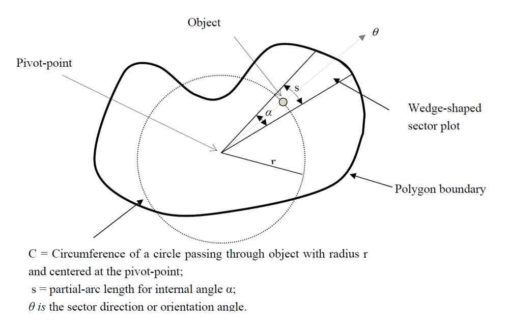
Sector sampling [1,2] was developed, but not confined to sampling objects in small complex polygons with lots of edge. Sector plots are “sector-shaped” fixed-angle plots with a randomly oriented central ray emanating from a vertex or “pivot-point” (see Figure 1). Uniquely, the pivot-point may be established subjectively [1,3]. In addition, there is no “edge effect” bias in sector plots as the selection probability for an object is the same anywhere in the sector plot, which is independent of proximity to a polygon edge [1].

Sector sampling is a new sampling technique in the forest and ecological literature and consequently there is little practical experience and few articles published. There have previously been papers in other disciplines using an angular section of a circle or ellipse such as: sampling the number of myelin or nerve fibers in the traverse sections on nerve fiber bundles [4,5,6]; sampling sunflower heads [7] and crowds of people [8]. In these instances, the statistical properties and techniques for calculating means and variances were not examined in any depth. It was not apparently noted that the pivot-point could be established subjectively rather than centrally, or that there was no object selection edge effect bias.

Initial sector sampling applications in forestry have included:

sampling young trees growing in and around groups of older leave trees, or “variable retention” [9,10] in forested settings [1,2];

estimating tree size in narrow, sinuous riparian strips [11]; and

sampling trees and small scattered woodlots outside the main forest [12,13].

The purpose of this paper is to review general sector sampling properties and current applications in the forest literature and to discuss and suggest additional potential ecological uses. Sector sampling may help extend sampling of some novel conditions with considerable edge that are not particularly well sampled using traditional approaches such as points or quadrats [14] or fixed area or variable probability plots or points [15].

2. Methodological Overview

 Figure 1 shows that sector sampling is based on fixed-angle, sector-shaped plots centered around an arbitrarily chosen central vertex or pivot-point. For any fixed internal plot angle, α, and a random direction, θ, the probability, p, of sampling an object in the plot is equal to the arc-length inside the sector plot, s, divided by the circumference, C or p = s/C = α/360°. For instance, if α = 36° then p = 10%. The inverse of the probability is the expansion factor (EF); sample values are increased by the EF to give estimates of population or polygon totals. Thus if α = 36°, EF = 10.

Figure 1. Schematic representation of sector sampling (Adapted from [2]).

Figure 1. Schematic representation of sector sampling (Adapted from [2]).

2.1. Plot Centers Can Be Established Subjectively

For an arc passing through an object, a random direction angle, θ, ensures an equal chance for any object to be selected along the circumference, C (Figure 1). The object selection probability, p = α/360° or s/C, depends only on the sector plot angle α and not the distance from the pivot-point, r. Hence, the pivot-point can be located anywhere inside or outside the polygon and the object selection probability is always α/360° [1,2,3]. Under these conditions the pivot-point can be located at the convenience of the sampler. This remarkable property is unique to sector sampling and has a great deal of practical utility such as ensuring a viewpoint which avoids errors in counting objects, and is easy to locate and document. In addition there are advantages of safety, and efficiency, for instance obviating rock outcrops, scree slopes, bear dens, wasp’s nests or swamps at the plot center.

2.2. No Edge Effect on Object Selection Probability

If fixed or variable area plots are established around an object and straddle a polygon or sample area boundary then the object selection probability is altered [16,17,18], see [18] (p. 624). Part of the plot centered on the object lies outside the polygon so that the selection probability is underestimated, as are estimates of totals associated with the object such as plant biomass or bird nests. A direct correction is to weight each object by (area plot)/(area plot inside the polygon), see [18] (p. 627), but this is not easy to do in the field as each object must be visited and distance to the edge measured. Sector plots have no such edge effect: the probability of tree selection has nothing to do with tree location, plot location, or polygon shape [1]. The sector plot extends up to the polygon boundary with no effect on tree selection probability. This is a distinct advantage of sector plots and avoids complex adjustments and bias. In small areas with lots of edge to area this is a particularly useful property.

2.3. Expansion Factors Used to Obtain Polygon Means and Totals

The probability of object selection under sector samplingis fixed for any given angle α; hence, polygon or sample unit totals, per tree values or numbers of items may be unbiasedly calculated using simple random sampling (SRS) formulae [1] by multiplying sector plot totals by the expansion factor, 360°/α. Next, several other random or systematic sectors may be located at the same pivot-point and SRS formulae used to calculate totals and associated variances across the sectors [1]. If polygon area is known then units may be placed on an estimated per unit area basis; polygon totals and any associated variances may simply be calculated by dividing by polygon area or area squared, respectively.

2.4. Ratio Estimates for Unit Area Values

If actual sector area is known, then per unit area values can be calculated directly. For instance basal area (BA) may be calculated for each sector by summing each tree BA and dividing that total by the sector area to give basal area per unit area. In this case, the appropriate estimate is a ratio-of-means (ROM) estimator for means and variances (BA/area): larger sectors account for larger areas and are weighted more [2]. This is analogous to a Horvitz-Thompson [19] estimator with sector areas as the weights. Thus, if one sector has twice the area of another in the same sample, then the first carries twice the weight when combining the sectors. If the polygon is regular in shape and the pivot-point is in the center then essentially all sectors will have equal areas so SRS formulae for means or variances might be used as a reasonable approximation. If the polygon is highly irregular or the pivot-point is off-center in a regular polygon then a ROM estimation variance formulae should be used,see [20] (p. 153). Smith et al. [2] found that the ROM variance could be underestimated by up to 40% for small sample size (n

2.5. Random Angles Versus Random Points for Selecting Direction Angle

ROM formulae may be used when direction angles are established randomly (“random angle” method). It appears to be generally more efficient, however, to base sector direction angle on “random points” achieved by establishing sector direction through points randomly located in the polygon. This ensures that objects in larger parts of the polygon get sampled in proportion to area; the data are already “weighted” correctly so that SRS formulae for means and variances may be used rather than ROM formulae [2]. Random point selection is a form of importance sample, choosing larger areas of the polygon more frequently.

2.6. Systematic Sectors

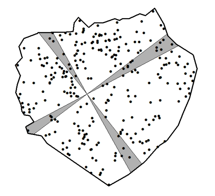
A systematic sample of sectors reduces the variability between sectors by averaging out the area differences (Figure 2). This is an antithetic-variate method of variance reduction: for off-center pivot-points or pivot-points inside an irregular polygon a large sector will generally be balanced off by a small sector if they are 180° apart, thus reducing variability by giving a larger negative covariance. This technique makes the random angle method similarly efficient to the random point method.

Figure 2. A 10% systematic sample of objects in a polygon using four orthogonal 9° sectors. Objects (trees) shown as black dots. Based on [2].

Figure 2. A 10% systematic sample of objects in a polygon using four orthogonal 9° sectors. Objects (trees) shown as black dots. Based on [2].

2.7. Sub-Sampling Sectors

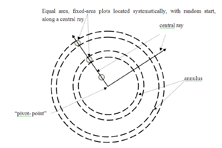
The sector area increases proportionally with distance from the pivot-point, with a consequent increase in the number of objects to be counted. To reduce field work the sector can be divided into two or more sectors along the central axis and one selected at random. The trees would then need to be weighted appropriately (e.g., weight is 2 if sector is bisected into two). If a smaller subsample needs to be made then a systematic selection of an annulus bounded by the sector plot edges may be made at fixed or random points along the sector central axis. The probability of object selection is then equal to [α/360° ° (length of the partial annulus along sector central ray)/(sub-sample interval)].

3. New Applications

3.1. Subsampling Using Fixed Area Plots

A sector plot sub-sampling system comprising small fixed area plots established along the central ray may also be used (see Figure 3). In this case, provided the plot does not overlap the polygon boundary (here represented as the larger circle) or the pivot-point, then the probability of selection for an object in the plot is equal to (plot area)/(annulus area) which is inversely proportional to distance along the sector central ray from pivot-point to object center:

$$\mathit{EF}=\frac{(\mathit{R}+\mathit{r}){}^2-(\mathit{R}-\mathit{r}){}^{\mathrm{2}}}{{\mathit{r}}^{\mathrm{2}}}=\frac{4\mathit{R}}{\mathit{r}}\propto \mathit{R}$$

where EFis tree or plot expansion factor (the inverse of selection probability) which is the area of an annulus that is represented by the plot, R is distance from pivot-point to plot center and r is the radius of the plot.

The probability of object selection is more complex at both extremities of the central ray; for a plot centered at the pivot-point the selection probability is bounded at p = 1. For a small plot overlapping the polygon boundary edge this bias [16,18], see [18] (p. 621), must be accounted for in the strict sense, but our simulations indicate that the effect is negligible for small plots. There is an exact edge effect solution based on the overlap of each object for a given plot size [16], discussed above. In addition, there are also several practical ways to eliminate the edge effect along the borders. These include the “walkthrough” method of Ducey et al. [21], and the “toss-back” method of Iles, see [18] (p. 645). Accounting for selection probabilities is only of practical importance if the polygon area is small with large edge to area amounts. Nevertheless, the ease of establishment of fixed area plots is traded off for greater computational complexity.

Figure 3. Sub-sampling sectors using fixed area plots.

Figure 3. Sub-sampling sectors using fixed area plots.

Figure 4. Sampling down objects using sector plots: a systemic location of two partial-arcs with a random start is shown; α is the internal sector angle.

Figure 4. Sampling down objects using sector plots: a systemic location of two partial-arcs with a random start is shown; α is the internal sector angle.

3.2. Using Sector Plot Arcs to Measure Down and Linear Objects

The presence of down trees or horizontal linear objects such as dead woody debris may be sampled using sector plots. Traditionally, linear transects have been used [18,22,23]. Sector plots may also be used with the transect based on the sector “partial-arc”. An example of using sector sampling to count the number of down or linear objects in a polygon is shown (Figure 4). In this example a systematic arrangement of partial-arcs, s, with a random start is used. Then the number of down or linear objects whose axis crosses the partial-arcs is calculated as:

Number of down or linear objects per hectare equation 2

$$=\frac{\mathrm{\pi }}{2\mathit{L}}\sum _{\mathit{i}}^{\mathit{n}}\left(\frac{1.0}{{\mathit{l}}_{\mathit{i}}}\right)\left(\frac{{360}^{\mathit{o}}}{\mathrm{\alpha }}\right)\times 10,000$$

where li = horizontal length of the ith object (in metres), i = 1, …, n or the number of objects crossing the partial-arc, L is the horizontal length (in metres) of the partial-arc and 360°/α is the sector expansion factor, with α in degrees. In order to “count” the objects it is necessary to measure their lengths. The partial-arcs sample the down objects proportional to horizontal length: hence object count is weighted by 1.0/li. The factor π/2 is the correction under the assumption of a random orientation of object axis [24] relative to the partial-arc. Finally, 10,000 converts from objects per m2 to per hectare. The simple average of equation (1) for other systematic partial-arcs per sector gives an estimate of total number of pieces per hectare in the polygon. Under traditional sampling using linear transects, means and variances are weighted by transect length. However, under sector sampling the data are “automatically” weighted by transect length. The length of each partial-arc is proportional to the distance from the pivot-point, thus SRS sampling formulas can be used for means or variances without any special weighting. Note that equation (1) is identical to standard transect sampling formulas using straight transects except for the sector expansion factor, 360°/α. The partial-arcs are not randomly oriented and, therefore, are not always theoretically unbiased; but it is our opinion that this effect would be minimal in most practical situations. To avoid this just measure the crossing angle of the object.

3.3. Measuring Length of Linear Features

It is also possible to use sector sample transects to help estimate the total length of game trails, roads, hedgerows, streams or other linear features, see [18] (p. 409). Simply count the number of times the features are traversed as in standard transect sampling and expand using the sector expansion factor:

Horizontal object or feature length in meters per hectare equation 3

$$=\frac{\mathrm{\pi }}{2}\left(\frac{\mathrm{count}}{\mathit{L}}\right)\left(\frac{{360}^o}{\mathrm{\alpha }}\right)\times 10,000$$

This same general approach may be extended to down woody debris volume by calculating the cross sectional area of debris crossing the partial-arc and “spreading-out” along the partial sector length, s, to get the average “depth” of wood along s. This number can then be multiplied by 360°/α to get volume along the whole arc.

3.4. Sampling Framework for Monitoring “Variable Retention”

In several parts of the world, for instance, in some forested areas of Tasmania [25,26], some areas of the Canadian Pacific Northwest [10], the U.S. Pacific Northwest [27,28], and the South American Patagonia [29,30], variable retention silviculture [10,31,32] is being used to leave behind groups of aggregated or dispersed forest retention. Sector sampling was originally designed to sample variable retention tree responses in experimental settings. Traditional data collection techniques, such as fixed area plots or transects, were not designed to be applied efficiently to these new and unique forest structures.

Figure 5 shows an example of a two-stage sector sampling layout in large scale (100 ha) experimental variable retention areas set up on public land during 2000–2010 in coastal British Columbia [32]. The intent was to examine the growth of regenerating trees in proximity to retained taller groups of trees. There were 3 randomly allocated treatments leaving 10%, 20% and 30% of initial area in small aggregated retention groups of trees (each 0.2 ha to 0.4 ha in size), an unharvested (“control”) and clearcut area.

The procedure was a two-stage one. In the first stage smaller sub-sample areas were delineated that tessellated the area. Here, areas from one up to two hectares were marked using roads and permanent features in the clearcut and unharvested control. This is shown fully for the clearcut, 10% and 20% group retention areas and partially for the 30% retention area (Figure 5). The simple stratification along visible boundaries that are easy to find on the land base is a nice advantage of the system. It is not obvious, perhaps, but the areas of these strata do not affect the probability of trees being sampled, as probability of tree selection depends only on the sector angle, and the data are easy to combine afterwards, see [1] (p. 151).

 Five sub-sample areas were selected at random in the clearcut and control areas and full sector plots with a 36° internal angle located at plot center using a random direction angle and sectors extending to the sub-sample boundary (Figure 5).

In the harvested, 10%, 20% and 30% variable retention experiment treatments the aggregated retention patches and surrounding harvested areas were demarcated using roads or other permanent survey features and three patches chosen randomly in each treatment. In the approximate center of each selected patch per treatment four orthogonal systematic sectors, each 9° and summing to 36° (a 10% sample), were established with a random orientation and extended to the sub-sample boundary.

The objective was to monitor the development of the retained, regenerating and planted trees in N, S, E and W directions. In the clearcut and unharvested control area this azimuthal hypothesis was not tested so the four sectors were collapsed into one. The plots are easy to install in the field: simply establish the central axis using GPS, laser or by lining up stations and use radial or distances offsets to locate sector sides. We have found that using a 10% sample (36°) is a useful operational starting point though more work could be done to develop the most efficient sector angle for a given set of conditions.

3.5. Additional Potential Applications

 There are numerous other sampling applications that might be envisaged—as an example: the inventory of fauna and flora in small areas, copses or hedgerows. The sector plot could be positioned in the center of a clearcut or field and used to randomly sample forest edges or boundaries for windthrow or hedges for nesting birds. In the ocean, corals may be readily sampled, as would small areas around moored boats. Birds or other animals could be counted using a fixed angle gauge with random orientation along linear strips or on lake surfaces. Distance along the sector might also be used to examine environmental gradients. Items on the ground such as nests or animal tracks and trails could also be measured. For fast moving objects crossing the sector plots photographs or videos might be taken and enumerated at a later date. Another variant is to use sector sampling to sub-sample point distance samples [33] in cases where there are many or difficult objects to count.

Figure 5. Schematic example of sector plot layout in an aggregated retention forested setting experimental area. The control area is unharvested, the clearcut area is harvested and the 10%, 20% and 30% groups have small groups of trees (approx. 0.3 ha in size) surrounded by harvested areas. “10% Groups” refers to 10% of the treatment area covered in retained groups, etc.

Figure 5. Schematic example of sector plot layout in an aggregated retention forested setting experimental area. The control area is unharvested, the clearcut area is harvested and the 10%, 20% and 30% groups have small groups of trees (approx. 0.3 ha in size) surrounded by harvested areas. “10% Groups” refers to 10% of the treatment area covered in retained groups, etc.

4. Further Comments

Sector plots were originally designed to sample objects in small polygons with extensive edges. There is no edge overlap bias as there is in fixed or variable plots that select objects which straddle a polygon boundary. Corona et al. [12] showed this to be a marked sampling efficiency advantage when selecting sector plots compared to fixed area plots in a simulation sample of small woodlots. Tongson et al. [13] also showed great practical advantage to sampling scattered trees outside the main forest survey area. In variable retention settings, avoiding edge bias issues neatly sidesteps considerable analysis complexity. A further advantage is in being able to establish the sector plot pivot-point subjectively.

Sector plots may be conveniently sub-sampled by splitting longitudinally in a successive fashion along a central axis and/or latitudinally into annuli. Small fixed area plots may be more easily set up in the field; for instance in sub-sampling dense brush or regeneration, but edge effect biases require correction.

Down woody debris or other linear features may conveniently be sampled using the partial-arcs of sector plots. In this situation the advantage of subjective plot location is of significant practical convenience for plot establishment such as in a high windthrow area with many down trees to count and measure. If a part of the object designated as defining the object to be “in” the polygon is within the sector there is no edge effect problem for the number of objects; that might be the midpoint, or the largest end of the object, for instance.

Sector sampling is a new sampling technique so that few applications have been made or documented, yet many applications can be envisaged. Potential new applications might include sampling boundaries such as hedgerows for bird nests or species composition or counts of objects at forest edges such as windthrow trees. Small islands of vegetation or grouped structures such as ponds, swamps, rocky outcrops, lakes, sea corals, shell fish beds or ocean vents could also be effectively enumerated.

5. Conclusions

Sector plots are a new sampling methodology particularly suited to sampling objects in small areas and/or situations with lots of edge. The advantages are that the plot center can be located subjectively and there are no edge effects biasing object selection near the boundaries of sampling units. If large numbers of objects are being sampled then the sector plots may be readily sub-sampled. Statistics are also easy to calculate. Plot establishment is simple and straightforward. The plot centre can be established to avoid inconvenient locations and to improve visibility and monumentation. In addition, count items at ground level such as leaves, branches, fungal mycelia or rabbit burrows may also be easily enumerated. Sector sampling may have a place in monitoring and experimental verification of new and novel and complex habitats especially those with excessive edges.

References

- Smith, N.J.; Iles, K. A new type of sample plot that is particularly useful for sampling small clusters of objects. For. Sci. 2006, 52, 148–154. [Google Scholar]
- Raynor, K.; Iles, K.; Smith, N.J. Investigation of some sector sampling statistical properties. For. Sci. 2008, 54, 67–76. [Google Scholar]
- Lynch, T.B. Variance reduction for sector sampling. For. Sci. 2006, 52, 251–261. [Google Scholar]
- Donovan, A. The nerve fibre composition of the cat optic nerve. J. Anatomy 1967, 101, 1–11. [Google Scholar]
- Gerritsen, G.C.; Swartzman, J.; Fix, J.D.; Davis, D.E.; Diani, A.R. Acta Neuropathol. 1981, 53, 293–298. [CrossRef] [PubMed]
- Sharma, A.K.; Mayhew, T.M. Sampling schemes or estimating nerve fibre size. II: Methods for unifasicular nerve trunks. J. Anatomy 1984, 139, 59–66. [Google Scholar]
- Robinson, R.G. Maturation of sunflower and sector sampling of heads to monitor maturation. Field Crop. Res. 1983, 7, 31–39. [Google Scholar] [CrossRef]
- MacGillivray, L.; Meyer, K.; Seidler, J. Collecting data on crowds and rallies: A new method of stationary sampling. Soc. Forces 1976, 55, 507–519. [Google Scholar]
- Tappeiner, J.C.; Thornburgh, D.A.; Berg, D.R.; Franklin, J.F. Alternative silvicultural approaches to timber harvesting: Variable retention harvest systems. In Creating a Forestry for the 21st Century: The Science of Ecosystem Management; Kohn, K.A., Franklin, Ed.; 1997; Island Press: Washington, DC, USA. [Google Scholar]
- Dunsworth, G.B.; Bunnell, F.L. Forest Biodiversity: Learning How to Sustain Biodiversity in Managed Forests,1st ed.; 2009; University of British Columbia Press: Vancouver, BC, Canada. [Google Scholar]
- Anderson, P.D.; Temesgen, H.; Marquardt, T. Accuracy and suitability of selected sampling methods within conifer dominated riparian zones. For. Ecol. Manage. 2010, 30, 313–320. [Google Scholar]
- Franceschi, S.; Fattorini, L.; Corona, P. Two-stage sector sampling for estimating small woodlot attributes. Can. J. For. Res. 2011, 41, 1819–1826. [Google Scholar] [CrossRef]
- Prasomsin, P.; Duangsathaporn, K.; Tongson, P.K. Yield assessment of tree resources outside the forest using sector sampling: A case study of a public park, Bangkok Metropolis, Thailand. Kasetsart J. (Nat. Sci.) 2011, 45, 396–403. [Google Scholar]
- Grieg-Smith, P. Quantitative Plant Ecology (Studies in Ecology),3rd ed.; 1983; University of California Press: Berkeley and Los Angeles, CA, USA. [Google Scholar]
- Ramirez-Maldonado, H.; Ernst, R.; Schreuder, H.T. Statistical Techniques for Sampling and Monitoring Natural Resources; 2004; General Technical Report RMRS-GTR-126; USDA Forest Service,Rocky Mountain Research Station: Fort Collins, FL, USA. [Google Scholar]
- Scott, C.T.; Gregoire, T.G. Sampling at the stand boundary: A comparison of the statistical performance among eight methods. In. In Proceedings of the XIX IUFRO World CongressMontreal, QC, Canada, 5–11 August 1990; Lowe, J.J., Bonnor, G.M., Burkhart, H.E., Eds.; Virginia Polytechnic Institute State University: Blacksburg,VA,USA,1990;
- Scott, C.T.; Gregoire, T.G. Altered selection probabilities caused by avoiding the edge in field surveys. J. Agric. Biol. Envir. Stat. 2003, 8, 36–47. [Google Scholar] [CrossRef]
- Iles, K. A Sampler of Inventory Topics,1st ed.; 2003; Kim Iles : Nanaimo, BC, Canada. [Google Scholar]
- Thompson, D.J.; Horvitz, D.G. A generalization of sampling without replacement from a finite universe. J. Amer. Stat. Assoc. 1952, 47, 663–685. [Google Scholar]
- Cochran, W. Sampling Techniques,3rd ed.; 1977; John Wiley and Sons: New York, NY, USA. [Google Scholar]
- Valentine, H.T.; Gove, J.H.; Ducey, M.J. A walkthrough solution to the boundary overlap problem. For. Sci. 2004, 50, 427–435. [Google Scholar]
- Olsen, P.F.; Warren, W.G. A line intersect technique for assessing logging waste. For. Sci. 1964, 10, 267–276. [Google Scholar]
- Van Wagner, C.E. The line intersect method in forest fuel sampling. For. Sci. 1968, 14, 20–26. [Google Scholar]
- Matern, B. On the geometry of the cross-section of a stem. Meddelanden Fran Statens Skogsforskningsinstitut 1956, NR 11, 1–28. [Google Scholar]
- Bashford, D.; Bonham, K.J.; Forster, L.; Grove, S.J.; Baker, S.C. Short-term responses of ground-active beetles to alternative silvicultural systems in the Warra Silvicultural Systems Trial, Tasmania, Australia. For. Ecol. Manage. 2009, 258, 444–459. [Google Scholar] [CrossRef]
- Grove, S.J.; Neyland, M.; Baker, S.C. Using aggregated retention to maintain and restore mature forest values in managed forest landscapes. Project summary. Ecol. Manage. Restor. 2010, 11, 82. [Google Scholar]
- Peterson, C.E.; Halpern, C.H.; Aubrey, K.B. Variable-retention harvests in the Pacific Northwest: A review of short-term findings from the DEMO study. For. Ecol. Manage. 2009, 258, 398–408. [Google Scholar] [CrossRef]
- Anderson, P.D.; Peterson, C.E. Large-scale interdisciplinary experiments inform current and future forestry management options in the U.S. Pacific Northwest. For. Ecol. Manage. 2009, 258, 409–418. [Google Scholar] [CrossRef]
- Cellini, J.M.; Gallo, E.; Pastura, G.M.; Lencinasa, M.V. Alternative silvicultural practices with variable retention improve bird conservation in managed South Patagonian forests. For. Ecol. Manage. 2009, 258, 472–480. [Google Scholar] [CrossRef]
- Estebana, R.S.; Peric, P.L.; Cellinib, J.M.; Lencinasa, M.V.; Pastura, G.M. Timber management with variable retention in Nothofagus pumilio forests of Southern Patagonia. For. Ecol. Manage. 2009, 258, 436–443. [Google Scholar] [CrossRef]
- Beese, W.J.; Mitchell, S.J. The retention system: Reconciling variable retention with the principles of silvicultural systems. For. Chron. 2002, 78, 397–403. [Google Scholar]
- Smith, N.J.; Dunsworth, G.B.; Beese, W.J. Variable retention adaptive management experiments: Testing new approaches for managing British Columbia’s coastal forests. In Balancing Ecosystem Values: Innovative Experiments for Sustainable Forestry; Maguire Peterson, C.E., Ed.; 2005; pp. 436–443. General Technical Report PNW-GTR-635; USDA Forest Service,PNW Research Station: Portland, OR, USA. [Google Scholar]
- Strindberg, S.; Borchers, D.L.; Laake, J.L.; Anderson, D.A.; Burnham, K.P.; Buckland, S.T.; Thomas, L. Encyclopedia of Environmetrics; El-Shaarawi, A.H., Piergorsch, Ed.; 2002; John Wiley and Sons: Chichester, UK. [Google Scholar]
© 2012 by the authors; licensee MDPI, Basel, Switzerland. This article is an open-access article distributed under the terms and conditions of the Creative Commons Attribution license (http://creativecommons.org/licenses/by/3.0/).
Share and Cite
MDPI and ACS Style
Smith, N.J.; Iles, K. Sector Sampling—Synthesis and Applications. Forests 2012, 3, 114-126. https://doi.org/10.3390/f3010114
AMA Style
Smith NJ, Iles K. Sector Sampling—Synthesis and Applications. Forests. 2012; 3(1):114-126. https://doi.org/10.3390/f3010114
Chicago/Turabian StyleSmith, Nicholas J., and Kim Iles. 2012. "Sector Sampling—Synthesis and Applications" Forests 3, no. 1: 114-126. https://doi.org/10.3390/f3010114