Greenhouse Gas Balance of Native Forests in New South Wales, Australia

Abstract

To quantify the climate change impacts of forestry and forest management options, we must consider the entire forestry system: the carbon dynamics of the forest, the life cycle of harvested wood products, and the substitution benefit of using biomass and wood products compared to more greenhouse gas intensive options. This paper presents modelled estimates of the greenhouse gas balance of two key native forest areas managed for production in New South Wales for a period of 200 years, and compares it to the option of managing for conservation only. These two case studies show that forests managed for production provide the greatest ongoing greenhouse gas benefits, with long-term carbon storage in products, and product substitution benefits critical to the outcome. Thus native forests could play a significant part in climate change mitigation, particularly when sustainably managed for production of wood and non-wood products including biomass for bioenergy. The potential role of production forestry in mitigating climate change, though substantial, has been largely overlooked in recent Australian climate change policy.

1. Introduction

Australia has approximately 4% of the world’s forests, comprising 147.4 million hectares (Mha) of native forest and 2.0 Mha of forestry plantations, covering about 19% of the continent [1]. Approximately 9.4 Mha of publicly owned native forests are managed for multiple use (including timber production) in Australia [1]. The National Forest Policy Statement set a course for major change in Australia’s native forest industry, with the objectives of: establishing a comprehensive, adequate and representative forest reserve system; implementing ecologically sustainable forest management practices; and establishing an internationally competitive, value-added industry [2]. As a consequence in New South Wales (NSW), the area of public native forests managed for multiple use was reduced from 2.6 Mha in 1990 [3] to 1.3 Mha by 2008 [4] through conversion to conservation reserves.

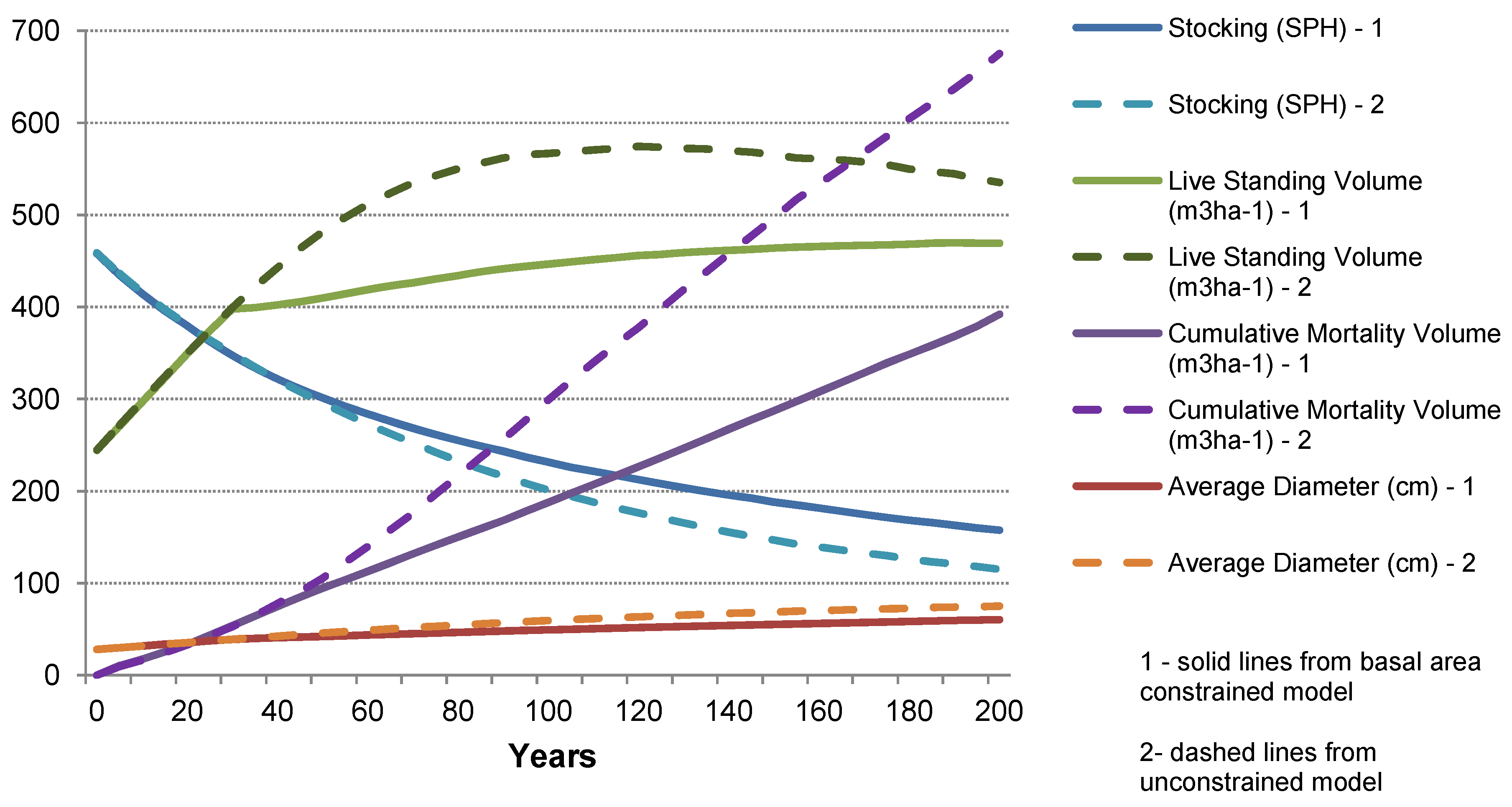
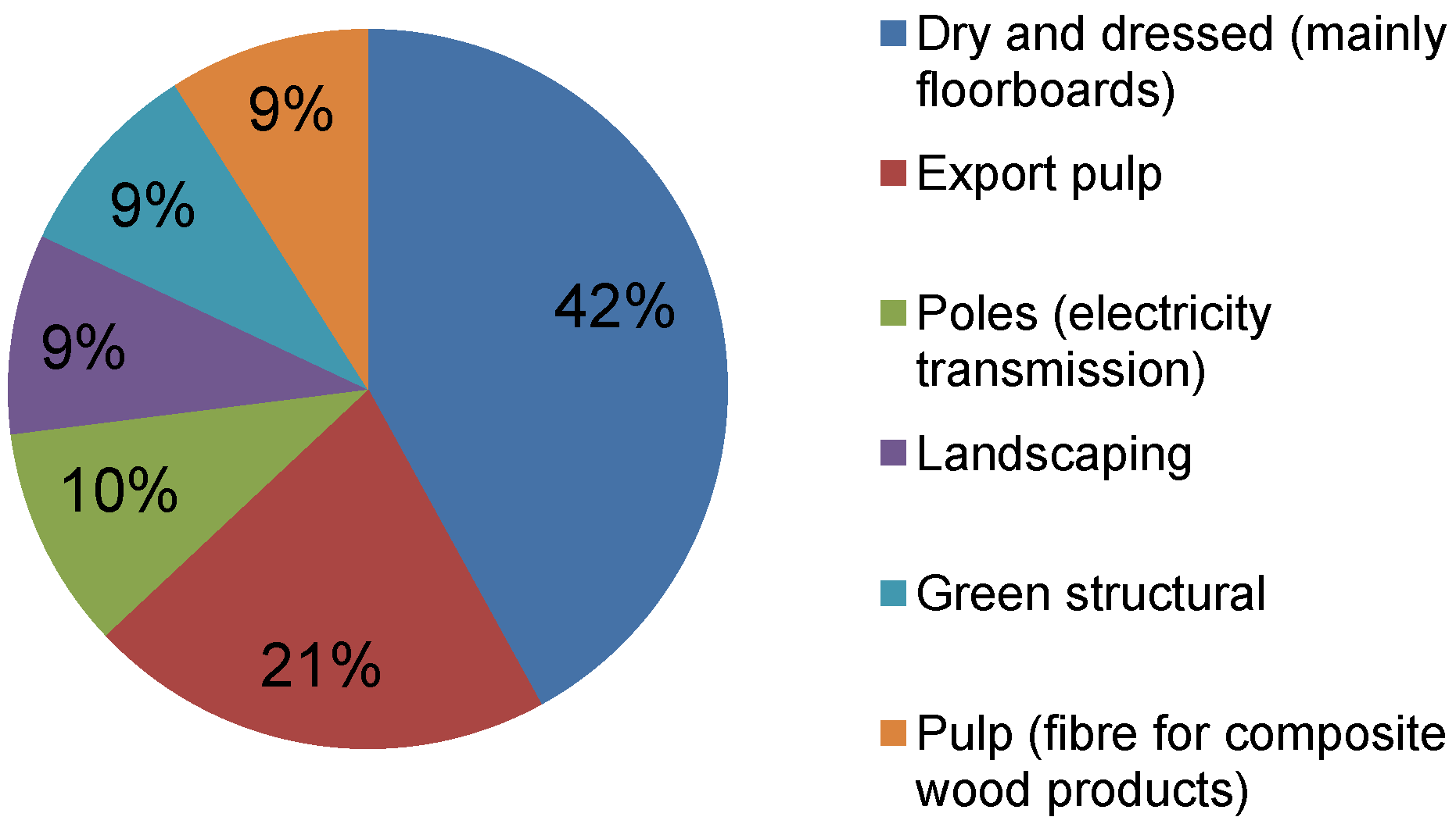
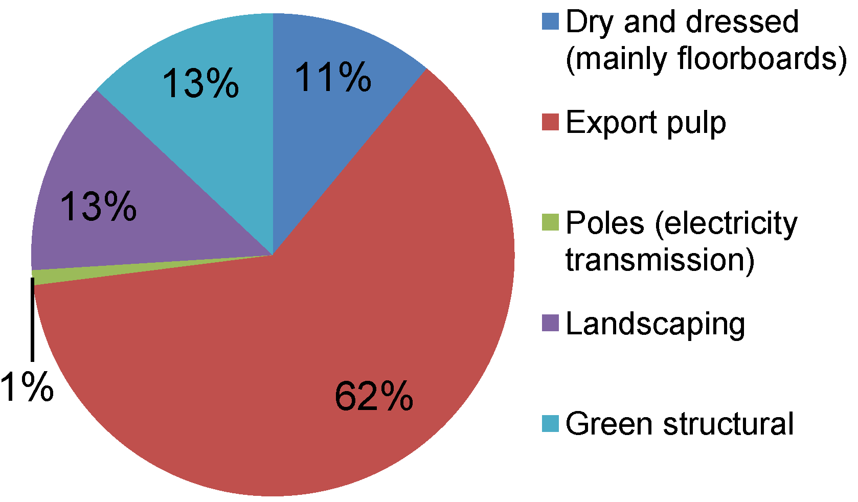
When forests are harvested in Australia the amount of biomass removed for processing into wood products varies between 45% and 65% for different forest types, ages and locations [5]. The proportion of extracted logs in different product classes varies substantially between tree species. The proportion of highly value-added hardwood products such as floorboards, decking and furniture has increased from 29% in 1995/1996 to 62% in 2008/2009 [4].

At the end of their service life, the vast majority of harvested wood products (HWPs) in Australia are deposited in landfill. Although some HWPs may be recycled at least once, eventually a high proportion of recycled HWPs will also end up in landfills. The majority of the C in HWPs deposited in landfill remains undecomposed [6]. Carbon in HWPs in landfill is quantified from estimates of waste composition and volume, and assumed decay rates [7]. Decomposition of organic materials in landfills results in the generation of greenhouse gas (GHG), mainly carbon dioxide and methane in approximately equal proportions. Emissions typically occur over a period of approximately 30 years after the waste has been deposited. The decomposition factors used are critical to the calculation of GHG emissions from landfills, as methane is a GHG 21–25 times more powerful than carbon dioxide. In the IPCC Guidelines [7] it is currently assumed that 50% of the C in HWPs in landfill is released as a result of decomposition. However, recent field-based research (e.g., [6]), and a recently published experimental study in the USA [8], have demonstrated that HWPs in landfill represent a long term C store, with minimal or no decomposition taking place.

Besides storing C sequestered during forest growth, HWPs can provide additional GHG mitigation benefits through the substitution for other more energy and GHG-intensive materials such as steel, aluminium, plastic and concrete [9]. Research from around the world has shown that the life-cycle GHG impact of HWPs is significantly lower than that of competing, non-renewable products (e.g., Australia and New Zealand [10,11,12,13]; Europe [14,15]; US [16,17]). A meta-analysis of twenty European and North-American studies found an average reduction of two tonnes of C for each tonne of C in HWPs substituted for non-wood products [14].

Similar benefits through fossil fuel displacement may be achieved by the use of harvest residues for bioenergy production. Forest residues comprise the bole of the tree remaining after the commercial logs are removed, the crown, bark, limbs, and entire trees that are not marketable due to size, bends and twists or internal defect such as rot. On the north coast of NSW over 600,000 tonnes per annum of sawlogs and other products are sold each year, with the remaining 300,000+ tonnes of forest residue left on the ground. In practice, harvest residues often create a fire risk and usual practice is to burn them post-harvest. This adds operational cost and risk and results in GHG emissions. If not burnt, these residues are assumed to decay over a 10–20 year time frame releasing their C back into the atmosphere [18]. In Australia it is a requirement by 2020 that 20% of the electricity generation is produced from renewable sources [19]. This will represent a substantial increase from current levels (8% of the electricity is currently generated from renewable sources [20]), representing a significant opportunity for increased biomass use.

Greenhouse emissions due to fire events are an important component of the global carbon cycle [21]. Fire is an intrinsic aspect of the ecology and management of SE Australian forests and woodlands [21]. Prescribed burning is the principal means of managing fuel levels in Australian forests, with the aim to reduce wildfire risk [22]. The frequency and severity of wildfire events vary significantly according to the forest type. There is circumstantial evidence that fuel reduction programs have reduced the impact of wildfires on forest land: in NSW wildfires have been low in State Forests, but widespread on other land tenures [23].

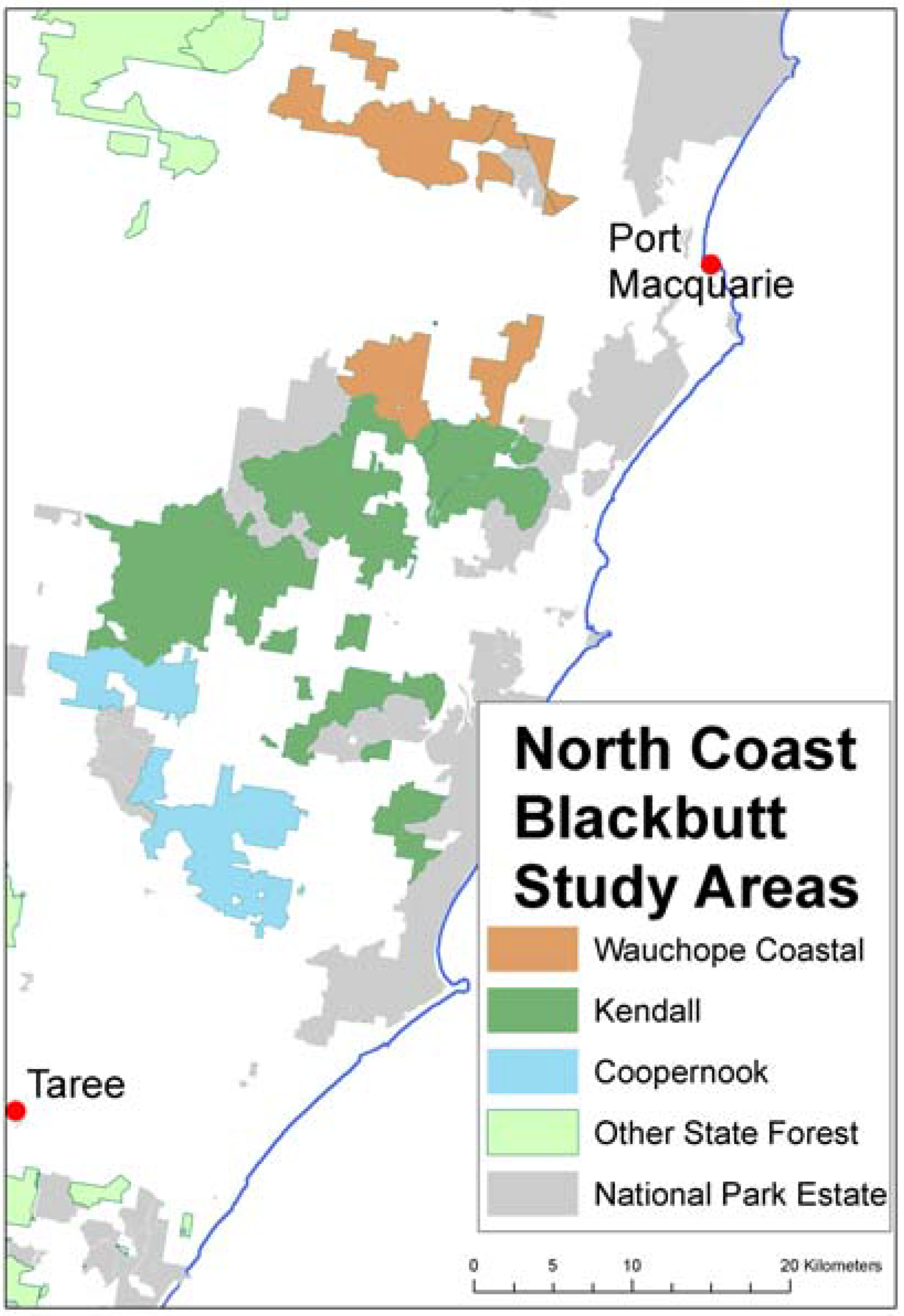
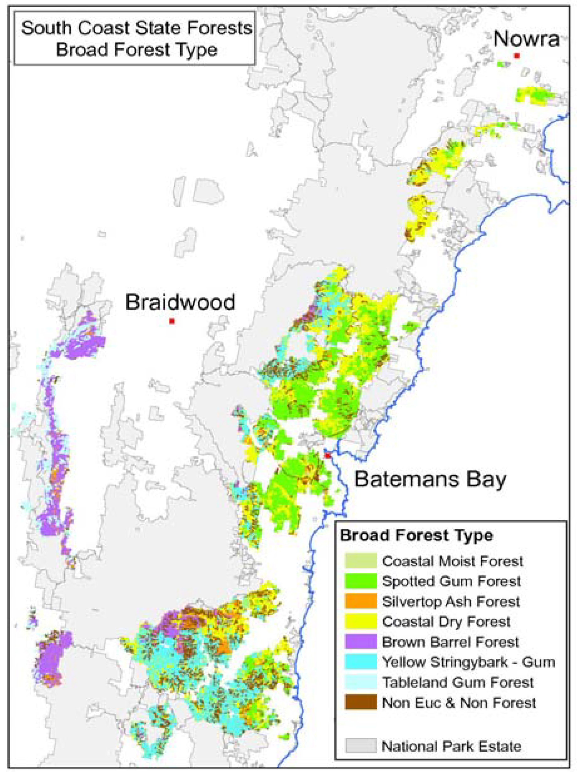
The key objective of this paper is to estimate the impact on net GHG emissions to the atmosphere of converting multiple use production forests into forests managed for conservation purposes only in NSW. In order to understand the full contribution that forests managed for wood products can deliver in reducing GHG emissions, we estimate the impact of different harvest scenarios on carbon levels in forest and wood products over time, for the two case study regions. In addition we assess the potential emissions offset due to product substitution and displacement of fossil energy emissions.

2. Methods and Background Information

The GHG impact of alternative forests management is presented for two case studies, based on NSW native forests from the north coast (NC) and south coast (SC) areas. All relevant processes within the forest and offsite are considered in the GHG balance of forests managed for:

• (1) multiple use (“production”)—sustainably managed for the production of wood products and fibre and maintenance of natural resource management values; or
• (2) conservation only (“conservation”)—managed as part of the nature conservation reserve system with no harvesting.

2.1. Scope of the Analyses

Changes in carbon stock over time of both forests and in HWPs were considered (expressed as tonnes of carbon per average hectare of forests). The simulation was run over a period of 200 years. As the aim of the study was to compare management options, the “production” and “conservation” management scenarios were modelled on the same sites and thus represent exactly the same forest productivity. We predict that if harvest is eliminated in the areas of our case studies that there will be one or a combination of two outcomes:

• (1) Harvest will remain constant elsewhere and HWPs consumption will decrease resulting in an change in GHG emissions associated with production and use of non-wood products; or
• (2) Harvest will increase elsewhere to maintain consumption of HWPs; however these HWPs are likely to be imported, which may affect GHG emissions from forest carbon stock changes elsewhere.

Only the first outcome (change in non-wood products consumption) is included in the modelling—however the potential implications for forest carbon stocks in countries exporting native hardwood to Australia is explored further in the “Discussion” section.

The forest “production” scenario takes into account:

• • Above-ground forest C—C removed from or added to the atmosphere by the growing forest (expressed as the change in long term average C stock);
• • C storage in harvest residues (above and below-ground); this is included in the “above-ground forest C” component above;
• • C storage in HWPs in use and in landfill;
• • GHG emissions due to the establishment and management of forests, harvesting and log transport;
• • GHG emissions due to manufacture of products and transport to customer;
• • GHG emissions due to disposal of products;
• • GHG emissions due to transport of harvest residues to the power station.

The forest “conservation” scenario takes into account:

• • Above-ground forest C—C removed from or added to the atmosphere by the growing forest (expressed as the change in long term average C stock);
• • GHG emissions for non-wood products manufacture and use;
• • GHG emissions from fossil energy (GHG emissions that would happen due to the use of coal in electricity generation if harvest residues were not used for energy).

The GHG emissions for non-wood products manufacture and use and from fossil energy were assigned to the “conservation” scenario to more accurately reflect fluxes over the simulation period.

Based on the parameters described above, the substitution effect can be described as:

• • Substitution_HWP: The difference between GHG emissions to make and use non-wood product and GHG emissions to make and use equivalent HWPs;
• • Substitution_RES: fossil-fuel GHG emissions avoided by using a proportion of harvest residues for bioenergy generation;
• • Substitution_EOL: fossil-fuel GHG emissions avoided by combusting HWPs for energy at the end of their service life.

A more detailed description of the different forms of substitution benefits is included in sections 2.9–2.11.

Forest soil C was assumed to be at steady state over the 200 years. Native forest harvesting operations carried out sustainably under existing agreed protocols typically produce only a slight change, if any, to total soil C levels [13,24].

GHG emissions due to wildfire and prescribed burning (non-CO₂) were not directly included in the analyses, due to the lack of site-specific data. Instead the potential impact of including those emissions on the net GHG balance of the case study forests, using best available published references, were discussed. We also discuss but do not explicitly include the effect of incorporating C in coarse woody debris (CWD) in the analysis, and the effect that a decrease in harvest within the systems could have, through market forces, on harvest and forest carbon in other domestic or foreign forests.

2.2. Forest Types

For the NC forests case study, three forest zones (Coopernook, Kendall and Wauchope Coastal) dominated by mature regrowth blackbutt (Eucalyptus pilularis) established from harvest and timber stand improvement in the 1950’s and 1960’s were selected (Figure 1). Blackbutt is the most commercially important species in NSW [25]. The SC case study covered seven forest yield associations (Coastal Moist Forest, Spotted Gum, Silvertop Ash, Coastal Dry Forest, Brown Barrel, Yellow Stringybark-Gum and Tableland Gum) containing a variety of dominant species (Figure 2).

Figure 1. North Coast case study areas.

Figure 1. North Coast case study areas.

Figure 2. South Coast case study areas.

Figure 2. South Coast case study areas.

The study areas are representative of the range of “average” site productivity forests, silviculture and product mix across native forests in eastern Australia. The selected forests have generally higher productivity than the inland mixed hardwood/cypress dominated forests of NSW, Victoria and Queensland, but lower than the productive “ash” types in Victoria and Tasmania. The pulpwood/sawlog ratio is high for SC forests but low for NC forests—the majority of other Australian native forests fall somewhere in between. Similarly, silvicultural practices in most other Australian native forests fall somewhere in between the SC (moderate intensity) and the NC (relatively intensive) forests (clearfall “ash” forest silviculture is more intensive) [25].

Details of the NC and SC stands are included in Table 1 below. The NC forest stands were similar in structure (based on average plot data for the three forest zones) and the basal area (BA) ranged from 28.2 to 29.5 m² ha⁻¹. The SC forest zones covered a broader range of forest type and stand conditions and BAs ranged from 25.3 to 44 m² ha⁻¹ (Table 1). The total area for the NC and SC forest zones was 18,132 ha and 99,943 ha, respectively. Combined the two areas account for approximately 12% of the native forest state available for harvest in NSW and 25% of the volume of sawlogs produced in NSW [4]. These forests have a long-history of harvesting [26]. The North Coast Blackbutt forests were established from intensive harvest and silvicultural treatments in the 1950s and 1960s and have subsequently been subject to multiple thinning and light selective harvest operations. The south coast forests are multi-aged based on more selective harvest treatments [26].

Table 1. Stand details by study area/yield association group for north coast (NC) and south coast (SC) forests.

Area	Yield association	No. Plots	Available area (ha)	Stocking SPH 1	BA (m2 ha−1)	Live standing volume (m3 ha−1)
NC	Blackbutt (Coopernook)	38	3,713	387	29.5	280
NC	Blackbutt (Kendall)	102	10,134	467	28.2	246
NC	Blackbutt (Wauchope Coastal)	39	4,285	505	29.1	231
SC	Coastal Moist Forest	13	2,837	345	25.7	214
SC	Spotted Gum	176	30,587	350	25.2	204
SC	Silvertop Ash	55	10,912	472	36.6	247
SC	Coastal Dry Forest	143	25,727	30.2	44.0	205
SC	Brown Barrel	74	13,363	315	40.0	318
SC	Yellow Stringybark and Gum	76	14,365	346	30.6	237
SC	Tableland Gum	7	2,152	431	37.6	283

¹ Stems per hectare.

Table 1. Stand details by study area/yield association group for north coast (NC) and south coast (SC) forests.

Area	Yield association	No. Plots	Available area (ha)	Stocking SPH 1	BA (m2 ha−1)	Live standing volume (m3 ha−1)
NC	Blackbutt (Coopernook)	38	3,713	387	29.5	280
NC	Blackbutt (Kendall)	102	10,134	467	28.2	246
NC	Blackbutt (Wauchope Coastal)	39	4,285	505	29.1	231
SC	Coastal Moist Forest	13	2,837	345	25.7	214
SC	Spotted Gum	176	30,587	350	25.2	204
SC	Silvertop Ash	55	10,912	472	36.6	247
SC	Coastal Dry Forest	143	25,727	30.2	44.0	205
SC	Brown Barrel	74	13,363	315	40.0	318
SC	Yellow Stringybark and Gum	76	14,365	346	30.6	237
SC	Tableland Gum	7	2,152	431	37.6	283

¹ Stems per hectare.

2.3. Forest Growth and Selective Harvest

The above-ground biomass C predictions were derived using the empirical model FRAMES (Forest Resource and Management Evaluation System). FRAMES was developed by FNSW to calculate long-term wood supply volumes from native forests, to inform the Regional Forest Agreement Process in NSW [27]. The FRAMES toolkit has been subject to a number of independent reviews [28,29] and found to be suitable for modeling growth response to selective harvest in NSW.

FRAMES contains a range of modules (Figure 3), and in this study key modules utilised were:

• Inventory—a detailed random sample of trees currently in the forest based on strategic 0.1 ha fixed area inventory plots, where all live standing trees >10 cm dbh are measured.
• Growth and Mortality Models—These models are underpinned by long-term permanent growth plots subject to repeated measurement [27] and individual models have been developed for each major yield association (Table 1).
• Yield Simulation—integration of inventory, growth and harvest simulation.

Details of the silvicultural approaches are included in Table 2. The starting point in the simulations (Year “0”) was the current stand condition of inventory plots shown in Table 1, based on inventory data collected up to the end of 2008. The plots were then grown forward for 200 years using two scenarios: current silvicultural practice (Table 2) for the area and a no disturbance, or “conservation” scenario. After a harvest event, the growth of a regenerating cohort of trees was simulated (Table 2).

Figure 3. FRAMES (Forest Resource and Management Evaluation System) Toolkit information flow.

Figure 3. FRAMES (Forest Resource and Management Evaluation System) Toolkit information flow.

Table 2. Silvicultural approaches adopted in FRAMES for harvesting treatments.

Silvicultural approach	North coast—regeneration single tree selection (STS)	South coast—traditional single tree selection (STS)
Maximum BA removal	75%	40%
Minimum harvest volume trigger (Sawlogs)	50 m3ha−1 of trees > 30 cm diameter at breast height (DBH)	20 m3ha−1 of trees > 60 cm DBH
Minimum return time	Not applicable (NA)	15 years
Minimum retained BA	NA	10 m2 ha−1
Minimum tree retention	10/ha > 50 cm DBH	50/ha < 50cm DBH
		10/ha > 50 cm DBH
Thinning age	Minimum 25 years age, BA > 25 m2ha−1	NA
Thinning treatment	50% BA removal, from below	NA
Post STS harvest recruitment	Random between 500–1000 stems ha−1	300–600 stems ha−1

Table 2. Silvicultural approaches adopted in FRAMES for harvesting treatments.

Silvicultural approach	North coast—regeneration single tree selection (STS)	South coast—traditional single tree selection (STS)
Maximum BA removal	75%	40%
Minimum harvest volume trigger (Sawlogs)	50 m3ha−1 of trees > 30 cm diameter at breast height (DBH)	20 m3ha−1 of trees > 60 cm DBH
Minimum return time	Not applicable (NA)	15 years
Minimum retained BA	NA	10 m2 ha−1
Minimum tree retention	10/ha > 50 cm DBH	50/ha < 50cm DBH
		10/ha > 50 cm DBH
Thinning age	Minimum 25 years age, BA > 25 m2ha−1	NA
Thinning treatment	50% BA removal, from below	NA
Post STS harvest recruitment	Random between 500–1000 stems ha−1	300–600 stems ha−1

C accumulation under the two scenarios was assessed using the outputs of the yield simulation module for harvesting treatments and from future stand tables under the “conservation” scenario. In the harvesting scenarios, the yield simulator reports stand level details such as stocking, BA, and volume by diameter size classes for both the residual stand and removed stems by timber product class, including waste, for 5 year periods for the 200 year simulation. For this study the yield simulator for the North Coast study area was modified to report the natural mortality volume for each 5 year period to gain an insight into the potential C accumulation in dead wood. The forest yields (volume ha⁻¹) were converted to C by firstly converting the live tree volumes to dry biomass (using the mean basic density for blackbutt of 700 kg m⁻³ [30]), and then using a C concentration of 50% [5] to derive above-ground C.

The same growth, mortality and recruitment models were used for both scenarios [27]. Growth models predicted individual tree DBH increment and were a function of species, initial DBH, stand BA, overtopping stand BA and two site productivity indicators (topographic position and soil moisture). Mortality models incorporated the impact of natural mortality using tree DBH and overall stand BA as inputs. The individual tree DBH growth models were allowed to run unconstrained for 30 years, before a stand BA growth model was introduced to keep the tree level growth dynamics in check. After the 30-year switch point, the sum of individual tree BA increments was constrained to the same level as the stand BA increment prediction. Stand BA growth prediction used the dynamics of mean top height and mean top diameter to determine a site capacity, and combined these with starting BA to predict BA increment. An additional harvesting related mortality model is used in the harvesting simulations to account for trees not harvested, but destroyed, by harvesting.

Figure 4 shows the change in key stand parameters for the North Coast case study area under the “conservation” scenario, to demonstrate how stands develop under the growth and mortality models, under both constrained and unconstrained BA models. Initially the regrowth stands grow quickly until they reach full site occupancy at a BA of approximately 45 m² ha⁻¹, after which the rate of volume growth quickly diminishes. Stocking reduces from over 400 to 150 stems ha⁻¹, whilst average tree DBH increases from 27 cm to 60 cm. The initial stand has an average of 31 trees ha⁻¹ > 50 cm dbh and this increases to 77 ha⁻¹after 200 years. The flatness of the volume accumulation curve after 30 years gave rise to concerns that this modeling approach was too conservative for the “conservation” scenario. As a result, the same model was run without plot level BA constraints. Under this modeling approach, volume accumulated until a peak at around 100–120 years into the simulation, before stands reached site capacity and mortality began to reduce volume. Under either modeling approach, the final live standing volumes are within 20% of each other, which is deemed adequate for such long-term predictions (Figure 4).

Figure 5 shows the total volume growth and high quality sawlog volume growth trends from the growth model and yield simulator from an example plot in the Coopernook area. This plot is allowed to grow for 15 years and then subject to a regeneration harvest. After this intensive harvest a new crop of seedlings is simulated in the model and then managed on a cycle of thinning at around age 20 and a rotation length of 75 years. The average silviculture applied in the model across the North Coast study areas was thinning at age 25 and an 81 year rotation length.

In the “conservation” scenario the yield simulator reports the same details, but has no removed volumes. The “conservation” scenario model does not include potential major disturbances such as wildfire (dealt with separately in this study) or dieback.

Figure 4. North Coast Blackbutt study areas—“conservation” scenario modelled stand parameters under BA constrained and unconstrained DBH increment models.

Figure 4. North Coast Blackbutt study areas—“conservation” scenario modelled stand parameters under BA constrained and unconstrained DBH increment models.

Figure 5. Total standing volume and high quality sawlog volume (m³ha⁻¹) for forests in Coopernook (NC).

Figure 5. Total standing volume and high quality sawlog volume (m³ha⁻¹) for forests in Coopernook (NC).

2.4. Decay of Residues

The rate and extent of decay of the harvest slash will vary according to the type of residue, species, climate, soil conditions and fungal or termite activity. A root-to-shoot ratio of 0.25 and a C content of 50% [18] were applied to determine the carbon stocks in roots from harvested trees. The forest harvest slash (above-ground and roots) from the case studies was assumed to decay uniformly over a period of 20 years regardless of harvest slash type, in accordance with the IPCC’s default decomposition factor for forest harvest residues [18].

2.5. Fire

There is limited information available to allow accurate estimates of the effect of wildfires and prescribed burning on biomass loss and GHG emissions for Australian native hardwood forests. There is also limited information that would allow more refined estimates of GHG emissions in forests managed for timber production as opposed to forests managed for conservation only. In this study we applied published figures on the relative areas of National Parks and State Forests subjected to wildfires and prescribed burning fires in NSW over a period of 10 years (from 1992 to 2003) to the case study areas [31], and used the fuel load, burning efficiency and emission factors recommended in the National Inventory Report [32] to determine the GHG emissions for each of the options analysed (Table 3, Equation 1). However, as mentioned in section 2.1, GHG emissions due to wildfire and prescribed burning (non-CO₂) were not directly included in the calculations of GHG balance presented in the Results section.

Table 3. Parameters for determining non-CO₂ greenhouse gas (GHG) emissions (annual averages) from wildfire and prescribed burning for native forests in New South Wales (NSW).

Parameters	“ Production” forest	“ Conservation” forest
Area (A) of forest burnt year−1 (%) [33]	4	4
Fuel load (FL) for prescribed burning (tonnes dry matter ha−1) [32]	18.2	18.2
Fuel load (FL) for wildfires (tonnes dry matter ha−1) [32]	36.4	36.4
Burning efficiency (BE) of prescribed burning [32]	0.42	0.42
Burning efficiency (BE) of wildfires [32]	0.72	0.72
Area of burnt forest burnt by prescribed burning (%) [31]	54	12
Area of burnt forest burnt by wildfires (%) [31]	46	88
Combined emission factor for C and N trace gases from biomass burning (EFC,N, t C ha−1) [32] 1	0.2506	0.2506

¹ Non-CO₂ emissions only.

Table 3. Parameters for determining non-CO₂ greenhouse gas (GHG) emissions (annual averages) from wildfire and prescribed burning for native forests in New South Wales (NSW).

Parameters	“ Production” forest	“ Conservation” forest
Area (A) of forest burnt year−1 (%) [33]	4	4
Fuel load (FL) for prescribed burning (tonnes dry matter ha−1) [32]	18.2	18.2
Fuel load (FL) for wildfires (tonnes dry matter ha−1) [32]	36.4	36.4
Burning efficiency (BE) of prescribed burning [32]	0.42	0.42
Burning efficiency (BE) of wildfires [32]	0.72	0.72
Area of burnt forest burnt by prescribed burning (%) [31]	54	12
Area of burnt forest burnt by wildfires (%) [31]	46	88
Combined emission factor for C and N trace gases from biomass burning (EFC,N, t C ha−1) [32] 1	0.2506	0.2506

¹ Non-CO₂ emissions only.

(1)

where E = Annual emissions of GHG from biomass burning (tonnes CO₂-e ha⁻¹); A = Area of forest burnt (ha); F_L = Fuel load (tonnes dry matter ha⁻¹); amount of fuel available for burning; B_E = Burning efficiency; measure of the proportion of the fuel actually combusted; EF_C,N = Emission factor for carbon and nitrogen gases from biomass burning.

2.6. Product Mix

Dried sawn boards (used primarily for floorboards) were the main product types obtained from sawlogs extracted from the NC forest zones (Figure 6). A smaller proportion of the biomass (21%) was used for the manufacture of products with a short service life (pulp and paper). For the SC forests a much higher proportion of the biomass (62%) was used for the production of pulp and paper (Figure 7).

Figure 6. Product mix obtained from the North Coast “production” forests.

Figure 6. Product mix obtained from the North Coast “production” forests.

Figure 7. Product mix obtained from the South Coast “production” forests.

Figure 7. Product mix obtained from the South Coast “production” forests.

2.7. Carbon Storage in HWPs

The short service life products from the NC and SC forests were not assigned any long-term C storage. The remainder of the products was assigned a level of long-term C storage taking into account processing, installation and use (decay in service) losses. Biomass losses during primary processing of products (sawmills) for processing into rough green sawn boards were 58% and 42%, for logs extracted from NC and SC forests respectively [30,34]. Biomass loss due to processing of rough green sawn boards into dry and finished products was 24% for logs extracted from both NC and SC forests [30]. Biomass losses due to secondary processing of products (e.g., frame factories), installation of products and decay in service (Table 4) were taken from TimberCAM [35], a carbon accounting model for HWP in Australia.

Table 4. Biomass losses due to secondary processing and installation of products and decay in service.

Product type	Secondary processing and installation (% loss)	Decay in service (% loss)
Green landscaping	0	100
Green structural	5	10
Dry and dressed	10	5
Electricity poles	0	10
MDF	5	10

Table 4. Biomass losses due to secondary processing and installation of products and decay in service.

Product type	Secondary processing and installation (% loss)	Decay in service (% loss)
Green landscaping	0	100
Green structural	5	10
Dry and dressed	10	5
Electricity poles	0	10
MDF	5	10

In Table 5 the proportion of products recycled and disposed of in landfills at the end of their service lives is described (assumptions based on interactions with the waste management industry). Recent research has demonstrated that HWPs in landfill represent a long term C store, with minimal or no decomposition taking place. The mean loss of C (4.5%) determined from two key studies [6,8] is used in the estimates of long-term C storage for the HWPs in each of the case studies presented. The average loss of C reported in [6] was 9%, whereas [8] reported no C loss from blackbutt and radiata pine (Pinus radiata) exposed to optimised experimental anaerobic decay conditions. The proportion of C lost that was emitted as methane was assumed to be 50% [7], and it was assumed (conservatively) that no capture systems were in place to either flare the methane into CO₂ or to produce electricity.

Any potential long-term C storage in paper products was not considered in this analysis.

Table 5. End of life fate of harvested wood products (HWPs) from the case study forests.

Product type	Landfill (%)	Recycled (%)	Recycled products into landfill (%)	Total landfill (%)
Green landscaping 1	0	0	0	0
Green structural	85	15	50	92.5
Dry and dressed	85	15	50	92.5
Electricity poles	100	0	0	100
Composite wood products	90	10	100	95

¹ Assumed to decay naturally over time.

Table 5. End of life fate of harvested wood products (HWPs) from the case study forests.

Product type	Landfill (%)	Recycled (%)	Recycled products into landfill (%)	Total landfill (%)
Green landscaping 1	0	0	0	0
Green structural	85	15	50	92.5
Dry and dressed	85	15	50	92.5
Electricity poles	100	0	0	100
Composite wood products	90	10	100	95

¹ Assumed to decay naturally over time.

2.8. Forest Management, Harvest, Transport, Wood Processing and Landfill Handling Emissions

The emission factors for forestry operations and wood processing are listed in Table 6. Emissions factors associated with the establishment, silviculture and management of the forest were sourced from a life cycle inventory developed for major Australian production forests [36]. Emission factors associated with the harvest and transport of logs were derived from [36,37]—the latter report includes emission factors for the harvest and transport of major commercial forest species in NSW as well as emission factors for the manufacture and transport of a range of HWPs.

Table 6. Process and landfill handling emissions assumptions.

Emissions source	Value	Units	Reference
Forest and transport
Establishment and silviculture	0.2	kg CO2 m−3 log	[36]
Management	2.3	kg CO2 m−3 log	[36]
Harvest	12	kg CO2 m−3 log	[36]
Haulage	10.2	kg CO2 m−3 log	[36]
Harvest emissions	11.3	kg CO2 m−3 log	[37]
Transport emissions	11.3	kg CO2 m−3 log	[37]
Sawmill emissions
Manufacture	45	kg CO2 m−3 log	[37]
Transport to market	11.7	kg CO2 m−3 log	[37]
MDF plant emissions	610	kg CO2 m−3 finished product	[37]
Handling wood in landfill	5.3	kg CO2 m−3 wood waste	[38]

Table 6. Process and landfill handling emissions assumptions.

Emissions source	Value	Units	Reference
Forest and transport
Establishment and silviculture	0.2	kg CO2 m−3 log	[36]
Management	2.3	kg CO2 m−3 log	[36]
Harvest	12	kg CO2 m−3 log	[36]
Haulage	10.2	kg CO2 m−3 log	[36]
Harvest emissions	11.3	kg CO2 m−3 log	[37]
Transport emissions	11.3	kg CO2 m−3 log	[37]
Sawmill emissions
Manufacture	45	kg CO2 m−3 log	[37]
Transport to market	11.7	kg CO2 m−3 log	[37]
MDF plant emissions	610	kg CO2 m−3 finished product	[37]
Handling wood in landfill	5.3	kg CO2 m−3 wood waste	[38]

2.9. Fossil-Fuel Substitution Benefits from Using a Proportion of Harvest Residues for Bioenergy Generation (Substitution_RES)

The fossil-fuel substitution benefits from extracting 30%, 50% and 70% of the total volume of above-ground harvest residues for bioenergy generation (Substitution_RES) were modelled. Removal of native forest residues for bioenergy may have some impact on soil nutrient levels, particularly if bark, foliage and branches are removed [39], and hence a conservative level of residue removal (30%) is used as a default value in this study. Emissions due to forest establishment and silviculture, management and harvest of trees were allocated to the wood products obtained from commercial logs other than pulp logs, as paper products were not included in the modeling. Emissions due to transport of harvest residues to a bioenergy plant were calculated using the factor listed in Table 7.

In our case studies we assumed that the biomass was used to generate electricity. The production of electricity is determined by the chemical and moisture characteristics of the forest biomass and the energy conversion efficiencies. Conservative values and assumptions were used to estimate the amount of electricity generated per green tonne of biomass (Table 7). Efficiency of conversion depends on the type of process, scale and operational efficiencies varying from 25% for some dedicated biomass electricity plants [40] to 43% for new coal-fired plants [41]. A relatively conservative conversion efficiency (30%) was selected for the case studies (Table 7). For each tonne of C in residues used for the generation of electricity, 2.93 t CO₂ was displaced (assuming full fuel cycle for electricity generated in NSW of 1.07 t CO₂-eMWh⁻¹ [42] (Table 7). This factor includes emissions due to mining and transport of coal.

Table 7. Use of harvest residues for energy generation—key assumptions.

Parameters	Value
Carbon content of biomass (%)	50
Gross calorific value (GJt−1, dry weight) [13]	19.6
Moisture content of biomass (%) [5]	40.0
Net calorific value (GJt−1, dry weight) [43]	10.0
Assumed efficiency of conversion (%)	30.0
Electricity generated by the use of one tonne of green biomass (MWh) [44]	0.833
GHG emissions for a coal-fired power station in NSW (t CO2-eMWh−1) [45]	0.911
Full fuel cycle for electricity generated in NSW (t CO2-eMWh−1) [42]	1.07
Fossil-fuel displacement factor associated with the use of one tonne of C in residues for the generation of electricity (t CO2-e)	2.93

Table 7. Use of harvest residues for energy generation—key assumptions.

Parameters	Value
Carbon content of biomass (%)	50
Gross calorific value (GJt−1, dry weight) [13]	19.6
Moisture content of biomass (%) [5]	40.0
Net calorific value (GJt−1, dry weight) [43]	10.0
Assumed efficiency of conversion (%)	30.0
Electricity generated by the use of one tonne of green biomass (MWh) [44]	0.833
GHG emissions for a coal-fired power station in NSW (t CO2-eMWh−1) [45]	0.911
Full fuel cycle for electricity generated in NSW (t CO2-eMWh−1) [42]	1.07
Fossil-fuel displacement factor associated with the use of one tonne of C in residues for the generation of electricity (t CO2-e)	2.93

2.10. Fossil-Fuel Substitution Benefits Associated with the Use of HWPs in Place of More GHG-Intensive Alternatives (Substitution_HWP)

Substitution_HWP is the GHG mitigation benefit of using HWPs other than paper products (specific to the product mix modelled in this analysis), calculated using a product displacement factor of 7.33 t CO₂-e t⁻¹ C in HWPs [14], minus process emissions (harvest, processing) and methane emissions from landfill. This ensured that the results were conservative, as the figure suggested by [14] already incorporates these emissions. A more refined factor would require an in-depth analysis of the markets for each of the forest zones, and potential for material replacement with native regrowth hardwoods from other regions, plantation hardwood, plantation softwood, imported wood and non-wood alternatives. Such an analysis was outside the scope of this paper.

2.11. Fossil-Fuel Substitution Benefits from Combusting HWPs for Energy at the End of Their Service Life (Substitution_EOL)

The quantification of the GHG mitigation benefits from combusting HWPs for energy at the end of their service life (Substitution_EOL) was based on technology and parameters outlined in [46]. Based on those parameters, the fossil fuel displacement factor applied here for energy recovery was 1.71 t CO₂-e t⁻¹ C for end-of-life HWPs.

3. Results

3.1. C Stock Change in Forest and HWPs

The GHG mitigation outcomes for the “conservation” and “production” management approaches are shown in Table 8. Table 8 shows the GHG balance and the change in C stocks in forest and products over a period of 200 years. Values are derived from the difference between C stocks at year 200 and initial C stocks at year 0. A negative number indicates an emission; a positive value indicates GHG mitigation. This allows the true greenhouse mitigation benefit of the C dynamics in the forest, HWPs and through energy usage to be properly compared, without “crediting” “business as usual” C at year 0. Emissions and removals for all processes listed on Table 8 are cumulative, i.e., summed over time as events (harvest) occur. As no harvest takes place in the “conservation” scenario, there is a net increase in the above-ground C sequestered in the NC and SC forests over time (Table 8).

The “offsite” changes in C are essentially related to changes in the C storage and emissions dynamics in HWPs and non-wood products, and changes due to increased use of bioenergy from forest biomass. For the NC forests, the GHG mitigation effect of long-term C storage in HWPs alone was slightly greater than the net increase in above-ground C for the “conservation” scenario over 200 years (Table 8). The long-term C storage in HWPs from the NC forests was much greater than that of the SC forests. The difference was mainly due to a much higher proportion of short-lived products (pulp and paper) extracted from SC forests, which were not assumed to provide long-term C storage. This variation in products also explains the differences in the emissions for non-wood products manufacture and use between the NC and SC (184.2 and 46.5 t C ha⁻¹ respectively).

Table 8. GHG mitigation (t C ha⁻¹) for significant components of the forest and product life cycle under “production” (prod.) and “conservation” (cons.) scenarios.

	Life cycle component	North coast			South coast
		Prod. forest	Cons. forest	Difference	Prod. forest	Cons. forest	Difference
Changes in forest C stock 1	Above-ground C 2	–14.6	77.4	–92	1.2	44.0	–42.8
Off-site changes in C	C storage in HWPs in use and in landfills	78.4	0	78.4	18.3	0	18.3
	Emissions for HWP manufacture and use 3	–11.3	0	–11.3	–3.2	0	–3.2
	Emissions for non-wood products manufacture and use	0	–195.5	195.5	0	–49.7	49.7
	Total manufacture and use	–11.3	–195.5	184.2	–3.2	–49.7	46.5
	Transport emissions (30% harvest residue removal) 4	–0.65	0	–0.65	–0.42	0	–0.42
	Emissions from fossil energy	0	–49.5	49.5	0	–34.1	34.1
	Total energy	–0.65	–49.5	48.9	–0.42	–34.1	33.7
	Forestry 5	–5.6	0	–5.6	–3.1	0	–3.1
	Landfill disposal 6	–19.0	0	–19.0	–5.9	0	–5.9
	Net GHG balance off-site	41.9	–245.0	286.9	5.7	–83.8	89.5
	Combined forest and offsite GHG balance	27.3	–167.6	194.9	6.9	–39.8	46.7

¹ Non-CO₂ GHG emissions due to fire are not included here; ² Including temporary C storage in harvest residues; ³ CO₂ emissions from wood energy generation already accounted for in forest C change; ⁴ Emissions due to product manufacture and transport to market; ⁵ Emissions due to forest establishment, management, harvest and log transport; ⁶ Methane emissions only—CO₂ emissions from decay in landfill already accounted for changes in C in HWPs.

Table 8. GHG mitigation (t C ha⁻¹) for significant components of the forest and product life cycle under “production” (prod.) and “conservation” (cons.) scenarios.

	Life cycle component	North coast			South coast
		Prod. forest	Cons. forest	Difference	Prod. forest	Cons. forest	Difference
Changes in forest C stock 1	Above-ground C 2	–14.6	77.4	–92	1.2	44.0	–42.8
Off-site changes in C	C storage in HWPs in use and in landfills	78.4	0	78.4	18.3	0	18.3
	Emissions for HWP manufacture and use 3	–11.3	0	–11.3	–3.2	0	–3.2
	Emissions for non-wood products manufacture and use	0	–195.5	195.5	0	–49.7	49.7
	Total manufacture and use	–11.3	–195.5	184.2	–3.2	–49.7	46.5
	Transport emissions (30% harvest residue removal) 4	–0.65	0	–0.65	–0.42	0	–0.42
	Emissions from fossil energy	0	–49.5	49.5	0	–34.1	34.1
	Total energy	–0.65	–49.5	48.9	–0.42	–34.1	33.7
	Forestry 5	–5.6	0	–5.6	–3.1	0	–3.1
	Landfill disposal 6	–19.0	0	–19.0	–5.9	0	–5.9
	Net GHG balance off-site	41.9	–245.0	286.9	5.7	–83.8	89.5
	Combined forest and offsite GHG balance	27.3	–167.6	194.9	6.9	–39.8	46.7

¹ Non-CO₂ GHG emissions due to fire are not included here; ² Including temporary C storage in harvest residues; ³ CO₂ emissions from wood energy generation already accounted for in forest C change; ⁴ Emissions due to product manufacture and transport to market; ⁵ Emissions due to forest establishment, management, harvest and log transport; ⁶ Methane emissions only—CO₂ emissions from decay in landfill already accounted for changes in C in HWPs.

Accounting for Substitution_HWP (difference between “emissions for HWP manufacture and use” and “emissions for non-wood products manufacture and use” in Table 8) makes a large difference to the overall GHG result of the “production” scenario. For the NC forests, after 200 years the cumulative benefit associated with Substitution_HWP is 2.4 times greater than the net above-ground C sequestered in the “conservation” scenario, whereas for SC forests the difference between those two values is not significant. For the SC forests the use of 50%–70% of harvest residues for bioenergy applications (Substitution_RES) results in larger benefits than Substitution_HWP for those forests.

Emissions associated with forest-based operations (establishment, maintenance, harvest and transport of logs), manufacture and disposal of HWPs are relatively small compared with the mitigation value of the “production” forests, and only reduce the total mitigation benefit by 12%–15%.

At year 200, the net GHG mitigation benefit for production forests is the order of 47–195 t C ha⁻¹ greater than that of “conservation” forests; where above-ground forest C is between 44–77.4 t C ha⁻¹ (Table 8).

Although not directly included in the overall GHG assessment of the case study forests, indicative figures suggest the cumulative GHG emissions (non-CO₂ only) due to fire are large under the assumptions used (110 and 164 t C ha⁻¹ at year 200 for “production” and “conservation” forests, respectively). Although emissions due to fire also significantly reduce the overall GHG mitigation benefits of “production” forests, at year 200 the GHG mitigation benefit is between 100–250 t C ha⁻¹ greater for SC and NC forests respectively than for “conservation” forests.

3.2. Long-Term Dynamics of Carbon in Forests and Off-Site for NC and SC Forests

In Figure 8，Figure 9，Figure 10 and Figure 11 the net GHG implications of the “conservation” (conservation forest areas) and “production” (multiple-use production forest areas) scenarios are represented over the simulation period.

Figure 8. Greenhouse gas (GHG) implications of the “conservation” and “production”scenarios (t C ha⁻¹ sequestered or displaced) for NC forests modelled over a 200 year period.

Figure 8. Greenhouse gas (GHG) implications of the “conservation” and “production”scenarios (t C ha⁻¹ sequestered or displaced) for NC forests modelled over a 200 year period.

For the NC forests, apart from a short period around year 30, the “production” option represents a more beneficial GHG outcome throughout the simulation period (Figure 8) with a greater GHG benefit than the “conservation” option. The benefit becomes more apparent over time as more harvest events are taken into account, allowing for greater long-term C storage and an increased Substitution_HWP. For this simulation, 30% of the harvest residues were assumed to be extracted for bioenergy production. For the SC forests scenario a similar pattern emerges. Apart from an initial short period (until around year 30), where the “conservation” scenario results in slightly higher GHG benefits, the “production” option yields a more beneficial GHG outcome over the simulation period (Figure 10).

In Figure 9 and Figure 11 the GHG outcomes of each of the components listed in Figure 8 and Figure 10 are combined to provide a total GHG outcome for the NC and SC “production” forests. After 200 years, the total GHG benefit of the “production” scenario exceeds that of the “conservation” scenario by 67 t C ha⁻¹. A higher utilisation, for example 50% or 70%, of harvest slash for bioenergy, would increase the benefit to approximately 112 t C ha⁻¹. However, any increase in residue utilisation needs to account for sustainability issues such as potential impacts on biodiversity, soil nutrition and soil carbon [47].

Figure 9. GHG implications of the “production” and “conservation” scenarios for NC forests (t C ha⁻¹ sequestered or displaced); total mitigation benefit includes Substitution_RES and the net mitigation benefit discounting life cycle emissions over a 200 year period.

Figure 9. GHG implications of the “production” and “conservation” scenarios for NC forests (t C ha⁻¹ sequestered or displaced); total mitigation benefit includes Substitution_RES and the net mitigation benefit discounting life cycle emissions over a 200 year period.

Figure 10. GHG implications (t C ha⁻¹ sequestered or displaced) of the “conservation” and “production” scenarios for SC forests.

Figure 10. GHG implications (t C ha⁻¹ sequestered or displaced) of the “conservation” and “production” scenarios for SC forests.

Figure 11. GHG implications of the “production” and “conservation” scenarios for SC forests (t C ha⁻¹ sequestered or displaced); total mitigation benefit includes Substitution_RES and the net mitigation benefit discounting life cycle emissions over a 200 year period.

Figure 11. GHG implications of the “production” and “conservation” scenarios for SC forests (t C ha⁻¹ sequestered or displaced); total mitigation benefit includes Substitution_RES and the net mitigation benefit discounting life cycle emissions over a 200 year period.

3.3. End of Life Utilization of HWPs and Impact on GHG Outcomes

In Figure 12 and Figure 13 the net life cycle GHG implications for the “production” scenario with two disposal options for HWPs (viz., (i) landfill or (ii) incineration with energy recovery [Substitution_EOL—This is combustion of end-of-life wood products and not to be confused with utilisation of harvest and processing residues for bioenergy]) are shown. The net life cycle GHG implications of the two disposal options are compared to the “conservation” scenario for the total areas from the NC and SC forests. The mitigation effect of harvest slash utilisation for bioenergy (Substitution_RES) is not included in Figure 12 and Figure 13.

In Figure 12 and Figure 13 the “Landfill” option for HWPs offers the best GHG outcome. The difference in the total C for each NC forest zone is largely a reflection of the different areas of forest modelled. For each forest zone, the “production” option results in significantly higher GHG benefits, and the total GHG benefit for the combined NC areas is in the order of 2–2.8 Mt C at year 200 (Figure 12). There is greater variability in the results for the SC forest areas, partly due to the greater number of forest zones included with a wider range of dominant species types across a larger forest area. Typically the “production” option results in greater GHG benefits, with the combined GHG benefit for the combined areas is in the order of 1.0–2.0 Mt C after 200 years (Figure 13). Although the order of magnitude of the GHG benefit is similar to that found for the NC forests, it is diluted over a much larger area (five times larger). The high proportion of biomass from SC forests utilised for pulp and paper manufacture significantly reduces the long-term C storage and Substitution_HWP of those forests.

Figure 12. Total C mitigation benefits (t C) over 200 years from the “Landfill” and “Substitution_EOL” options for HWPs compared to the “conservation” scenario in the NC forest simulation.

Figure 12. Total C mitigation benefits (t C) over 200 years from the “Landfill” and “Substitution_EOL” options for HWPs compared to the “conservation” scenario in the NC forest simulation.

Figure 13. Total C mitigation benefits (t C) from the ‘Landfill” and “Substitution_EOL” options for HWPs compared to the “conservation” scenario in the SC forest simulation.

Figure 13. Total C mitigation benefits (t C) from the ‘Landfill” and “Substitution_EOL” options for HWPs compared to the “conservation” scenario in the SC forest simulation.

3.4. Utilisation of Residues for Bioenergy (“Substitution_RES”)

The GHG outcomes of extracting a proportion of the harvest slash currently left in the forest and utilising it for bioenergy generation (Substitution_RES) are very large (Figure 14).

Figure 14 shows the net GHG impact (t C) of the extraction of varying proportions of biomass (30%, 50% and 70%) from the NC and SC forest zones for bioenergy generation. These values are compared to the “conservation” and “life cycle” emissions (i.e., the net effect of long-term storage in HWPs and Substitution_HWP, minus product-specific process emissions (harvest, processing, transport and disposal). Extraction of residues for bioenergy generation would result in an improvement in the net GHG outcome of 60%–95% for NC forests and 60%–140% for SC forests, depending on the volumes extracted. For the combined NC forest zones modelled, extraction of an increased proportion of harvest slash would result in improved GHG outcomes in the order of 2.4–3.7 Mt C at year 200, whilst still retaining a significant proportion of residues to maintain nutritional and ecological values [48,49]. For the SC forests, the impact of Substitution_RES is even higher, resulting in improved GHG outcomes ranging 3.8–8.9 Mt C at year 200, depending on the proportion of harvest slash removed (Figure 14).

Figure 14. Net greenhouse impact (t C) of Substitution_RES compared with “conservation” and “life cycle” emissions in the NC and SC simulation. This takes into account a reduction in the temporary C storage in harvest slash residues as a result of extraction of that biomass.

Figure 14. Net greenhouse impact (t C) of Substitution_RES compared with “conservation” and “life cycle” emissions in the NC and SC simulation. This takes into account a reduction in the temporary C storage in harvest slash residues as a result of extraction of that biomass.

4. Discussion

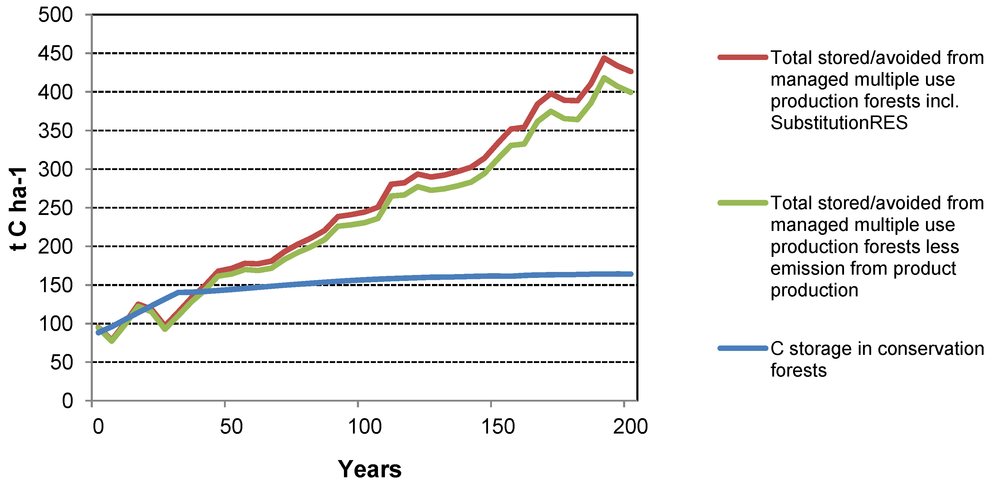
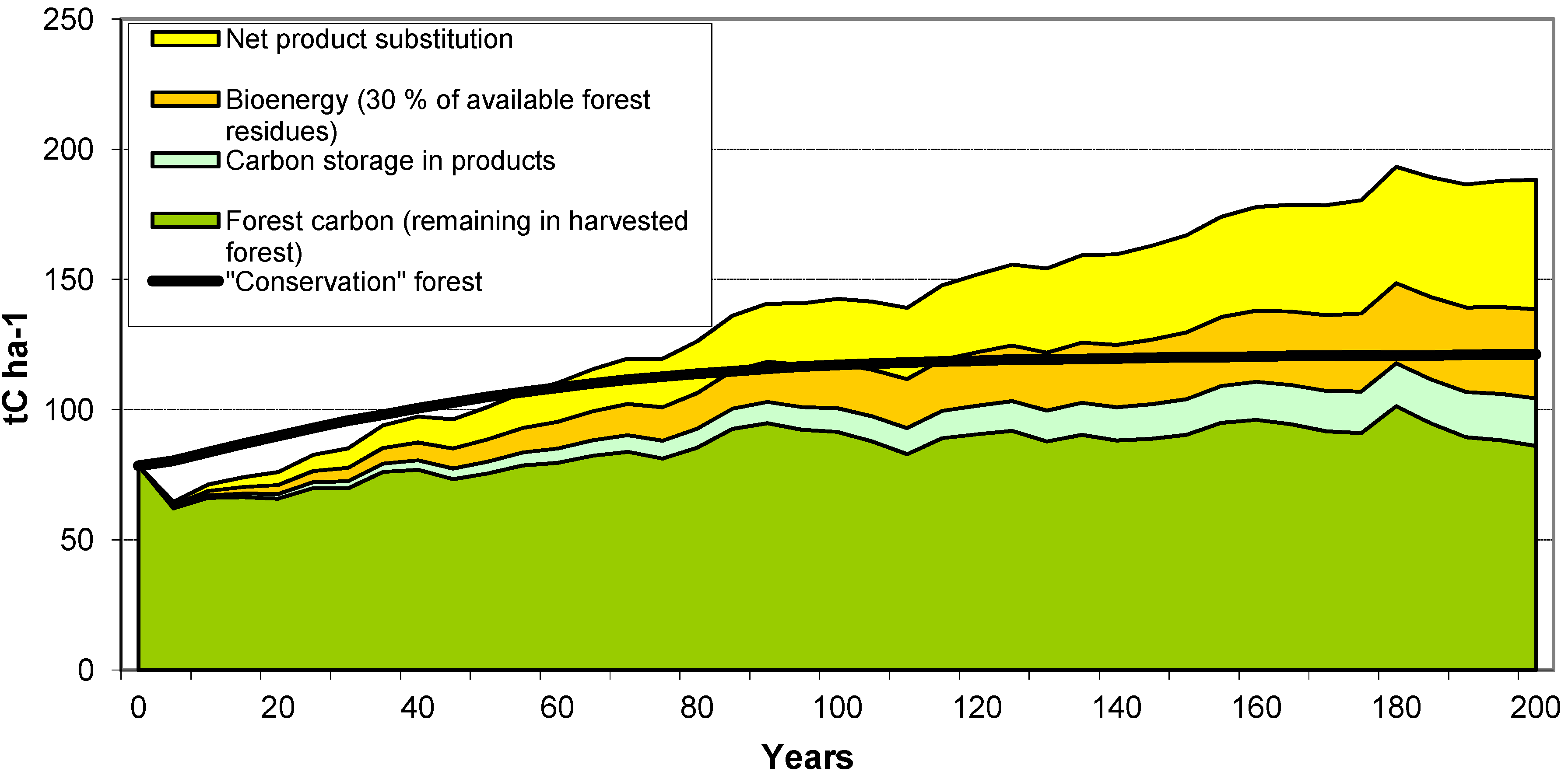
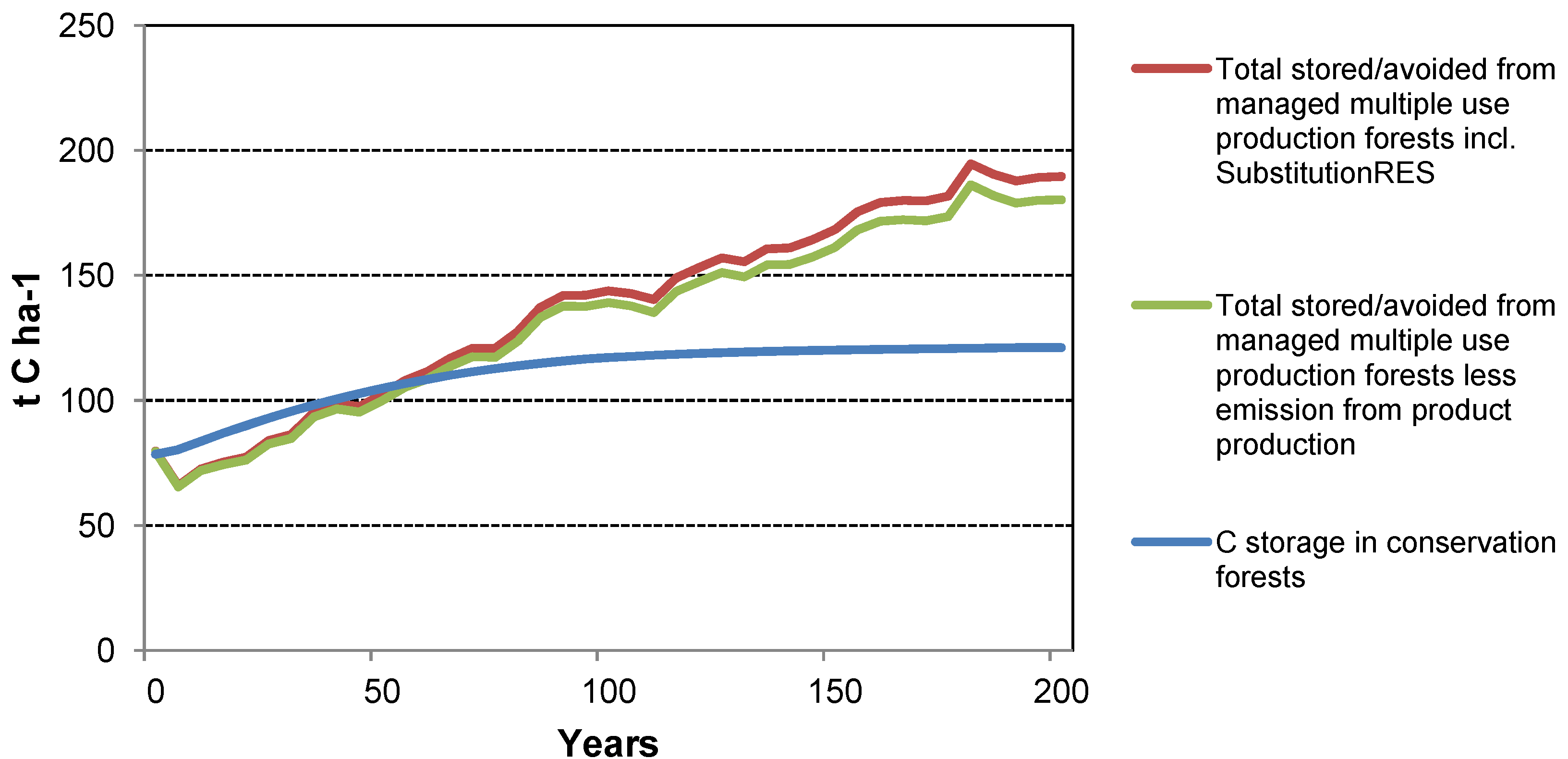
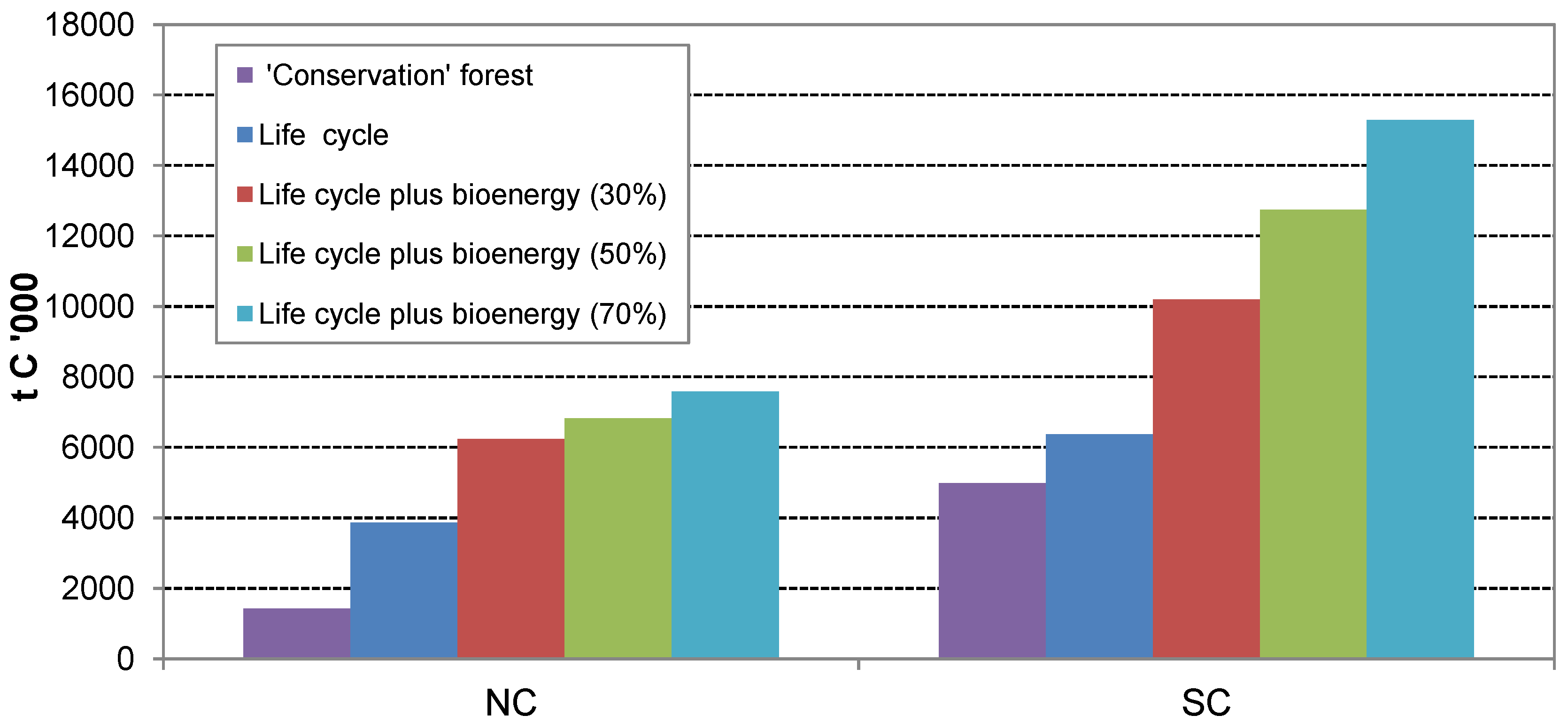
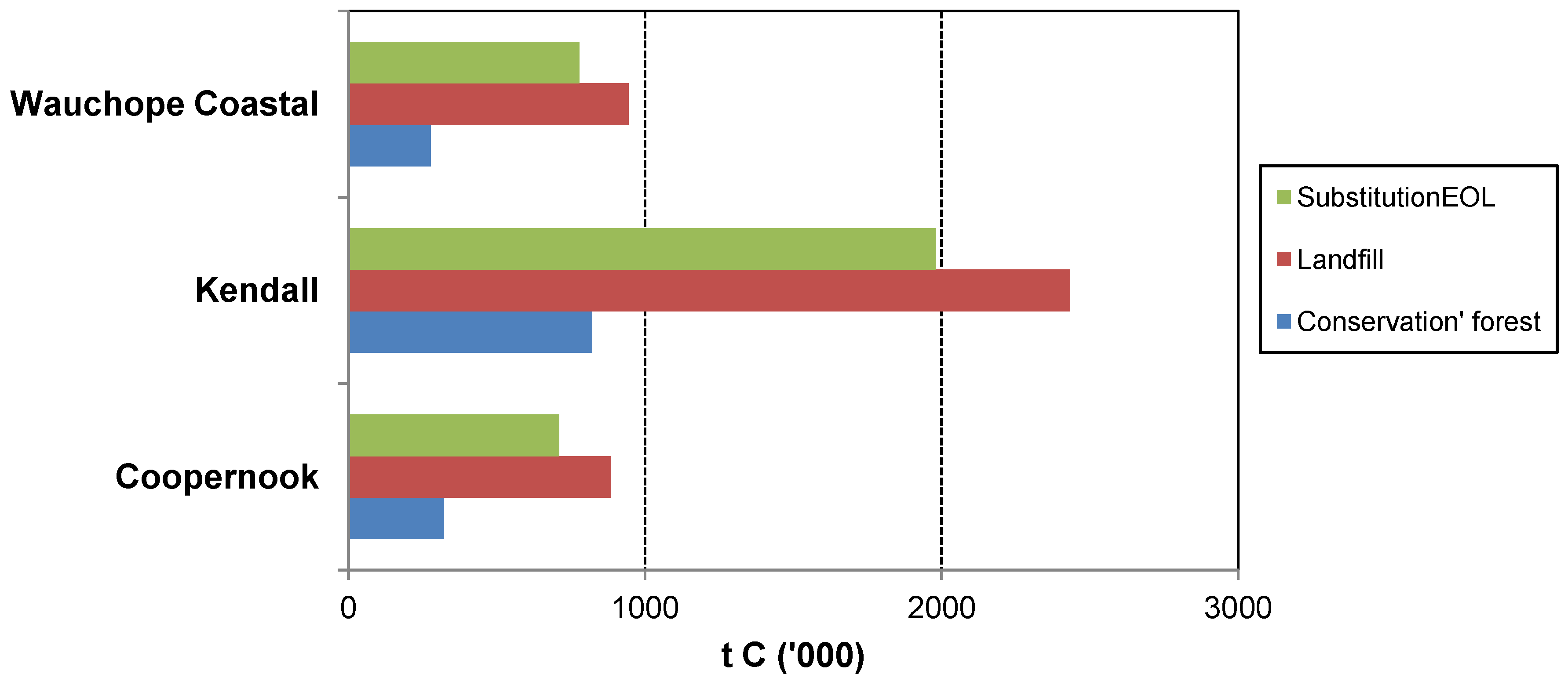
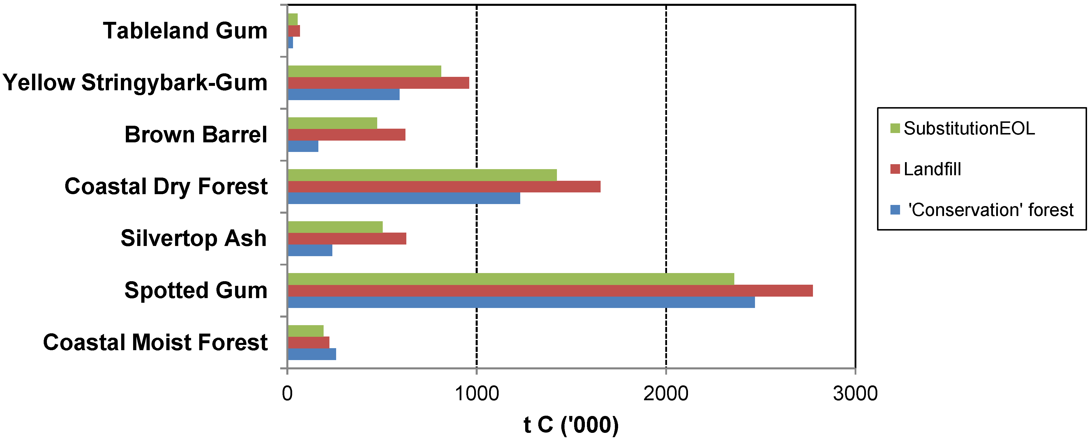
The case studies show that management of forests for wood production has the potential to generate a greater GHG mitigation benefit than managing for conservation alone. Similar conclusions have been drawn by others (e.g., [17,50,51]). Similar to a conservation forest, a multiple-use production forest takes CO₂ from the atmosphere and fixes the C within the tree biomass. However, when biomass is removed at harvest, the C is stored in HWPs while the forest grows more biomass, allowing removal of more biomass in more HWPs in future harvests. After several harvest cycles, more C is stored in the forest plus through the use of HWPs than if the forest had not been harvested. These benefits are realized regardless of the waste management strategy assumed for the case studies (i.e., whether HWPs are disposed off in landfills or incinerated with energy recovery). Although the most recent research in the area of decomposition of HWPs in landfills strongly suggests that solid HWPs and products such as particleboard and MDF (medium-density fiberboard) do not decay to any significant extent [8], in this paper it was conservatively assumed that some decomposition has occurred [6]. In addition, it is assumed that none of the methane generated is either flared or captured to generate electricity-despite the fact that most of the waste produced in Australia is deposited in modern landfills, which typically capture 50%–75% of methane generated to produce electricity [38]. The assumptions for Substitution_EOL adopted here were based on international industry-average incinerator technology producing electricity alone [46] as no waste-to-energy plants are currently operating in Australia. Modern plants using gasification, or combined heat and power, could have an even greater efficiency and therefore an increased net GHG mitigation benefit.

Furthermore, the case studies show that Substitution_HWP provides greater GHG mitigation benefit than the value of C storage in products, as also reported by other researchers (e.g., [17,52,53]). Care should be exercised though when calculating Substitution_HWP to ensure that the increased use of wood will not result in a net loss of forest area due to unsustainable levels of harvest; and that realistic substitution scenarios are used [54]. It is possible that in some instances the use of HWPs will displace the use of less GHG-intensive materials. In this paper the GHG impacts of reduced availability of wood products are demonstrated—not the GHG implications of increased use of wood products. Thus, the risk of a decrease in harvest or wood production elsewhere is not relevant for this discussion. The role of green building schemes in achieving real product substitution would be especially important in the scenario where an increased production of HWPs is assessed.

The GHG implications of not producing paper products from the “production” forests were not taken into account. It is possible that a proportion of the displaced paper products, that would need to be sourced elsewhere if harvest of native forests decreased significantly, would be sourced from areas where unsustainable forestry practices are adopted. This would lead to increased GHG emissions associated with the “conservation” scenario.

The case studies illustrate that the abatement benefit would be enhanced by using a portion of the harvest residues for energy (Substitution_RES), as previously demonstrated in other studies [17,50]. The estimates of emissions offset due to displacement of fossil energy emissions are made for a case where policies or programs result in full displacement of fossil energy (rather than just increasing the total primary energy use). In this context, policies that support increased use of renewable energy (e.g., [19]) are essential to achieve real fossil fuel displacement. If a proportion of harvest residues are used for bioenergy generation to replace fossil fuels, Substitution_RES needs to take into account associated GHG emissions due to fuel usage in the extraction and transport of biomass. These same residues if left in the forest result in gradual emissions of biogenic C over time, and a “lost opportunity” of fossil fuel displacement. Sathre and Gustavsson [55] examined the radiative forcing impact in their analysis of the climate impacts of using forest biomass as biofuel, in order to account for this temporal pattern of C emissions and uptakes. Using this approach, they demonstrated that use of residues as biofuel results in a significant GHG mitigation benefit when compared to natural decay in the forest. Of all the factors impacting on the climate benefits of using harvest residues for bioenergy, the quantity of biomass produced and recovered and the type of fossil fuel replaced, are the most important. In Australia, where currently a large volume of harvest residue is underutilized and where coal is the main source of energy, the GHG mitigation benefit of utilizing harvest residues for bioenergy generation is especially significant.

The C stocks for the NC and SC “conservation” forests were considerably lower than the mean value predicted by Mackey et al. [56] for SE Australian forests undisturbed by harvesting, but within the typical range of values reported for mature native forests in Australia [35,57,58,59,60,61,62]. The estimated C stocks for mature native forests will likely have little impact on the relative difference between the “conservation” and “production” options. A higher C stock in the “conservation” forest at year 200 implies greater forest productivity than that of the forests used for the case studies—this would in most cases also apply to the harvested forest scenario. As a result, both the forest C stocks and off-site GHG mitigation benefits, such as HWPs, would also increase.

Inclusion of C in coarse woody debris (CWD), dead standing wood and fine litter would increase the C stocks for the “conservation” forest scenario by approximately 25 t C ha⁻¹, assuming that published figures for forest types similar to those included the SC study areas [60] can be applied here (similar published data was not found for forests comparable to those included in the NC case study area). Although this would reduce the combined forest and offset C GHG balance for the SC forests by approximately 25% (Table 8), the overall GHG outcome of the SC “production” forest is still significantly better (75 t C ha⁻¹) than that of the SC “conservation” forests. The magnitude of the difference in the GHG balance between NC “production” and “conservation” forests was such (249.5 t C ha⁻¹) that inclusion of C in CWD would result in, proportionally, even less significant changes to the overall GHG outcome.

Although the GHG impact of fires is large over time (even discounting biogenic CO₂ emissions), their effect is more pronounced for “conservation” forests, as the proportion of fire events represented by wildfires was greater for those forests. This resulted in higher estimates of GHG emissions. The impact of including non-CO₂ GHG emissions is significant—the net GHG outcome for NC “conservation” forests at year 200 is nullified, and it becomes negative for SC “conservation” forests. A more accurate calculation of the impact of fire on carbon balance requires better field data as well as modeling—using average fuel consumption rates will reduce the reliability of estimates of GHG emissions from fire [23].

Internationally the focus of Reducing Emissions from Deforestation and Forest Degradation (REDD) projects is justifiably on achieving emission reductions through avoided deforestation and increased forest protection. However, this focus is not applicable in countries where sustainable forest management is adopted, such as Australia. The perception that cessation of harvest in native forests in Australia will provide substantial GHG abatement has led to pressure to convert production forests to conservation forests. Policy being enacted through the Australian Federal Parliament, that potentially will provide credit for cessation of harvest [63] and does not recognise native forest biomass as eligible to earn renewable energy credits [64], does not adequately recognise the nature of C flows in managed forests and hence undervalues their role in GHG mitigation. These policies fail to recognise the potential mitigation benefit of forests harvested for timber and biomass for energy. Lack of recognition of the GHG mitigation benefit of sustainable forest management will limit the potential mitigation that could be achieved by policies that acknowledge and support production of HWPs and use of forest biomass for renewable energy (ideally through mechanisms such as green building certification programs and renewable energy standards). Abatement provided by forest sequestration, HWPs and bioenergy has low cost compared with the cost of abatement through many other measures [65]. Cessation of harvest in some native forests will give no additional mitigation benefits over business as usual (BAU), and will represent a missed opportunity to maintain and potentially enhance forests positive mitigation role and also to support socio-economic development in regional Australia. The findings of the case studies will apply equally to plantations: management of plantations for production of HWPs and bioenergy will deliver a greater GHG mitigation benefit than unharvested plantings.

It has been suggested [66] that HWPs from native forests in Australia could be replaced with products from the existing plantation estate, which would avoid the use of GHG-intensive non-wood products. However, the existing NSW plantation estate has not expanded at the anticipated rate, and the species grown are not suitable for replacing the products such as flooring and external decking, for which native forest timbers are used. Therefore, if other HWPs are to replace native forest timbers these are likely to be imported, with a significant risk of “leakage” through increased emissions from forests harvested (often unsustainably) outside Australia. Much of Australia’s hardwood imports are derived from south-east Asia, predominantly Indonesia [67], where the rate of deforestation (primarily due to logging) is about 1.1 M ha per year, and this is anticipated to increase [67]. Indonesia’s emissions due to deforestation, excluding emissions from peatland fire and oxidation, averaged about 850 Mt per year in the period 2000–2004 [68]. While the Indonesian Government is taking action to promote sustainable forest management [68] increased imports of tropical hardwood timber by Australia are likely to be supplied at least partially from deforestation. Thus, the current GHG policy direction in Australia in relation to forests has the potential to result in increased net global emissions, due to the need for GHG-intensive alternative products and/or the import of HWPs from unsustainably managed forests. This risk is clearly identified by Kastner et al. [69], who state that “policies aiming at increasing national forest stocks, should include careful assessments if and to what extent this forest return will be facilitated by increasing risks and vulnerabilities in distant places”.

The case study findings demonstrate the importance of considering the entire forestry system, from a life cycle perspective. Upstream, downstream and indirect effects need to be accounted for when assessing the GHG impacts of forest management decisions. While it may be efficient to address environmental objectives such as water management, biodiversity conservation and GHG management simultaneously, striving for synergistic outcomes, there are inevitably tradeoffs [70]. These should be made transparent and explicit. In devising policy measures to meet environmental and production objectives, governments should be mindful of the need to provide clear and consistent policy, to encourage industry to develop low GHG products and energy systems including bioenergy [71].

5. Conclusions

When quantifying the climate change impacts of alternative forest management options it is critical to consider the whole forest system, including indirect impacts of management decisions in order to reduce the risk of perverse environmental outcomes. Multiple-use native forests could play a significant role in climate change mitigation when managed for production of wood and non-wood products including biomass for bioenergy.

The following key conclusions are drawn from the case studies:

• (1) Whilst for a specific site and point in time, the C stored in a forest reserved for conservation may be greater than in a harvested forest, in the long term, when the full GHG balance is considered, multiple-use production forests have significantly larger GHG abatement potential than conservation forests. Proper consideration of substitution benefits and leakage potential is critical in this assessment.
• (2) There is a need to explore opportunities associated with limited extraction of harvest slash (residues) for bioenergy (taking into account biodiversity and forest nutrition needs). This limited extraction has potentially large GHG mitigation benefits associated with replacing coal-based emissions from electricity generation.
• (3) Irrespective of the end of life path for HWPs (e.g., recycling, landfill or energy recovery systems) the GHG outcome from harvested forests will be positive compared with conservation forests.
• (4) Managing the forests so they grow productively is important for sustained mitigation benefit, as is ensuring timber is processed to long-life products and can be utilised to offset fossil-fuel emissions at the end of their lifespan.
• (5) A key finding of this study is that current policy directions in Australia towards returning more of the “production” forest estate into “conservation” areas on the basis of perceived GHG benefits will have perverse outcomes in the long-term, resulting in increased GHG emissions.

The case studies highlighted key gaps or limitations in current data, such as the impact of wildfires and prescribed burning on long-term GHG emissions; implications of extraction of residues on below ground C dynamics; the role of CWD and the need for regionalised scenarios for Substitution_HWP and for potential leakage impacts, as the substitution scenarios may change significantly from region to region depending on market conditions. Although the nature of the overall impact of including the effect of regular fire events and management of residues on C stocks in the case studies outlined here is clear (i.e., they will favour the “production” scenario), insufficient data are currently available to underpin more refined assessments. These limitations should be addressed in future research.

References

1. ABARES (Australian Bureau of Agricultural and Resources Economics and Sciences). Australia’s Forests at a Glance 2011—With Data to 2009-2010; Commonwealth of Australia: Canberra, Australia, 2011. Available online: http://adl.brs.gov.au/data/warehouse/pe_abares99001800/Forests_at_a_glance_2011.pdf (accessed on 23 March 2012).
2. Commonwealth of Australia. National Forest Policy Statement: A New Focus for Australia’s Forests. 1992. Available online: http://www.daff.gov.au/__data/assets/pdf_file/0019/37612/nat_nfps.pdf (accessed on 23 March 2012).
3. Resource Assessment Commission (RAC), A Survey of Australia’s Forest Resource; Australian Government Public Service: Canberra, Australia, 1992.
4. Forests NSW. Forests New South Wales Annual Report 2009–2010—Social, Environmental and Economic Performance; New South Wales Government: New South Wales, Australia, 2010. Available online: http://www.dpi.nsw.gov.au/__data/assets/pdf_file/0009/366750/forests-nsw-annual-report-200910-complete.pdf (accessed on 23 March 2012).
5. Ximenes, F.; Gardner, W.D.; Kathuria, A. Proportion of above-ground biomass in commercial logs and residues following the harvest of five commercial forest species in Australia. For. Ecol. Manag. 2008, 256, 335–346. [Google Scholar] [CrossRef]
6. Ximenes, F.A.; Gardner, W.D.; Cowie, A. The decomposition of wood products in landfills in Sydney, Australia. Waste Manag. 2008, 28, 2344–2354. [Google Scholar] [CrossRef]
7. Eggleston, S.; Buendia, L.; Miwa, K.; Ngara, T.; Tanabe, K. (Eds.) Intergovernmental Panel on Climate Change (IPCC). Waste. Guidelines for National Greenhouse Gas Inventories; Institute for Global Environmental Strategies: Hayama, Japan, 2006; 5, pp. 3.13–3.15. Available online: http://www.ipcc-nggip.iges.or.jp/public/2006gl/vol5.html (accessed on 23 March 2012).
8. Wang, X.; Padgett, J.M.; De la Cruz, F.B.; Barlaz, M.A. Wood biodegradation in laboratory scale landfills. Environ. Sci. Technol. 2011, 45, 6864–6871. [Google Scholar]
9. Ximenes, F.A. Carbon Storage in Wood Products in Australia: A Review of the Current State of Knowledge; Project No. PR06.5044; Report prepared for the Forest and Wood Products Research and DevelopmentCorporation: Melbourne, Australia, 2006. [Google Scholar]
10. Mclennan Magasanik Associates, Energy Usage in Timber Framing; Report to the National Association of Forest Industries: Albert Park, Australia, 1991.
11. Buchanan, A.H.; Levine, S.B. Wood-based building materials and atmospheric carbon emissions. Environ. Sci. Pol. 1999, 2, 427–437. [Google Scholar] [CrossRef]
12. Ximenes, F.; Grant, T. Quantifying the Carbon Benefits of Use of Wood Products in Home Construction Using a Life Cycle Assessment Approach; Report to the NSW Department of Environment and Climate Change: Sydney, Australia, 2009.
13. May, A.; England, J.R.; Raison, J.R.; Paul, K.I. Cradle-to-gate inventory of wood production from Australian softwood plantations and native hardwood forests: Embodied energy, water use and other inputs. For. Ecol. Manag. 2011, 264, 37–50. [Google Scholar]
14. Sathre, R.J.; O’Connor, J. Meta-analysis of greenhouse gas displacement factors of wood product substitution. Environ. Sci. Pol. 2010, 13, 104–114. [Google Scholar] [CrossRef]
15. Gustavsson, L.; Pingoud, K.; Sathre, R. Carbon dioxide balance of wood substitution: Comparing concrete and wood-framed buildings. Mitig. Adapt. Strateg. Glob. Change 2006, 11, 667–691. [Google Scholar] [CrossRef]
16. Perez-Garcia, J.; Lippke, B.; Comnick, J.; Manriquez, C. An assessment of carbon pools, storage, and wood products market substitution using life-cycle analysis results. Wood Fib. Sci. 2005, 37, 140–148. [Google Scholar]
17. Lippke, B.; Oneil, E.; Harrison, R.; Skog, K.; Gustavsson, L.; Sathre, R. Life cycle impacts of forest management and wood utilisation on carbon mitigation: knowns and unknowns. Carbon Manag. 2011, 2, 303–333. [Google Scholar] [CrossRef]
18. Nabuurs, G.; Ravindranath, N.H.; Paustian, K.; Freibauer, A.; Hohenstein, W.; Makundi, W. (Eds.) Intergovernmental Panel on Climate Change (IPCC). Chapter 3, Section3.2 Forest Land. Good Practice Guidance for LULUCF; IPCC National Greenhouse Gas Inventories Programme: Hayama, Japan, 2003. Available online: http://www.ipcc-nggip.iges.or.jp/public/gpglulucf/gpglulucf_files/Chp3/Chp3_2_Forest_Land.pdf (accessed on 23 March 2012).
19. Commonwealth of Australia. Renewable Energy Amendment Act 2009; Australian Government Amendment Act 2009 No. 78: Canberra, Australia, 2009. Available online: http://www.comlaw.gov.au/Details/C2009A00078. (accessed on 23 March 2012).
20. Australian Bureau of Agricultural and Resources Economics and Sciences (ABARES). Australian Energy National and State Projections to 2029–2030; ABARE Research Report 06.26; Commonwealth of Australia: Canberra, Australia, 2007. Available online: http://adl.brs.gov.au/data/warehouse/pe_abare99001338/arr06.26_energy_projections.pdf (accessed on 23 March 2012).
21. Bradstock, R.A.; Williams, J.A.; Gill, A.M. Flammable Australia—Ecology and Biodiversity of a Continent, 1st ed; Cambridge University Press: Cambridge, UK, 2002. [Google Scholar]
22. Ellis, S.; Kanowski, P.; Whelan, R. National Inquiry on Bushfire Mitigation and Management; Commonwealth of Australia: Canberra, Australia, 2004. [Google Scholar]
23. Gould, J.; Cheney, P. Fire Management in Australian Forests. In Forest Management in Australia: Implications for Carbon Budgets; NCAS Technical Report No. 32; Raison, R.J., Squire, R.O., Eds.; Australian Greenhouse Office: Canberra, Australia, 2007; Volume 1, pp. 341–388. [Google Scholar]
24. Raison, R.J.; Kirschbaum, M.U.F.; McCormack, R.J.; Attiwill, P.M.; Richardson, A.M.M. Review of the Science Relevant to the Sustainable Use of Forest Harvesting Residues for Energy Production in Tasmania; CSIRO Client Report No. 1122 for Forestry Tasmania; National Power, John Holland Development and Investments: Canberra, Australia, 2002. [Google Scholar]
25. Florence, R.G. Ecology and Silviculture of Eucalypt Forests; CSIRO: Collingwood, Australia, 1996. [Google Scholar]
26. Florence, R. New South Wales. In Forest Management in Australia: Implications for Carbon Budgets; NCAS Technical Report No. 32; Raison, R.J., Squire, R.O., Eds.; Australian Greenhouse Office: Canberra, Australia, 2007; Volume 1, pp. 49–102. [Google Scholar]
27. State Forests of NSW, Biometric Models: Upper North East and Lower North East CRA Regions; Project number: NA13/FRA; A project undertaken for the Joint Commonwealth NSW Regional Forest Agreement Steering Committee: New South Wales, Australia, 2000.
28. Vanclay, J. Review of Projected Timber Yields for the NSW North Coast, Southern Cross University: Lismore, Australia, 2002; Unpublished work.
29. Audit Office of New South Wales (NSW). Sustaining Native Forest Operations. Forests NSW: Sydney, Australia, 2009. Available online: http://auditofficestaging.elcom.com.au/ArticleDocuments/141/185_Sustaining_Native_Forest.pdf.aspx?Embed=Y (accessed on 23 March 2012).
30. Ximenes, F.; Gardner, W.D.; Marchant, J.F. Carbon Flow Following the Harvest of Blackbutt Trees and Their Conversion into Sawn Products; Research Paper No. 41; NSW Department of Primary Industries: Sydney, Australia, 2005. [Google Scholar]
31. Scherl, T. At the Crossroads: A Comparison of Social, Scientific and Political Influences on Fire Management in the US and in Australia; Report for the World Forest Institute: Portland, OR, USA, 2005. Available online: Available online: http://wfi.worldforestry.org/media/publications/specialreports/Fire_Mngt_Scherl.pdf. (accessed on 23 March 2012).
32. Department of Climate Change and Energy Efficiency (DCCEE). Australian National Greenhouse Accounts National Inventory Report 2009; The Australian Government Submission to the UN Framework Convention on Climate Change, Commonwealth of Australia: Canberra, Australia, 2011. Available online: http://www.climatechange.gov.au/publications/greenhouse-acctg/~/media/publications/greenhouse-acctg/national-inventory-report-2009-vol2.pdf (accessed on 23 March 2012).
33. Price, O.F.; Bradstock, R.A. Quantifying the influence of fuel age and weather on the annual extent of unplanned fires in the Sydney region of Australia. Int. J. Wildland Fire 2011, 20, 142–151. [Google Scholar]
34. Ximenes, F.A.; Gardner, W.D.; Marchant, J.F. Total Biomass Measurement and Recovery of Biomass in Log Products in Spotted Gum (Corymbia maculata) Forests of SE NSW; National Carbon Accounting System Technical Report No. 47; Australian Greenhouse Office: Canberra, Australia, 2005. Available online: http://pandora.nla.gov.au/pan/23322/20080818-0001/www.climatechange.gov.au/ncas/reports/tr47final.html (accessed on 23 March 2012).
35. Ximenes, F.A.; Davies, I. TimberCAM—A Carbon Accounting Model for Wood and Wood Products; User’s Guide; Cooperative Research Centre for Greenhouse Accounting: Canberra, Australia, 2004. Available online: http://www.dpi.nsw.gov.au/forests/info/timbercam (accessed on 23 March 2012).
36. Tucker, S.; Tharumarajah, A.; May, B.; England, J.; Paul, K.; Hall, M.; Mitchell, P.; Rouwette, R.; Seo, S.; Syme, M. Life Cycle Inventory of Australian Forests and Wood Products; Project No. PNA008-0708; Report for Forests and Wood Products Australia: Melbourne, Australia, 2009. [Google Scholar]
37. Ximenes, F.; Brooks, P. The Greenhouse Footprint of Wood Products in NSW; Final Report for the New South Wales Government Climate Action Grant Project “T06/CAG/028”: Sydney, Australia, 2010. [Google Scholar]
38. Hyder Consulting, Comparative Greenhouse Gas Life Cycle Assessment of Wollert Landfill, Report prepared for Hanson Landfill Services and the City of Whittlesea: Melbourne, Australia, 2010.
39. Johnson, D.W.; Curtis, P.S. Effects of forest management on soil C and N storage: Meta analysis. For. Ecol. Manag. 2001, 140, 227–238. [Google Scholar] [CrossRef]
40. Rodriguez, L.C.; May, B.; Herr, A.; O’Connell, D. Biomass assessment and small scale biomass fired electricity generation in the Green Triangle, Australia. Biomass Bioenerg. 2011, 35, 2589–2599. [Google Scholar] [CrossRef]
41. Hansson, J.; Berndes, G.; Johnsson, F.; Kjärstad, J. Co-firing biomass with coal for electricity generation—An assessment of the potential in EU27. Energy Policy 2009, 37, 1444–1455. [Google Scholar]
42. Department of Climate Change and Energy Efficiency (DCCEE), National Greenhouse Factors; Commonwealth of Australia: Canberra, Australia, 2010.
43. ECN-Biomass. Energy Research Centre of the Netherlands. Available online: http://www.ecn.nl/phyllis/ (accessed on 23 March 2012).
44. Peck, A.; Sudmeyer, R.; Huxtable, D.; Bartle, J.R.; Mendham, D.S. Productivity of Mallee Agroforestry Systems under Various Harvest and Competition Management Regimes; Reportprepared for the Rural Industries Research and Development Corporation (RIRDC): Canberra, Australia, 2012; in print. [Google Scholar]
45. Lenzen, M. Life cycle energy and greenhouse gas emissions of nuclear energy: A review. Energy Convers. Manag. 2008, 49, 2178–2199. [Google Scholar] [CrossRef]
46. Denison, R.A. Environmental life-cycle comparisons of recycling, landfilling and incineration: A review of recent studies. Annu. Rev. Energy Environ. 1996, 21, 191–237. [Google Scholar] [CrossRef]
47. Stupak, I.; Lattimore, B.; Titus, B.D.; Tattersall Smith, C. Criteria and indicators for sustainable forest fuel production and harvesting: A review of current standards for sustainable forest management. Biomass Bioenerg. 2011, 35, 3287–3308. [Google Scholar] [CrossRef]
48. Lattimore, B.; Smith, C.T.; Titus, B.D.; Stupak, I.; Egnell, G. Environmental factors in woodfuel production: Opportunities, risks, and criteria and indicators for sustainable practices. Biomass Bioenerg. 2009, 33, 1321–1342. [Google Scholar]
49. Farine, D.R.; O’Connell, D.A.; Raison, J.; May, B.; O’Connor, M.H.; Crawford, D.F.; Herr, A.; Taylor, J.A.; Jovanovic, T.; Campbell, P.K.; et al. An assessment of biomass for bioelectricity and biofuel, and for greenhouse gas emission reduction in Australia. Glob. Change Biol. Bioenergy 2012, 4, 148–175. [Google Scholar] [CrossRef]
50. Schlamadinger, B.; Canella, L.; Marland, G.; Spitzer, J. Bioenergy strategies and the global carbon cycle. Sci. Geol. Bull. 1997, 50, 157–182. [Google Scholar]
51. Eriksson, E.; Gillespie, A.R.; Gustavsson, L.; Langvall, O.; Olsson, M.; Sathre, R. Integrated carbon analysis of forest management practices and wood substitution. Can. J. For. Res. 2007, 37, 671–681. [Google Scholar] [CrossRef]
52. Kauppi, P.; Sedjo, R. Technological and Economic Potential of Options to Enhance, Maintain, and Manage Biological Carbon Reservoirs and Geo-engineering. Climate Change 2001: Mitigation, IPCC Third Assessment Report Vol.3; Metz, B., Davidson, O., Swart, R., Pan, J.H., Eds.; Academic Press: New York, NY, USA, 2001. Available online: http://www.grida.no/climate/ipcc_tar/wg3/index.html (accessed on 23 March 2012).
53. Perez-Garcia, J.; Lippke, B.; Briggs, D.; Wilson, J.B.; Boyer, J.; Meil, J. The environmental performance of renewable building materials in the context of residential construction. Wood Fib. Sci. 2005, 37, 3–17. [Google Scholar]
54. Law, B.E.; Harmon, M.E. Forest sector carbon management, measurement and verification, and discussion of policy related to climate change. Carbon Manag. 2011, 2, 73–84. [Google Scholar] [CrossRef]
55. Sathre, R.J.; Gustavsson, L. Time-dependent climate benefits of using forest residues to substitute fossil fuels. Biomass Bioenerg. 2011, 35, 2506–2516. [Google Scholar] [CrossRef]
56. Mackey, B.G.; Keith, H.; Berry, S.L.; Lindenmayer, D.B. Green Carbon: The Role of Natural Forests in Carbon Storage, Part 1. A Green Carbon Account of Australia’s Southeastern Eucalypt Forests, and Policy Implication; Australian National University: Canberra, Australia, 2008. Available online: http://epress.anu.edu.au/titles/green-carbon/pdf-download (accessed on 23 March 2012).
57. Turner, J.; Lambert, M.J. Effects of forest harvesting nutrient removals on soil nutrient reserves. Oecologia 1986, 70, 140–148. [Google Scholar] [CrossRef]
58. Grierson, P.; Adams, M.A.; Attiwill, P. Estimates of carbon storage in the above-ground biomass of Victoria’s forests. Aust. J. Bot. 1993, 40, 631–640. [Google Scholar]
59. Raison, J.; Keith, H.; Barrett, D.; Burrows, B.; Grierson, P. Spatial Estimates of Biomass in “Mature” Native Vegetation; National Carbon Accounting System Technical Report No. 44; Australian Government, Australian Greenhouse Office: Canberra, Australia, 2003. Available online: http://pandora.nla.gov.au/pan/23322/200502180000/www.greenhouse.gov.au/ncas/reports/tr4final.html (accessed on 23 March 2012).
60. Roxburgh, S.H.; Wood, S.W.; Mackey, B.G.; Woldendorp, G.; Gibbons, P. Assessing the carbon sequestration potential of managed forests: A case study from temperate Australia. J. Appl. Ecol. 2006, 43, 1149–1159. [Google Scholar] [CrossRef]
61. Moroni, M.T.; Kelley, T.H.; McLarin, M.L. Carbon in trees in Tasmanian State forest. Int. J. For. Res. 2010, 2010. [Google Scholar]
62. Norris, J.; Arnold, S.; Sairman, T. An indicative estimate of carbon stocks on Victoria’s publicly managed land using the FullCAM carbon accounting model. Aust. For. 2010, 73, 209–219. [Google Scholar]
63. Commonwealth of Australia. Carbon Credits (Carbon Farming Initiative) Act 2011; Commonwealth Government Document; Canberra, Australia, 2011. Available online: http://www.comlaw.gov.au/Details/C2011A00101 (accessed on 23 March 2012).
64. Commonwealth of Australia. Renewable Energy (Electricity) Regulations 2001; Australian Parliament: Canberra, ACT, Australia, 2011. Available online: http://www.comlaw.gov.au/Series/F2001B00053 (accessed on 23 March 2012).
65. McKinsey & Company. An Australian Cost Curve for Greenhouse Gas Reduction; McKinsey & Company: Sydney, Australia, 2008. Available online: http://www.gbca.org.au/docs/McKinseyAustralian_Cost_Curve_for_GHG_Reduction[1].pdf (accessed on 23 March 2012).
66. Ajani, J. Australia’s transition from native forests to plantations: the implications for woodchips, pulpmills, tax breaks and climate change agenda. J. Policy Anal. Reform. 2008, 15. Available online: http://epress.anu.edu.au/agenda/015/03/pdf/15-3-AN-2.pdf (accessed on 23 March 2012).
67. Jaakko Poyry Consulting. Overview of Illegal Logging; Report prepared for the Australian Government (51AO5753. 2005): Melbourne, Australia, 2005. Available online: http://www.daff.gov.au/__data/assets/pdf_file/0009/37593/illegal_logging_report_16sept05.pdf (accessed on 23 March 2012).
68. Indonesia Second National Communication under the United Nations Framework Convention on Climate Change; Ministry of Environment, Republic of Indonesia: Jakarta, Indonesia, 2010. Available online: http://unfccc.int/files/national_reports/nonannex_i_natcom/submitted_natcom/application/pdf/indonesia_snc.pdf (accessed on 23 March 2012).
69. Kastner, T.; Erb, K.; Nonhebel, S. International wood trade and forest change: A global analysis. Glob. Environ. Change 2011, 21, 947–956. [Google Scholar] [CrossRef]
70. Cowie, A.L.; Schneider, U.A.; Montanarella, L. Potential synergies between existing multilateral environmental agreements in the implementation of land use, land-use change and forestry activities. Environ. Sci. Pol. 2007, 10, 335–352. [Google Scholar] [CrossRef]
71. George, B.H. Towards 2020: Growing our sustainable future. Biofuels 2012, 3, 115–118. [Google Scholar] [CrossRef]