Effects of Initial Stand Density and Climate on Red Pine Productivity within Huron National Forest, Michigan, USA


Abstract
:1. Introduction
2. Methods
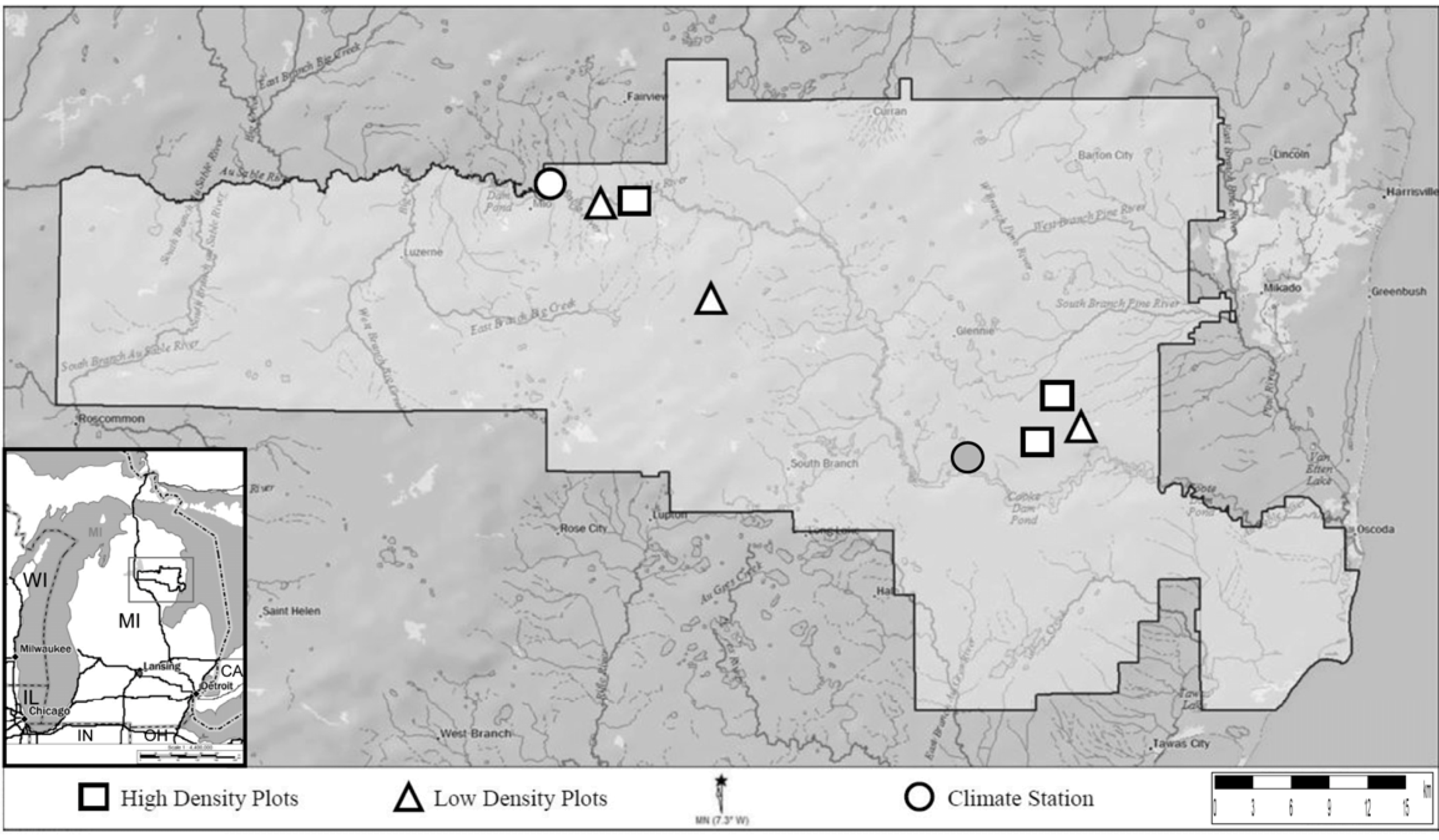
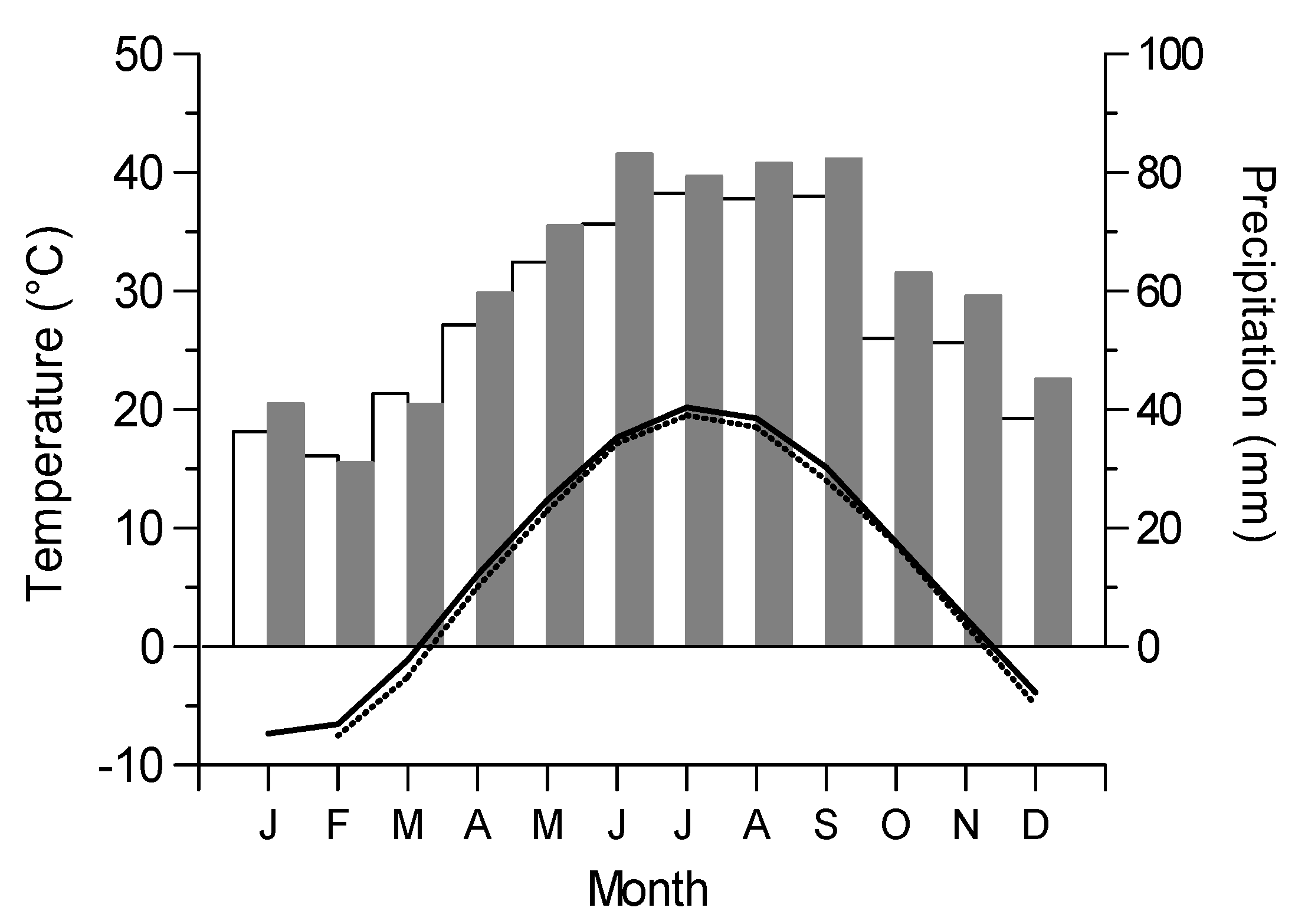
2.1. Study Site


2.2. Field Sampling
2.3. Sample Processing
2.4. Cross-Dating and Treering Measurement
2.5. Data Analysis
2.5.1. Biomass Calculations

- Tbm = total aboveground biomass
- Exp = exponential function
- In = natural log base e (2.718282)
- DBH = diameter at breast height

- Ratio = ratio of stem biomass to total aboveground biomass
- Exp = exponential function
- DBH = diameter at breast height
2.5.2. Red Pine Form and Productivity
2.5.3. Dendrochronological Analysis
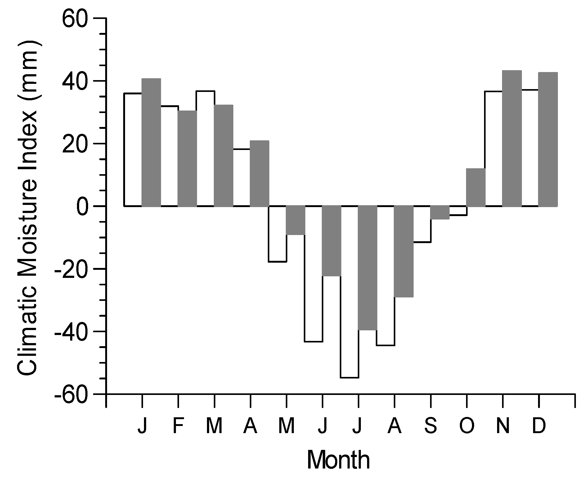
2.5.4. Climate Resilience Index (CRI)

3. Results
3.1. Red Pine Form and Productivity

| Treatment | Age | DBH (cm) | Tree Height (m) | Crown Ratio | Slenderness |
|---|---|---|---|---|---|
| High Density | 57 (10.1) a | 21.6 (3.2) a | 14.12 (0.93) a | 0.350 (0.121) a | 70.5 (11.7) a |
| Low Density | 64 (8.2) a | 28.0 (8.5) a | 17.84 (2.98) a | 0.474 (0.229) a | 68.0 (11.3) a |
| Treatment | Basal Area (m2) | Total Above Ground Biomass (kg) | Total Stem Biomass (kg) |
|---|---|---|---|
| High Density | 0.033 (0.002) a | 127.6 (8.4) a | 80.6 (5.59) a |
| Low Density | 0.057 (0.015) b | 243.5 (81.1) a | 157.0 (53.8) a |
| Treatment | Basal Area (m2/hectare) | Total Above Ground Biomass (Metric Tons/hectare) | Total Stem Biomass (Metric Tons/hectare) |
|---|---|---|---|
| High Density | 44.91 (6.82) a | 183.5 (38.8) a | 116.0 (25.0) a |
| Low Density | 34.48 (6.60) a | 155.6 (20.2) a | 95.0 (17.5) a |

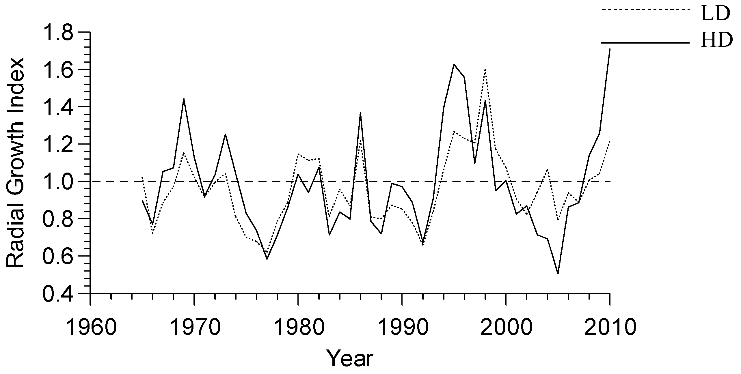
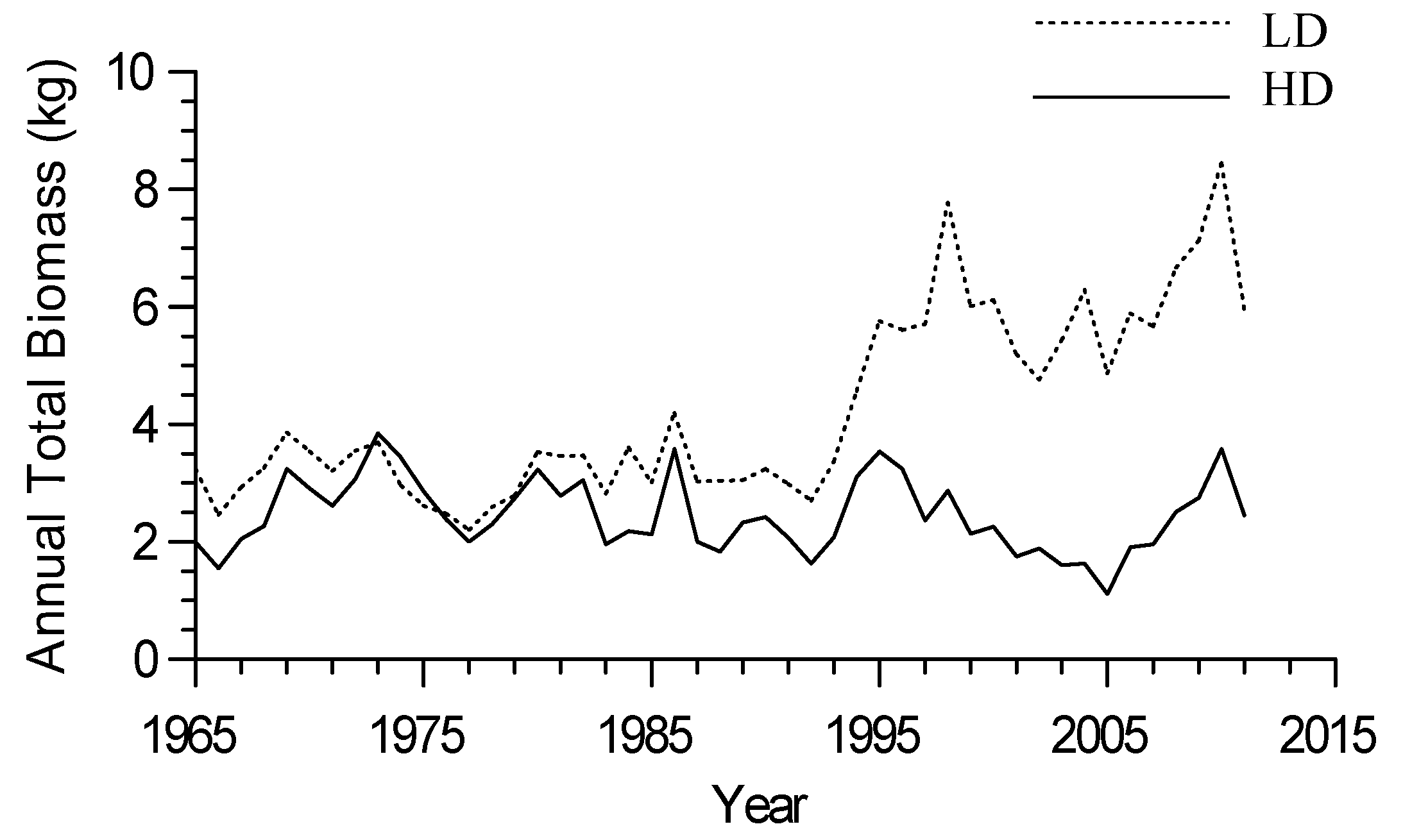
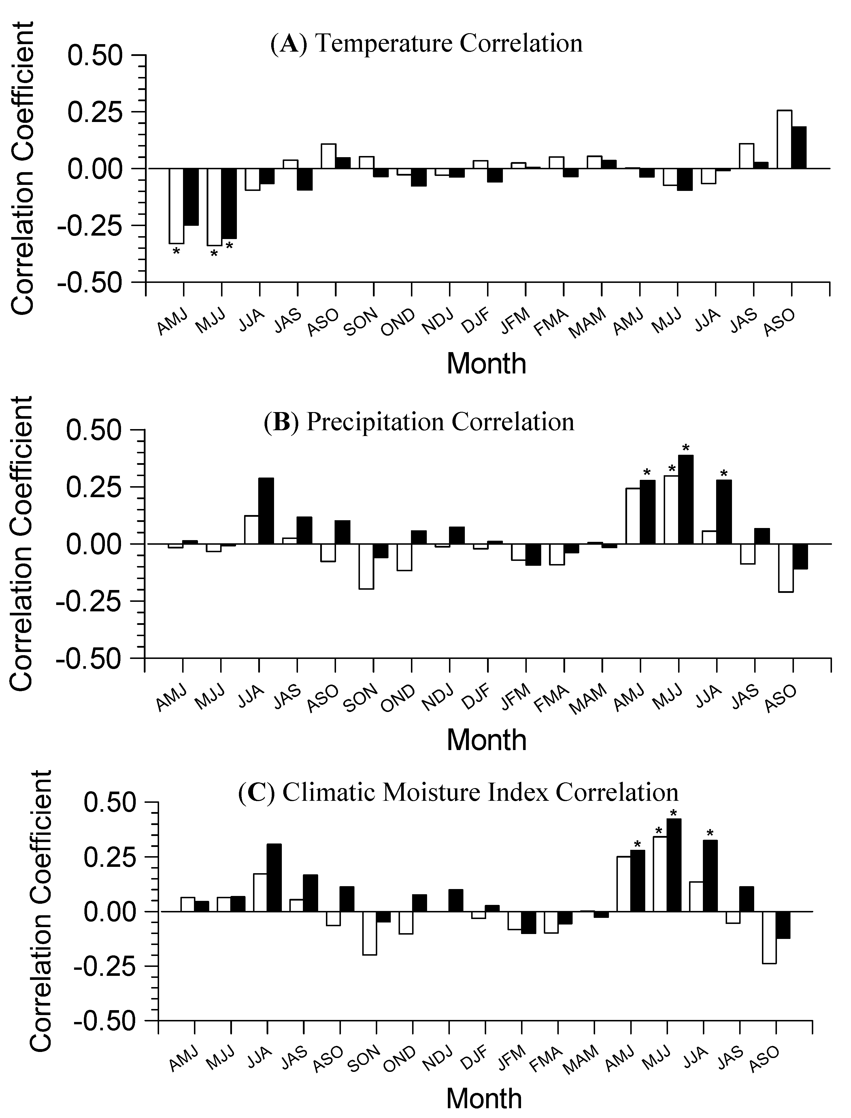
3.2. Growth-Climate Relationships
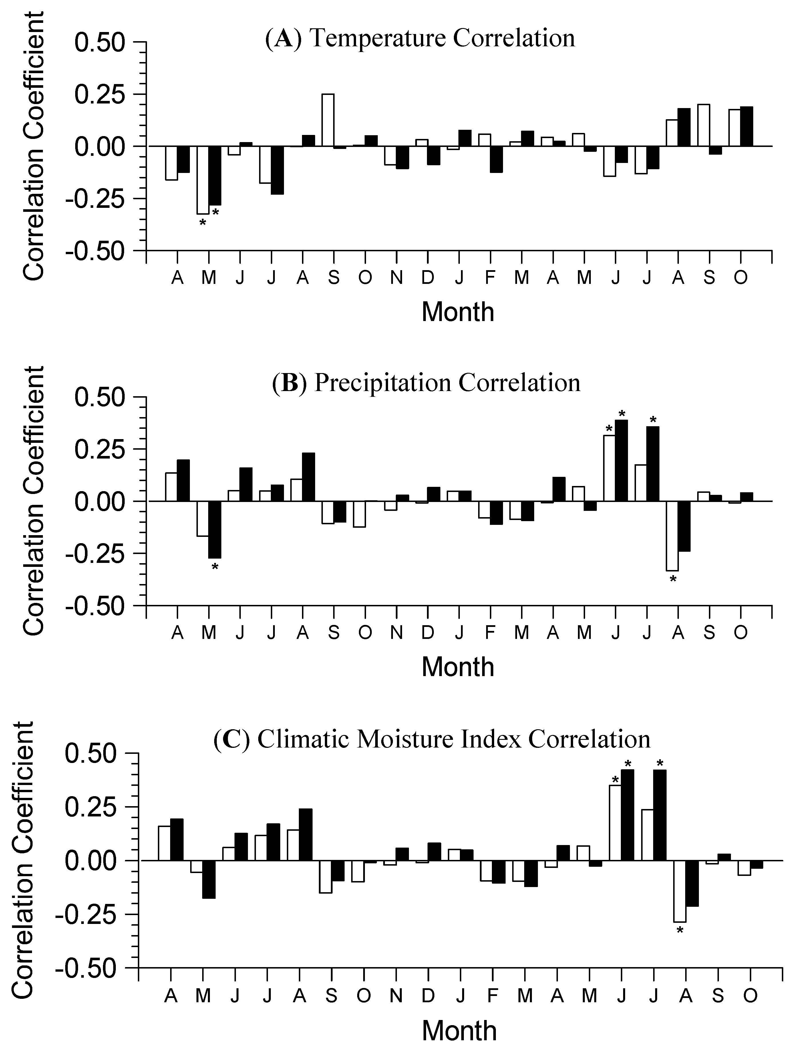

3.3. Climate Resilience Index (CRI)
| Treatment | Stand-Level Productivity (SLP) | Tree-Level Productivity (TLP) | Sensitivity to Monthly Climate (SMC) | Sensitivity to Seasonal Climate (SSC) | Climate Resilience Index (CRI) |
|---|---|---|---|---|---|
| High density | 1.18 | 1.00 | 1.20 | 1.75 | −0.77 |
| Low density | 1.00 | 1.91 | 1.00 | 1.00 | 0.91 |
4. Discussion
4.1. Red Pine Form and Productivity
4.2. Growth-Climate Relationships
4.3. Site Network
4.4. Forest Management and Climatic Resilience
5. Conclusions
Conflict of Interest
Acknowledgements
References
- Chmura, D.J.; Anderson, P.D.; Howe, G.T.; Harrington, C.A.; Halofsky, J.E.; Peterson, D.L.; Shaw, D.C.; St. Claire, J.B. Forest responses to climate change in the northwestern United States: Ecophysiological foundations for adaptive management. For. Ecol. Manag. 2011, 261, 1121–1142. [Google Scholar] [CrossRef]
- Spittlehouse, D.L.; Stewart, R.B. Adaptation to climate change in forest management. BC J. Ecosyst. Manag. 2003, 4, 1–11. [Google Scholar]
- Dombroskie, S.; McKendy, M.; Ruelland, C.; Richards, W.; Bourque, C.P.-A.; Meng, F.-R. Assessing impact of projected future climate on tree species growth and yield: Development of an evaluation strategy. Mitig. Adapt. Strateg. Glob. Chang. 2010, 15, 307–320. [Google Scholar] [CrossRef]
- Gilmore, D.W.; Palik, B.J. A Revised Managers Handbook for Red Pine in North Central Region; USDA Forest Service General Technical Report NC-264; USDA Forest Service: St. Paul, MN, USA, 2005. [Google Scholar]
- Larocque, G.R. Examining different concepts for the development of a distance-dependent competition model for red pine diameter growth using long-term stand data differing in initial stand density. For. Sci. 2002, 48, 24–34. [Google Scholar]
- Penner, M.; Robinson, C.; Burgess, D. Pinus resinosa product potential following initial spacing and subsequent thinning. For. Chron. 2001, 77, 129–139. [Google Scholar]
- Folke, C.; Carpenter, S.; Walker, B.; Scheffer, M.; Elmqvist, T.; Gunderson, L.; Holling, C.S. Regime shifts, resilience, and biodiversity in ecosystem management. Annu. Rev. Ecol. Evol. Syst. 2004, 35, 557–581. [Google Scholar] [CrossRef]
- Millar, C.I.; Stephenson, N.L.; Stephens, S.L. Climate change and forests of the future: Managing in the face of uncertainty. Ecol. Appl. 2007, 17, 2145–2151. [Google Scholar] [CrossRef]
- Chhin, S.; Hogg, E.H.; Lieffers, V.J.; Huang, S. Potential effects of climate change on the growth of lodgepole pine across diameter size classes and ecological regions. For. Ecol. Manag. 2008, 256, 1692–1703. [Google Scholar] [CrossRef]
- Kipfmueller, K.F.; Elliot, G.P.; Larson, E.R.; Salzer, M.W. An assessment of the dendroclimatic potential of three conifer species in northern Minnesota. Tree Ring Res. 2010, 66, 113–126. [Google Scholar] [CrossRef]
- Miyamoto, Y.; Griesbauer, H.P.; Green, D.S. Growth responses of three coexisting conifer species to climate across wide geographic and climate ranges in Yukon and British Columbia. For. Ecol. Manag. 2010, 259, 514–523. [Google Scholar] [CrossRef]
- Lasch, P.; Lindner, M.; Ebert, B.; Flechsig, M.; Gerstengarbe, F.-W.; Suckow, F.; Werner, P.C. Regional impact analysis of climate change on natural and managed forests in the Federal State of Brandenburg, Germany. Environ. Model. Assess. 1999, 4, 273–286. [Google Scholar] [CrossRef]
- Dickmann, D.I.; Leefers, L.A. The Forests of Michigan; The University of Michigan Press: Ann Arbor, MI, USA, 2003. [Google Scholar]
- Johnson, J.E. The Lake States Region. In Regional Silviculture of the United States, 3rd; Barrett, J.W., Ed.; John Wiley and Sons Inc.: New York, NY, USA, 1995; pp. 81–127. [Google Scholar]
- Donner, D.M.; Ribic, C.A.; Probst, J.R. Male Kirtland’s Warblers’ patch-level response to landscape during periods of varying population size and habitat amounts. For. Ecol. Manag. 2009, 258, 1093–1101. [Google Scholar] [CrossRef]
- Lazda, K. USDA Forest Service, Mio, MI, USA. Personal communication, 2012.
- Web Soil Survey. Natural Resources Conservation Service Web site. Available online: http://websoilsurvey.nrcs.usda.gov/ (accessed on 17 April 2012).
- NOAA Satellite and Information Service. National Climatic Data Center Web site. Available online: http://lwf.ncdc.noaa.gov/oa/ncdc.html (accessed on 10 February 2012).
- Hogg, E.H. Temporal scaling of moisture and the forest-grassland boundary in western Canada. Agric. For. Meteorol. 1997, 84, 115–122. [Google Scholar] [CrossRef]
- Avery, T.E.; Burkhart, H.E. Forest Measurements, 5th ed; McGraw Hill: New York, NY, USA, 2002. [Google Scholar]
- Stokes, M.A.; Smiley, T.L. An Introduction to Tree-Ring Dating; The University of Arizona Press: Tucson, AZ, USA, 1996. [Google Scholar]
- Yamaguchi, D.K. A simple method for cross dating increment cores for living trees. Can. J. For. Res. 1991, 21, 414–416. [Google Scholar] [CrossRef]
- Holmes, R.L. Computer-assisted quality control in tree-ring dating and measurement. Tree-Ring Bull. 1983, 43, 69–78. [Google Scholar]
- Holmes, R.L. DendrochronologyProgram Library User’s Manual; Laboratory of Tree-Ring Research University of Arizona: Tucson, AZ, USA, 1994. [Google Scholar]
- Jenkins, J.C.; Chojnacky, D.C.; Heath, L.S.; Birdsey, R.A. National-scale biomass estimators for United States tree species. For. Sci. 2003, 49, 12–35. [Google Scholar]
- Rudnicki, M.; Silins, S.; Lieffers, V.J. Crown cover is correlated with relative density, tree slenderness, and tree height in lodgepole pine. For. Sci. 2004, 50, 356–363. [Google Scholar]
- SYSTAT Software, version 10.2, SYSTAT Software: Richmond, CA, USA, 2006.
- Cook, E.R. A Time Series Analysis Approach to Tree-Ring Standardization.
- Biondi, F. Comparing tree-ring chronologies and repeated timber inventories as forest monitoring tools. Ecol. Appl. 1999, 9, 216–227. [Google Scholar] [CrossRef]
- Briffa, K.R.; Jones, P.D. Basic chronology statistics and assessment. In Methods of Dendrochronology: Applications in the Environmental Sciences; Cook, E.R., Kairiukstis, L.A., Eds.; Kluwer/IIASA: Dordrecht, The Netherlands, 1990; pp. 137–152. [Google Scholar]
- Wigley, T.M.L.; Briffa, K.R.; Jones, P.D. On the average value of correlated time series, with applications in dendroclimatology and hydrometeorology. J. Clim. Appl. Meteorol. 1984, 23, 201–213. [Google Scholar] [CrossRef]
- Biondi, F.; Waikul, K. DENDROCLIM2002: A C++ program for statistical calibration of climate signals in tree-ring chronologies. Comput. Geosci. 2004, 30, 303–311. [Google Scholar] [CrossRef]
- Garrett, P.W.; Zahner, R. Fascicle density and needle growth responses of red pine to water supply over two seasons. Ecology 1973, 54, 1328–1334. [Google Scholar] [CrossRef]
- Pallardy, S.G. Physiology of Woody Plants, 3rd ed; Academic Press: San Diego, CA, USA, 2007. [Google Scholar]
- Nyland, R.D. SilvicultureConcepts and Applications, 2nd ed; Waveland Press: Long Grove, IL, USA, 2007. [Google Scholar]
- Li, S.; Hao, Q.; Swift, E.; Bourque, C.P.-A.; Meng, F.-R. A stand dynamic model for red pine plantations with different initial densities. New For. 2011, 41, 41–53. [Google Scholar] [CrossRef]
- Penner, M.; Robinson, C.; Burgess, D. Pinus resinosa product potential following initial spacing and subsequent thinning. For. Chron. 2001, 77, 129–139. [Google Scholar]
- Bradford, J.B.; Palik, B.J. A comparison of thinning methods in red pine: consequences for stand-level growth and tree diameter. Can. J. For. Res. 2009, 39, 489–496. [Google Scholar] [CrossRef]
- Kilgore, J.S.; Telewski, F.W. Climate-growth relationships for native and nonnative pinaceae in northern Michigan’s pine barrens. Tree Ring Res. 2004, 60, 3–13. [Google Scholar] [CrossRef]
- Adams, H.D.; Guardiola-Claramonte, M.; Barron-Gafford, G.A.; Villegas, J.C.; Breshears, D.D.; Zou, C.B.; Troch, P.A.; Huxman, T.E. Temperature sensitivity of drought induced tree mortality portends increased regional die-off under global-change-type drought. Proc. Natl. Acad. Sci. USA 2009, 106, 7063–7066. [Google Scholar]
- St. George, S.; Meko, D.M.; Evans, M.N. Regional tree growth and inferred summer climatic in the Winnipeg River basin, Canada, since AD 1783. Quat. Res. 2008, 70, 158–172. [Google Scholar] [CrossRef]
- Graumlich, L.J. Response of tree growth to climatic variation in the mixed conifer and deciduous forests of the upper Great Lake region. Can. J. For. Res. 1993, 23, 133–143. [Google Scholar] [CrossRef]
- Scott, R.W.; Huff, F.A. Impacts of the Great Lakes on regional climate conditions. J. Great Lakes Res. 1996, 22, 845–863. [Google Scholar] [CrossRef]
- Everham, E.M.; Brokaw, N.V.L. Forest damage and recovery from catastrophic wind. Bot. Rev. 1996, 62, 113–185. [Google Scholar] [CrossRef]
- Peterson, C.J. Catastrophic wind damage to North American forests and the potential impact of climate change. Sci. Total Environ. 2000, 262, 287–311. [Google Scholar] [CrossRef]
- Laurent, M.; Antoine, N.; Joel, G. Effects of different thinning intensities on drought response in Norway spruce (Picea abies (L.) Karst.). For. Ecol. Manag. 2003, 183, 47–60. [Google Scholar] [CrossRef]
© 2012 by the authors; licensee MDPI, Basel, Switzerland. This article is an open-access article distributed under the terms and conditions of the Creative Commons Attribution license (http://creativecommons.org/licenses/by/3.0/).
Share and Cite
Magruder, M.; Chhin, S.; Monks, A.; O'Brien, J. Effects of Initial Stand Density and Climate on Red Pine Productivity within Huron National Forest, Michigan, USA. Forests 2012, 3, 1086-1103. https://doi.org/10.3390/f3041086
Magruder M, Chhin S, Monks A, O'Brien J. Effects of Initial Stand Density and Climate on Red Pine Productivity within Huron National Forest, Michigan, USA. Forests. 2012; 3(4):1086-1103. https://doi.org/10.3390/f3041086
Chicago/Turabian StyleMagruder, Matthew, Sophan Chhin, Andrew Monks, and Joseph O'Brien. 2012. "Effects of Initial Stand Density and Climate on Red Pine Productivity within Huron National Forest, Michigan, USA" Forests 3, no. 4: 1086-1103. https://doi.org/10.3390/f3041086