Article

Spatial and Temporal Responses to an Emissions Trading Scheme Covering Agriculture and Forestry: Simulation Results from New Zealand

1
Motu Economic and Public Policy Research, PO Box 24390, Wellington 6142, New Zealand
2
GNS Science, PO Box 30368, Lower Hutt 5040, New Zealand
3
Ministry for Primary Industries, PO Box 2526, Wellington 6140, New Zealand
*
Author to whom correspondence should be addressed.
Forests 2012, 3(4), 1133-1156; https://doi.org/10.3390/f3041133
Submission received: 3 August 2012 / Revised: 30 November 2012 / Accepted: 4 December 2012 / Published: 18 December 2012
(This article belongs to the Special Issue The Role of Forests for Carbon Capture and Storage)

Abstract

:
We perform simulations using the integrated Land Use in Rural New Zealand (LURNZ) model to analyze the effect of various New Zealand emissions trading scheme (ETS) scenarios on land use, emissions and output in a temporally and spatially explicit manner. We compare the impact of afforestation to the impact of other land-use change on net greenhouse gas emissions and evaluate the importance of the forestry component of the ETS relative to the agricultural component. We find that the effect of including agriculture in the ETS is small relative to the effect of including forestry. We also examine the effect of land-use change on the time profile of net emissions from the forestry sector. Finally, we present projections of future agricultural output under various policy scenarios.

1. Introduction

We perform simulations to analyze the effect of various New Zealand emissions trading scheme (ETS) scenarios on land use, emissions and output until 2030 in a temporally and spatially explicit manner. We use the integrated model called Land Use in Rural New Zealand (LURNZ), which is being developed at Motu Economic and Public Policy Research. By modeling New Zealand’s major rural land uses, we compare the impact of afforestation to the impact of other land-use change on net greenhouse gas emissions. We also examine the effect of land-use change on the time profile of net emissions from the forestry sector. In the mid-2020s, forestry emissions in New Zealand are expected to rise as forests planted in the 1990s reach harvestable age. Our projections for this period imply that under a comprehensive ETS, including both forestry and agriculture, sequestration associated with new planting could be significant; it may approach 20% of the 2008 national inventory agricultural emissions. Finally, we present projections of agricultural output in 2030 under various policy scenarios. In our simulations, we ignore any policy-induced on-farm mitigation or changes in production per hectare, because the empirical basis for this modeling is still weak [1]. Thus, our modeling takes place on the extensive margin; it does not accommodate any adjustments that might take place along the intensive margin.
The New Zealand ETS was first legislated in 2008 to help the country meet its international obligations to reduce greenhouse gas emissions under the United Nations Framework Convention on Climate Change and the Kyoto Protocol. The scheme was designed to eventually cover all sectors of the New Zealand economy and all six greenhouse gases covered by the Kyoto Protocol. The New Zealand ETS has no explicit “cap”, but is implemented to meet a New Zealand target; some New Zealand Units (NZUs) enter the market through free allocation, and participants can also purchase them from foresters or surrender Kyoto units bought on the international market [2,3]. In this paper, we focus on the forestry and agriculture sectors. The forestry sector has been included in the ETS since 2008, and agriculture has until recently been scheduled to enter the scheme in 2015 [4]. No other country has proposed to include agriculture in a domestic emissions trading scheme.
In the New Zealand ETS, the responsibilities of a forestry participant are based on the year of forest establishment. Owners of post-1989 forests (whether exotic or indigenous) can voluntarily enter the ETS and earn NZUs as their forests grow. They may choose to sell these units on the carbon market, but they are also liable to surrender credits to the government if there is a net decrease in the carbon stock of their forests [5]. Owners of pre-1990 forest land do not earn credits and are not liable for emissions at harvest, as long as they replant. However, they are required to surrender NZUs or plant a replacement forest elsewhere if they deforest and change to a different land use [6].
The agriculture component of the ETS accounts for greenhouse gas emissions from agricultural production. It will cover all major agricultural sources of methane and nitrous oxide, including methane from ruminant animals and nitrous oxide from urine, dung and nitrogen fertilizer applied to pasture. In general, points of obligation for agriculture are not farmers, but the processors and exporters of agricultural produce. This means that it is mostly a tax on agricultural products in proportion to average national emissions. However, the government has indicated that it may move the point of obligation to the farm level in the future. Agricultural participants will be eligible to receive an output-based free allocation of NZUs from 2015 to help offset the cost of participation in the ETS [7]. The initial level of free allocation was established to cover 90% of baseline emissions; it will be gradually phased out at 1.3% per annum, starting from 2016.
We analyze three policy scenarios. First, we consider a baseline scenario where there is no emissions trading scheme: no reward to forestry and no charge on agricultural emissions. Second, we analyze a policy environment very similar to the current New Zealand ETS: forestry earns carbon credits (NZUs) for sequestration, and agriculture enters the ETS in 2015; we call this the full ETS scenario. Finally, we analyze a scenario without agriculture in the ETS: forestry is still rewarded for sequestration, but emissions from agriculture are costless. For simplicity, both ETS scenarios are based on a constant real carbon price of NZ$25. Comparing the two ETS scenarios allows us to evaluate the importance of the forestry component of the ETS relative to the agricultural component [8]. The results from this analysis are therefore of particular relevance to policy debates over the inclusion of agriculture in the scheme.
Throughout the 2000s, the amount of land used for dairy farming increased, while the amount of land used for sheep or beef (henceforth sheep-beef) farming decreased. In our baseline projections, these trends continue, albeit at a slowing rate. In all ETS scenarios, the amount of land used for sheep-beef farming decreases further, while there is a substantial increase in the amount of land used for plantation forestry; however, significant heterogeneity exists in the geographic distribution of these changes.
Under both ETS scenarios, New Zealand’s net greenhouse gas emissions are lower than in the baseline, because of land-use change. The reduction in greenhouse gas emissions can be attributed to two main sources. First, more marginal sheep-beef land is abandoned under an ETS. Second, there is more afforestation when forest sequestration earns carbon credits.
We analyze the time profile of net forestry emissions relative to baseline. Accounting for land-use change, we project net emissions in the mid-2020s (from the pastoral and forestry sectors) under the forestry-only ETS and full ETS scenarios to be lower by 6.3 gigagrams and 7.1 gigagrams carbon dioxide (CO2) equivalent, respectively. For comparison, these correspond to 18.2% and 20.5% of New Zealand’s 2008 gross agricultural emissions. If rotation lengths are extended in response to the carbon price as suggested by Manley and Maclaren [9] and Turner et al. [10], then our projections underestimate the effect of the ETS on forestry removals throughout the projection period.
The rest of the paper is structured as follows. In section 2, we briefly describe the LURNZ simulation model. In section 3, we compare simulated land-use outcomes across policy scenarios, including a baseline scenario. In section 4, we decompose simulated agricultural greenhouse gas impacts by land use. In section 5, we look at the time profile of forestry greenhouse gas removals. Section 6 reports results on production under the different scenarios. And in section 7, we conclude the paper. The appendix contains details on how LURNZ models national-level land-use change. Details for other components of the LURNZ model are in Kerr and Olsen [11], Timar [12], Timar [13] and Anastasiadis et al. [14].

2. Model Description

LURNZ is a dynamic partial equilibrium model of national land use. It is implemented via two interacting revealed-preference econometric models: a dynamic national land-use share model [11] and a static geographic land-use allocation model [12]. LURNZ simulates land use, rural production and greenhouse gas emissions for all private rural land in New Zealand annually at a 25-hectare resolution; the current model builds on earlier foundational work in Hendy et al. [15]. The model takes an emissions trading environment as its input; this is specified as a real carbon price, a list of rural sectors included in the trading scheme and free allocation rules (although, we do not allow for free allocation in any of the scenarios in this paper).
LURNZ produces national-level land-use share projections for each of New Zealand’s major rural land uses: dairy farming, sheep-beef farming, plantation forestry and unproductive scrub. These projections are generated using coefficients from a dynamic econometric model of land use [11] that generalizes the models in Pfaff et al. [16] and Irwin and Bockstael [17] to multiple land uses. We model the effect of emissions trading through adjustments to commodity prices received in each rural sector. We do not face the same challenges for estimating the response of land use to economic returns as United States-based studies, for example, Lubowski et al. [18], because commodity prices in New Zealand are credibly exogenous. For plantation forestry, we model the carbon return as the net present value of carbon credits from the first 10 years of forest growth and calculate it using the unweighted regional average carbon stock from the New Zealand Ministry of Agriculture and Forestry (MAF) look-up tables [19], a constant carbon price and a real discount rate of 8%. Although many parameters that are difficult to model enter into land managers’ actual valuations of carbon return, there is an important way in which using this valuation is conservative: the carbon stock at 10 years coincides with the minimum carbon stock held on land that is always replanted. Thus, there is no liability risk from selling the first 10 years of carbon credits. Additional details of the national-level land-use modeling are in the appendix.
The national-level changes in land use are allocated spatially across New Zealand based on coefficients from a multinomial choice model relating land-use decisions to geophysical characteristics, location and land tenure [12]. The overall structure of the choice model follows, with some modifications, other studies in the discrete choice land-use literature, for example, Chomitz and Gray [20] and Nelson et al. [21]. LURNZ then uses the predicted choice probabilities from this model in an allocation algorithm that is consistent with the intuition that if a land use is expanding, cells most suitable for the use will be converted first. The algorithm also minimizes the amount of land-use shuffling across cells; a detailed description of the allocation methodology can be found in Anastasiadis et al. [14].
Using the spatial projections of land use, LURNZ then calculates the associated spatial patterns of production and emissions. This is described in Timar [13]. Projected production changes involve the use of estimated trends in productivity; dairy production varies by region, and sheep-beef production varies by farm class and the carrying capacity of the land. LURNZ does not model on-farm mitigation, so that all changes in emissions are ultimately the result of land-use change; however, the timing and location of land-use change matter.
Our modeling is similar to that of Stavins [22] in that it is based on an econometric approach using observed land-use choices of landowners. In the New Zealand context, Adams and Turner [23] also investigate potential responses to the ETS using a framework built upon a revealed-preference model. While our approaches are similar in many respects, they have different strengths and weaknesses. Agents in Adams and Turner make land-use decisions based on expected returns under various management options [24]. Landowners do not switch immediately to the most economically optimal land use; gradual change is captured through the use of observed transition probabilities between each land-use pair. In simulations, these transition probabilities are updated via estimates of their elasticities with respect to returns to the land-use activities. The Adams and Turner model captures considerably more detail within the forestry sector than ours, including several silvicultural management options and endogenous rotation lengths. Aggregate land-use outcomes emerge from relatively complex individual decisions made by many agents. On the other hand, parameterising this agent-based model requires many assumptions. Our econometric framework may represent overall land-use responses to changes in returns better, because we estimate them directly. We also account for more geophysical dimensions of land quality, as well as for location and land tenure in modeling land-use decisions [12], and we consider emission reductions achieved by displacing agricultural activities. Finally, our model is spatially explicit and can therefore be applied to study expected impacts on regional economic outcomes and local ecosystem services, such as water quality.
An alternative method to generate sequestration responses is to use an optimization model, such as that of Sohngen and Sedjo [25]. The New Zealand Forest and Agriculture Regional Model (NZ-FARM) [26] falls into this class of models. It can be used to address spatial land-use and consequent net emissions responses to climate change policy, but NZ-FARM has a catchment-level focus (including additional capabilities to analyze nutrient leaching); it does not model national outcomes. Another important difference is that our econometric land-use responses, like those of Adams and Turner, can implicitly account for factors that affect land use in New Zealand, but are difficult or impossible to capture in an optimization framework.

3. Land-Use Results

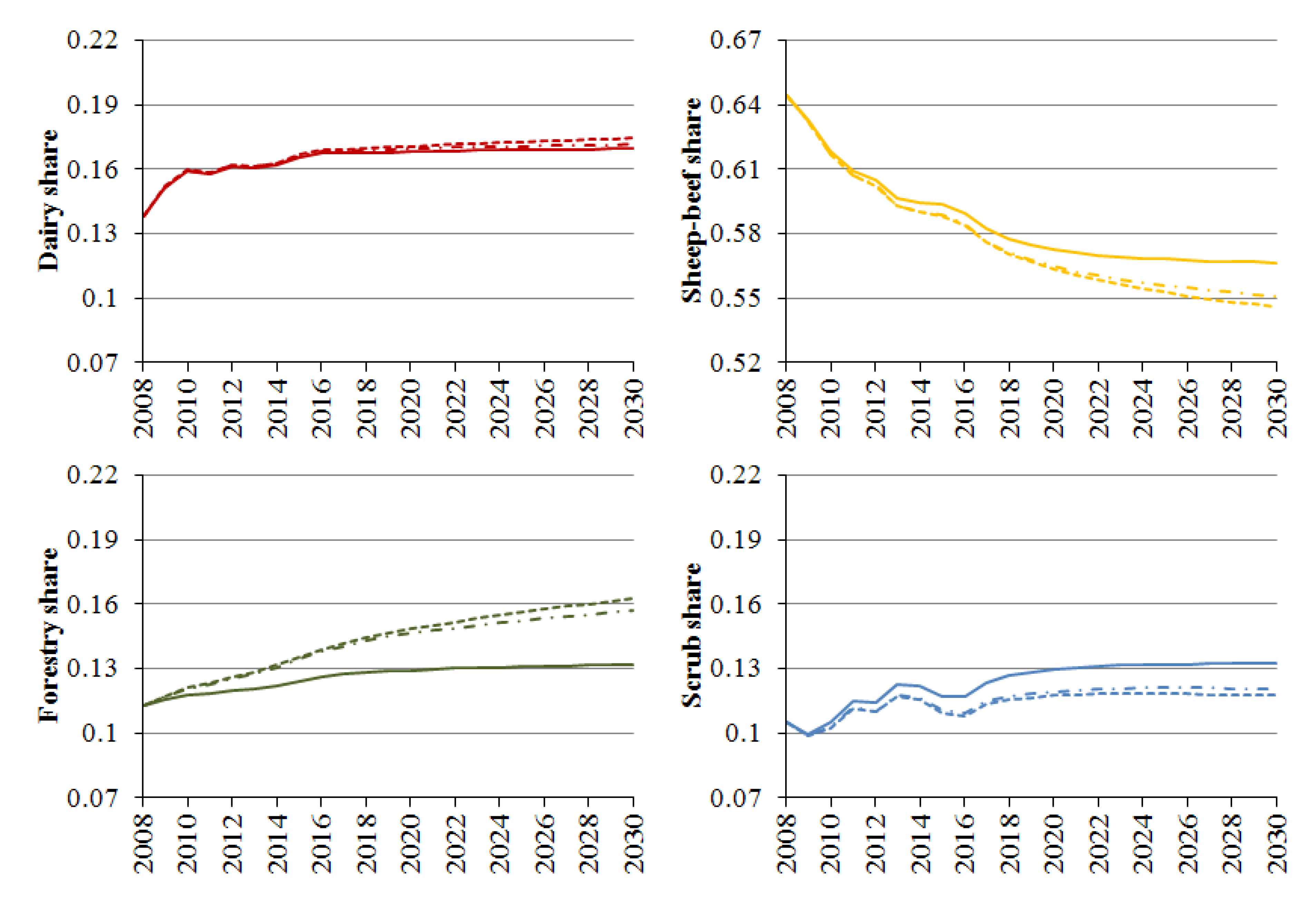
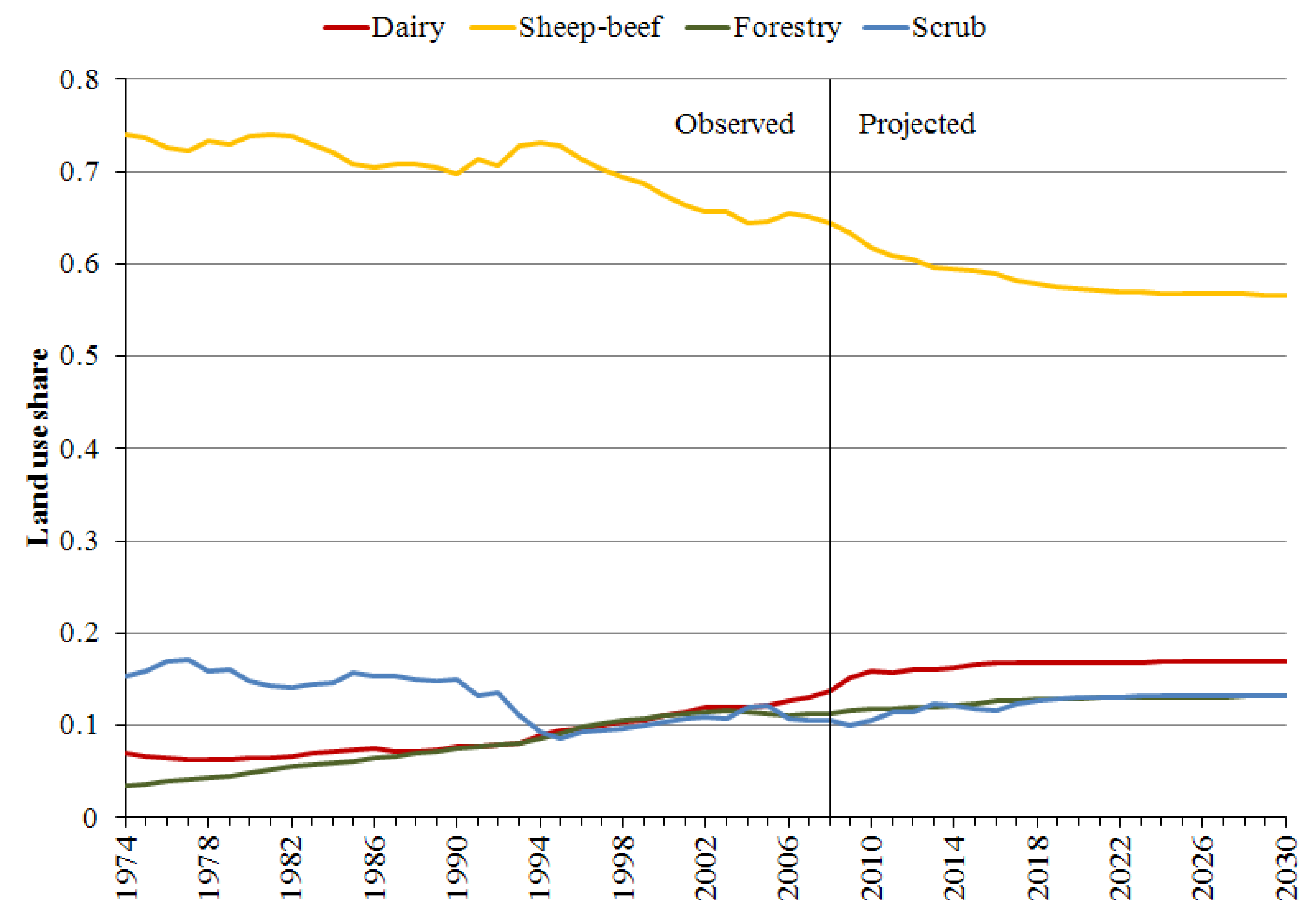
3.1. National-Level Land-Use Change

Figure 1 presents historical land use as well as baseline projections. The sheep-beef sector’s land share fell by nine percentage points in 14 years, from its peak of 73% of private rural land in 1994, to 64% in 2008. Even without any policy changes, we project the sheep-beef share to fall by a further seven percentage points, so that it will account for 57% of private rural land by 2030. The dairy land share has steadily increased in recent history. We project that this increase will continue, from 13.8% to 16.9% of rural land by 2030, under the baseline scenario. Forestry’s land share will rise, and we also project an increase in scrub. We interpret the increasing scrub share as abandoned sheep-beef land. As noted by Kerr and Olsen [11], our dynamic results for gradual land-use change are similar to those of Stavins and Jaffe [27] and consistent with Hornbeck [28].
The rise in plantation forestry area under the baseline scenario contradicts Adams and Turner [23], who project a decrease in forest area without an ETS. A potential explanation is offered by our different assumptions about future commodity prices (and hence the relative profitability of land uses). While Adams and Turner do not consider changes in commodity prices, we use official projections from the Situational Outlook for New Zealand Agriculture and Forestry (SONZAF), as explained in the appendix. Forestry log prices are projected to increase substantially by 2015, making forestry a relatively more attractive land-use choice in our model.
Figure 1. Baseline national-level land-use share projections, 2009–2030. Details on the projections are in the appendix.
Forests 03 01133 g001
Figure 2 focuses on the projected period and shows land-use shares by sector in each of the three scenarios. As expected, the ETS policies increase the amount of land in forestry and decrease the amount of land used for sheep-beef farming (mainly through conversions of marginal sheep-beef farms to forestry). Scrub land can earn a reward for sequestration by regenerating native forests under the ETS—we account for this reward in our land-use modeling, as explained in the appendix. Under both ETS scenarios, the total amount of land in scrub falls (as the decomposition in the next subsection makes clear, this is despite our projection that some marginal sheep-beef land is abandoned to scrub). The dairy share increases marginally in both ETS scenarios. The increase in dairy between the scenario with and without agriculture is plausible: when agriculture is included, it is possible that some high-quality sheep-beef farms convert to dairy, because, in percentage terms, the impact of the ETS on sheep-beef profits is larger than its impact on dairy profits [29].
Under the full ETS scenario and a carbon price of NZ$25, we project an increase of about 370,000 hectares in forestry area by 2030. Despite the large differences in our simulated baseline outcomes, this increase is very close to that projected by Adams and Turner for the same period under a slightly lower carbon price of NZ$20. Building on previous work by Horgan [30], Manley and Maclaren [31] also project a similar rate of net forest area increase—250,000 hectares by 2020—at a carbon price of NZ$25.
Figure 2. National land-use share projections by policy scenario, 2009–2030. Solid lines give baseline projections. Dash-dot lines give an ETS without agriculture. Dashed lines give the full ETS. Note that the y-axis does not extend to zero; however, the vertical spread of each y-axis is the same so that comparisons can be made across graphs.
Forests 03 01133 g002
There are two other important inferences to draw from Figure 2. First, in every sector the impact of including agriculture in the ETS is to magnify the effect that would have occurred without it (while the direction of the effects remains the same). However, having an ETS that rewards forest owners (and scrub owners) for sequestration has far larger impacts on land use than incrementally extending the ETS to also include agriculture. Second, in all sectors except forestry, the difference in land use across scenarios is smaller than the difference in land use across time within the baseline. Thus, while the LURNZ projections imply that the ETS matters for land-use decisions, its effect is relatively small in the context of wider changes in the economic environment [32].

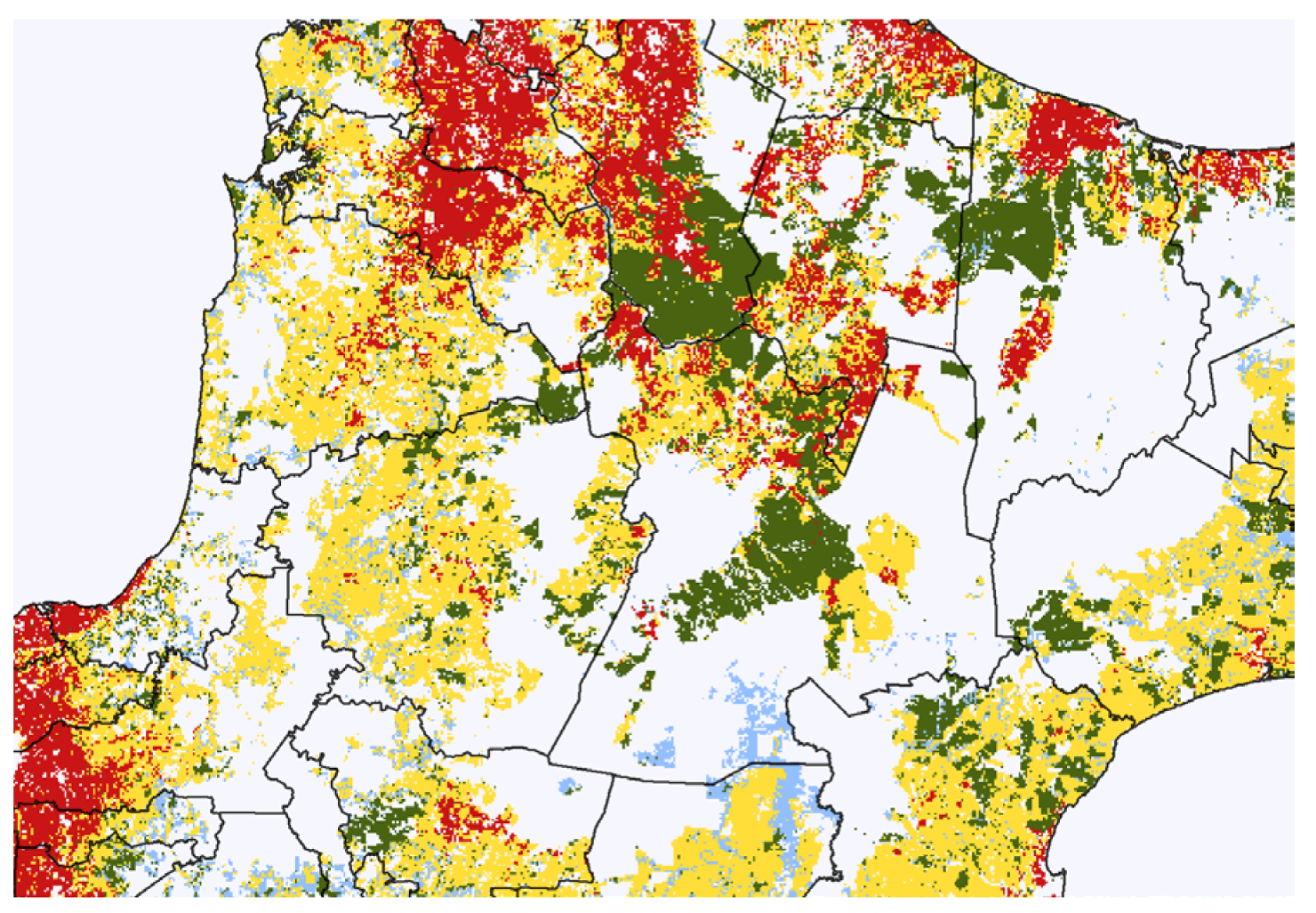
3.2. Regional Land-Use Change

Given the land-share projections presented in the previous section, the LURNZ model allocates land to different uses spatially for each year of the simulation. Figure 3 shows central North Island land use in the baseline scenario in 2030. This map illustrates the spatial resolution at which LURNZ makes projections.
Making use of the spatial mapping capability of LURNZ, Table 1 breaks down baseline land-use change in hectares over time by regional council (note that the amount of private rural land varies from council to council). For the Bay of Plenty region, for example, we project that 5725 hectares of sheep-beef land will convert to dairy, 12,225 hectares of sheep-beef land will convert to forestry and 5250 hectares of sheep-beef land will be abandoned to scrub by 2030. At the same time, we project that 1900 hectares of dairy land and 50 hectares of scrub will convert to sheep-beef land in this region by 2030. In general, most land-use change is projected to take place on sheep-beef land. Most of the increase in baseline dairy shown in Figure 1 comes from sheep-beef; large areas of marginal sheep-beef land also convert to forestry and scrub. Additional new forest planting takes place on scrub land.
Figure 3. Baseline land use in 2030. The figure shows baseline land-use projections for central North Island in 2030. Dairy land is red, sheep-beef land is yellow, forestry land is green and scrub land is blue. White land is exogenous in LURNZ.
Forests 03 01133 g003
Table 2 summarizes land-use results under the full ETS and the projected baseline in 2030 by regional council; the table shows land-use differences, and not transitions [33]. The net changes are the same as in Figure 2. Land-use responses are spatially heterogeneous and depend on the geophysical and other characteristics of the land in each region. We project the ETS to have an especially large effect on land use in Northland; 72,425 hectares of land that is scrub in the baseline is forestry in the full ETS, and 16,075 hectares of land that is sheep-beef in the baseline is scrub in the full ETS in this region. (Northland is projected to experience large land-use changes over time under the baseline scenario as well, as shown in Table 1.)
Table 3 shows land-use differences between the two ETS scenarios (with and without agriculture) in 2030. The spatial distribution of land uses is similar across the two policy scenarios. In general, forest area is larger in the full ETS than in the scenario without agriculture, due to forestry’s increased relative attractiveness under the full ETS.
Table 1. Land-use change (in hectares) between 2008 and 2030 under the projected baseline by regional council.
Baseline 2030DairySheep-beefForestryScrub
2008 land useDairySheep-beefForestryScrubDairySheep-beefForestryScrubDairySheep-beefForestryScrubDairySheep-beefForestryScrub
Northland152,43028,8002501,9750161,4300004,925140,1802,1750210,450088,000
Auckland56,35025,4251251,500095,275065002,95037,5501,375031,325029,675
Waikato481,95033,9751504,6508,775647,980060082517,700229,60021,850016,025078,275
Bay of Plenty92,0005,725252751,900127,78005017512,225139,75010,20005,250017,225
Gisborne2,1006,5752500264,63000021,625137,73010,350064,775085,050
Hawke’s Bay19,2759,75006,8503,225656,60004,3502510,275109,35012,17509,800064,500
Taranaki197,2004,875250200148,28003,55007524,15016,6750850042,125
Manawatu133,68057,3751501,7751,425964,28001752531,825112,05012,12510072,125081,875
Wellington33,30028,27501,2500278,280060006,47548,1254,025017,500097,250
West Coast76,77502501,25063,37507501251,25029,4507,4752522509,075
Canterbury201,98076,8004252,0501,5251,261,000014,100067593,4504,375021,5500197,480
Otago79,55026,775757,5507001,211,30003,750257,400111,6001,1757561,250060,900
Southland153,23059,1501001,1750600,55004,85002566,8251,95000029,425
Tasman24,4257,20006752,90071,27505,7002251,05070,8003,1750475030,450
Nelson32517500503,55002250257,05012502503,375
Marlborough10,9255,77502251,875206,15008000055,5503,10000077,900
New Zealand1,715,495376,6501,37529,95023,8256,761,735040,1501,425118,5001,413,210112,325200511,6250992,580
Notes: Each cell shows the difference in land use between 2008 and 2030 under the projected baseline. The data blocks (columns with titles in bold) represent projected baseline land use, and the four columns within each block represent 2008 land use. For example, the first data block (bold dairy) shows that in the Taranaki region, 197,200 hectares of the 2008 dairy land remain in dairy use by 2030 under the projected baseline. Projected conversions to dairy are shown in this block: 4875 hectares of sheep-beef land and 25 hectares of forestry land to change to dairy. The first columns of the next three data blocks represent conversion out of 2008 dairy: 200 hectares are projected to change to sheep-beef in Taranaki by 2030. The determination of national-level land use is described in the appendix. The algorithm that spatially allocates uses is described in Anastasiadis et al. [14]. The Manawatu row refers to the area administered by the Manawatu-Wanganui Regional Council.
Table 2. Land-use differences (in hectares) in 2030 between the projected baseline and the full ETS scenarios by regional council.
Full ETS 2030DairySheep-beefForestryScrub
Baseline 2030DairySheep-beefForestryScrubDairySheep-beefForestryScrubDairySheep-beefForestryScrubDairySheep-beefForestryScrub
Northland183,4501,650251,5250142,4300001,275147,25072,425016,0750224,500
Auckland83,4001,75000080,17500010,72541,87528,22503,275032,775
Waikato520,7306,950125500633,70000011,850269,85028,30004,850065,950
Bay of Plenty98,0251,82520000122,5000003,375162,1503,52502,025018,950
Gisborne8,700800000237,75000010,700169,70029,625015,3750120,200
Hawke’s Bay35,8751,9500500653,5500003,925131,83012,77504,750061,475
Taranaki202,100625000147,9000001,72540,90015,07501,775027,900
Manawatu192,9805,0507500917,68000028,725155,95042,225014,4250111,880
Wellington62,8252,950000259,9300006,82558,62520,47509,175094,275
West Coast76,8004752525063,4500001,30038,2751,875015007,425
Canterbury281,25011,8757517501,251,3000001,05098,4255,375012,4250213,480
Otago113,9507,825010001,187,2000008,575120,2007,075012,1750115,050
Southland213,65010,65003000592,38000060068,80015001,775028,975
Tasman32,3001,4250125074,4000002,22575,2506,92501,825023,875
Nelson500250003,550000757,200800017502,600
Marlborough16,925675000206,50000085058,6501,7500800076,150
New Zealand2,123,46056,5005252,35006,574,39500093,8001,644,930276,6000101,05001,225,460
Notes: Each cell shows the difference in land use between two scenarios: the projected baseline and the full ETS. The data blocks (columns with titles in bold) represent 2030 land use under the full ETS scenario, and the four columns within each block represent projected baseline land use. For example, the areas in the final row of the first block sum to 2,182,835 hectares; this is the projected area of national dairy land under the full ETS. The majority of this area—2,123,460 hectares—is in dairy use under the projected baseline as well. The remainder is either sheep-beef (56,500 hectares), forestry (525 hectares) or scrub (2,350 hectares) under the baseline. The determination of national-level land use is described in the appendix. The algorithm that spatially allocates uses is described in Anastasiadis et al. [14]. The Manawatu row refers to the area administered by the Manawatu-Wanganui Regional Council.
Table 3. Land-use differences (in hectares) in 2030 between the full ETS and an ETS without agriculture scenarios by regional council.
Full ETS 2030DairySheep-beefForestryScrub
ETS no ag 2030DairySheep-beefForestryScrubDairySheep-beefForestryScrubDairySheep-beefForestryScrubDairySheep-beefForestryScrub
Northland184,580775251,2750142,4300000198,43022,52503,0500237,530
Auckland84,0001,15000080,1750001,35075,9753,5000475035,575
Waikato524,9002,85075250633,7000002,650302,8304,52501,250069,550
Bay of Plenty99,12580012500122,500000625168,0503750500020,475
Gisborne9,000500000237,7500001,850203,9504,22502,1500133,430
Hawke’s Bay36,8251,0000500653,5300250500146,4001,6250450065,775
Taranaki202,330400000147,90000015055,9001,6500100029,575
Manawatu195,0003,0505000917,6800004,650216,7505,50002,2500124,050
Wellington63,9501,825000259,9300001,42581,0503,45001,5500101,900
West Coast77,150150250063,45000047540,62535002507,550
Canterbury285,6307,675255001,251,2000500275103,65092501,3000224,600
Otago117,0304,82502501,187,20002501,425133,2801,15001,7500125,480
Southland218,1006,27502250592,38000022569,30025075030,675
Tasman33,150675025074,40000062582,5001,275025025,675
Nelson52500003,550000257,9001500002,775
Marlborough17,250350000206,50000027560,8751000175076,775
New Zealand2,148,54532,3003251,67506,574,2750100016,5251,947,46551,350015,12501,311,390
Notes: Each cell shows the difference in land use between two scenarios: the full ETS and the ETS without agriculture. The data blocks (columns with titles in bold) represent 2030 land use under the full ETS scenario, and the four columns within each block represent land use under the ETS without agriculture scenario. For example, the data for Marlborough Regional Council indicate that scrub area is 76,875 hectares under the ETS without agriculture (the sum of areas in the scrub columns of each block), and 76,950 hectares under the full ETS (the sum of areas in the scrub block). Most of this land—76,775 hectares—is projected to be scrub under both scenarios; 175 hectares are sheep-beef under ETS without agriculture, but scrub under full ETS; and 100 hectares are scrub under ETS without agriculture, but forestry under full ETS. The determination of national-level land use is described in the appendix. The algorithm that spatially allocates uses is described in Anastasiadis et al. [14]. The Manawatu row refers to the area administered by the Manawatu-Wanganui Regional Council.

4. Agricultural Emissions

Projected 2030 agricultural emissions are about 0.25 gigagrams lower under the full ETS than they are under the baseline. Table 4 decomposes this reduction by land use. Land that is sheep-beef in the baseline but forestry or scrub in the full ETS scenario achieves a reduction in agricultural emissions under the policy. At the national level, the policy slightly increases dairy land share; the land on which conversions to dairy take place has higher emissions under the policy. Overall, the reduction in agricultural emissions corresponds to less than 1% of the 2008 inventory of agricultural emissions.
Agricultural emissions in the two ETS scenarios are very similar, because the increase in emissions from additional conversions to dairy under the full ETS approximately balances out the reduction achieved by additional conversions to forestry and scrub. That is, most of the reduction in sheep-beef emissions in Table 4 is achieved by rewarding forestry and scrub.
Table 4. Differences in agricultural emissions (in gigagrams of CO2-equivalent) decomposed by 2030 land use.
Baseline land use
Full ETS land useDairySheep-beefForestScrub
Dairy00.2320.004 a0.016 a
Sheep-beef0000
Forest0−0.24000
Scrub0−0.26300
Net0−0.2710.0040.016
a These values represent a modeling anomaly and do not have a meaningful interpretation. Notes: Differences in emissions between scenarios are all due to land-use change; there is no on-farm mitigation. Details about emissions calculations can be found in Timar [13].

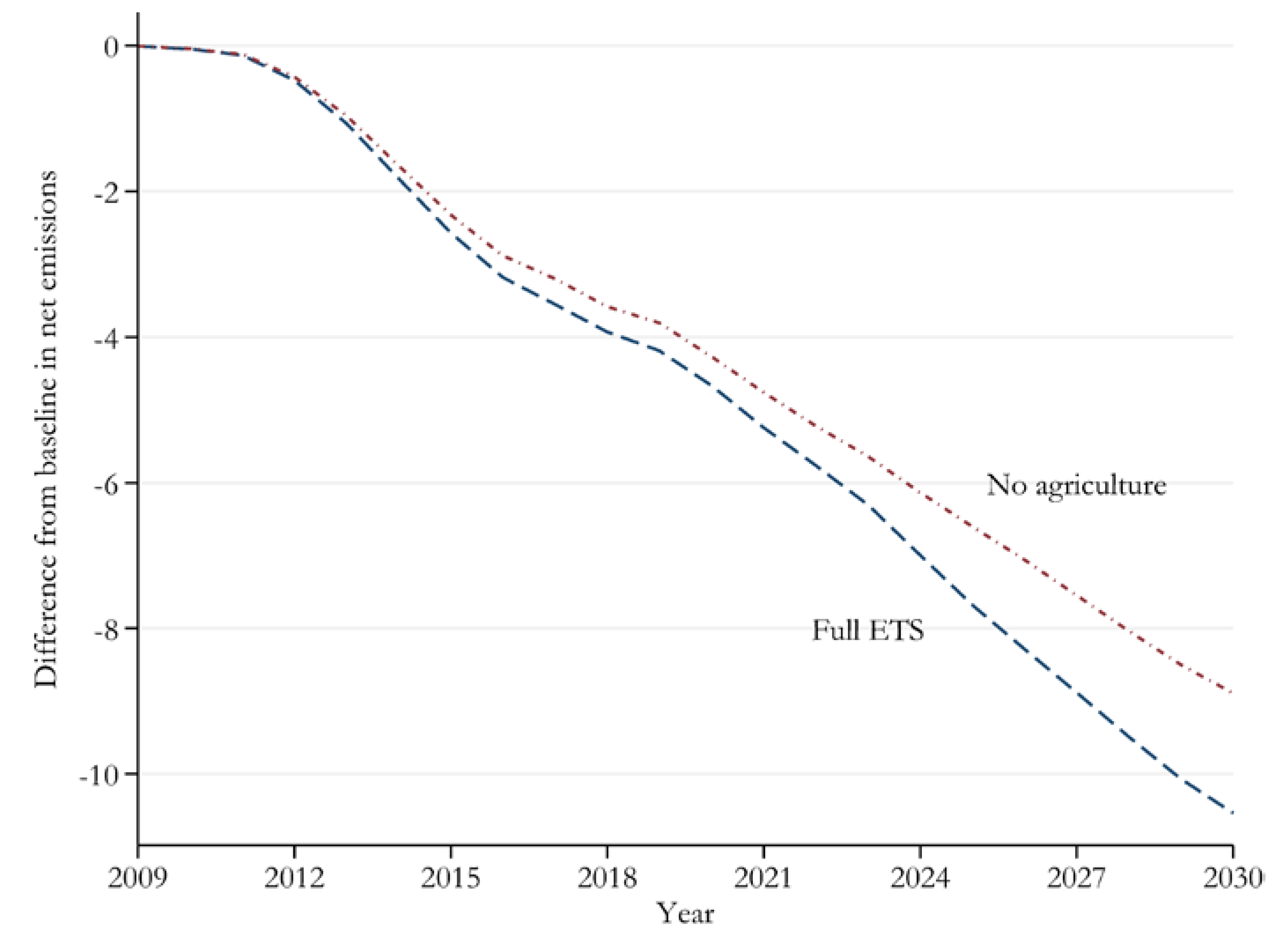
5. The Time Path of Policy-induced Net Forestry Emissions
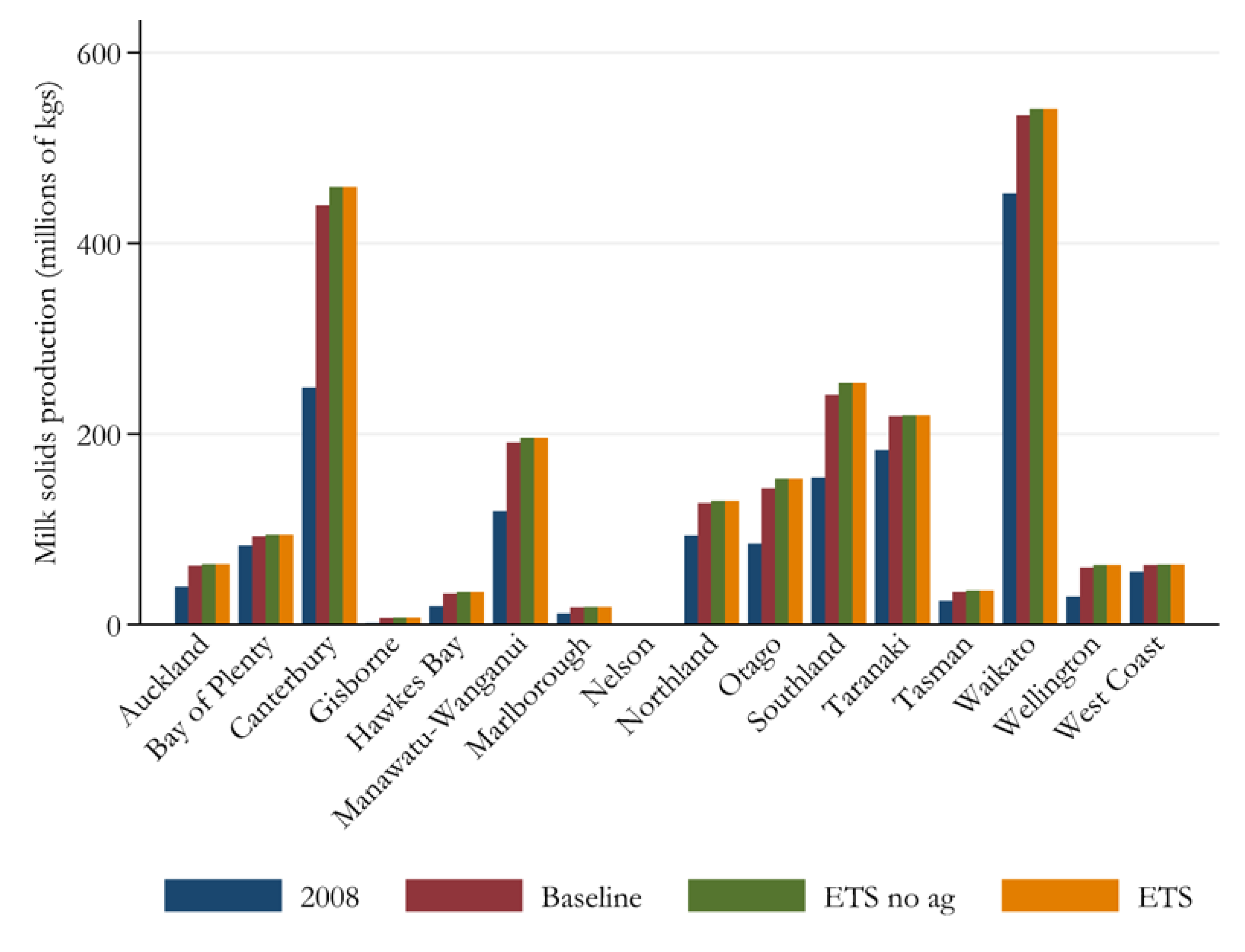
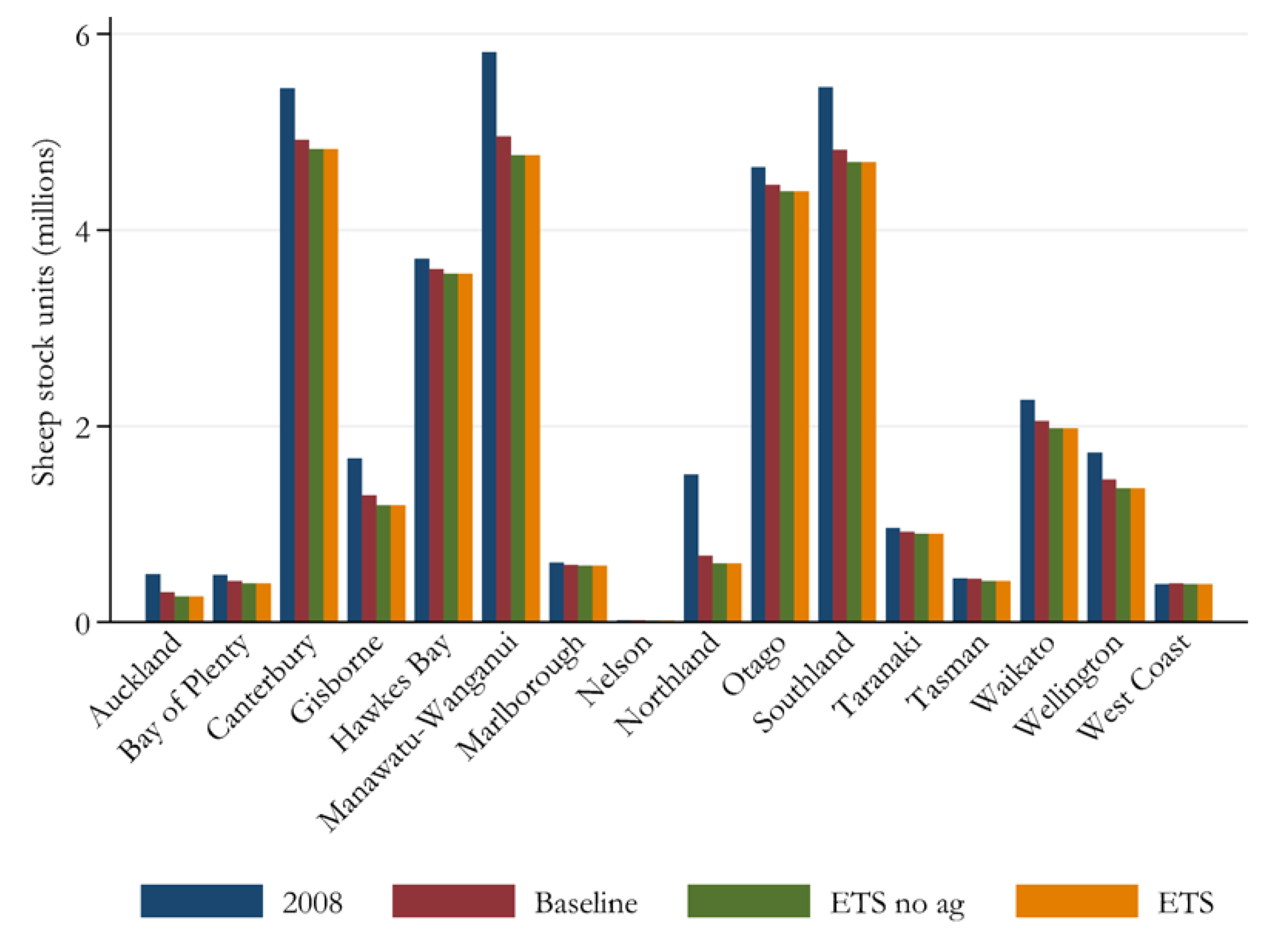
As forests grow, they remove carbon dioxide from the atmosphere through the process of carbon sequestration. In this section, we present projections on the difference in net carbon removals from private plantation forests in LURNZ between the baseline and each policy scenario, as illustrated by Figure 4. The difference in removals across scenarios is driven by the quantity, timing and location of afforestation since 2008. There are two reasons for this. First, deforestation is negligible in all three scenarios, and second, in 2008, the quantity, location and age distribution of forests are the same across all scenarios. Consequently, removals and emissions from New Zealand’s legacy of afforestation are the same across scenarios, except for new planting. In 2024 (at the expected peak of emissions from forestry), LURNZ projects that private forests sequester 7 megatonnes more carbon in the full ETS than in the baseline, and slightly over 6 megatonnes more carbon in the ETS without agriculture than in the baseline. These figures correspond to 17.6% and 20%, respectively, of New Zealand’s 2008 gross agricultural emissions. However, by the early 2040s, net forestry emissions under the policy scenarios become higher than under the baseline as new forests planted in response to the policy reach harvestable age.
Figure 4. Annual differences from baseline in the net flow of emissions from forestry (in gigagrams of CO2). All pre-1990 and post-1989 forest on private land is included.
Forests 03 01133 g004
Projections by Adams and Turner [23] suggest a substantially larger policy effect on net forest sequestration. Their difference from the baseline reaches a high of 40 gigagrams of CO2 by 2024 with a NZ$20 carbon price. It is difficult to explain such a large discrepancy between our simulations, especially given the similarity in our overall forestry land area response to 2030. We attribute some of the difference to higher baseline deforestation rates brought about by relatively lower forestry returns in their simulations [34]. Because of this, some of the land-use response is achieved by decreased deforestation in their simulations, whereas it is almost entirely due to afforestation in our simulations. This leads to very different net emissions outcomes as the carbon released at harvest (and deforestation) is sequestered gradually over a period of 25–30 years. Agents’ carbon price expectations also play a large role in deforestation and afforestation decisions in Adams and Turner; we do not model multiple price expectations. Finally, the endogenous rotation length of their model may also contribute to the difference in our simulations by changing the timing of harvest decisions under the policy scenarios.
New Zealand’s Fifth National Communication under the United Nations Framework Convention on Climate Change [35] projects a reduction of about 3.4 gigagrams of CO2 in net forestry emissions with the ETS (relative to the baseline) by 2020. This reduction is similar in magnitude to our projection for 2020 (and smaller than that of Adams and Turner for the same year), despite the assumption of a higher mean carbon price in the Fifth National Communication [36].

6. Production

LURNZ simulates land use at a fine spatial resolution, allowing us to examine rural production at a regional level. We are therefore able to look at the differential impacts by region of ETS policies on rural production. (In doing so, we do not account for potential climate change-induced increases in New Zealand’s pasture production [37,38]. Such an increase would affect both our baseline and policy scenarios and can be considered a second-order effect.) Because rural production affects local labor market opportunities and regional incomes, this is important in determining the regional welfare effects of the ETS.
Figure 5 shows projected milk solids production by regional council in 2030 under each policy scenario. We also present milk solids production by regional council in 2008 to serve as a reference point. Regional milk solids production in 2030 depends on the amount of dairy land in the region, as well as on estimated increases in dairy productivity between 2008 and 2030; productivity estimates in LURNZ are documented in Timar [13]. Canterbury, Manawatu-Wanganui, Southland and Taranaki regional councils all increase milk solids production substantially within the baseline. However, it is clear from the graphs that milk solids production does not change much across policy scenarios, because dairy land use does not respond strongly to the ETS.
Figure 5. Milk solids production by region in 2008 and in 2030 policy scenarios. Blue bars show LURNZ estimates of the total output by regional council in 2008. Red, green and orange bars show, respectively, projected output in 2030 under the baseline, with an ETS that does not include agriculture, and under the full ETS. Details on output projections are in Timar [13].
Forests 03 01133 g005
Figure 6 and Figure 7 show projected sheep and beef stock units by regional council in 2030 under each policy scenario. Once again, differences within the baseline are larger than differences across scenarios; recall from Figure 2 that the change in the sheep-beef land share within the baseline is also larger than the change across scenarios. There are reductions in sheep stock units and beef stock units in most regional councils. Northland and Manawatu-Wanganui are both projected to reduce sheep and beef stock units, and this is consistent with these regional councils having relatively more land in forestry and scrub compared to in sheep-beef under the ETS scenarios.
At the national level, the full ETS causes a reduction in sheep-beef land area by 3.7% and an overall reduction in sheep and beef stock units by 3.6% relative to the baseline. The reduction in stock units is relatively smaller than the reduction in land area, because the land that converts to another use has, on average, a lower carrying capacity.
Figure 6. Sheep stock units by region in 2008 and in 2030 policy scenarios. Blue bars show LURNZ estimates of the total stock units by regional council in 2008. Red, green and orange bars show, respectively, projected output in 2030 under the baseline, with an ETS that does not include agriculture, and under the full ETS. Details on stock unit projections are in Timar [13].
Forests 03 01133 g006
Figure 7. Beef stock units by region in 2008 and in 2030 policy scenarios. Blue bars show LURNZ estimates of the total stock units by regional council in 2008. Red, green and orange bars show, respectively, projected output in 2030 under the baseline, with an ETS that does not include agriculture, and under the full ETS. Details on stock unit projections are in Timar [13].
Forests 03 01133 g007

7. Conclusions

Motu has developed an integrated model, LURNZ, to study land-use change and associated environmental issues. In this paper, we have compared two different ETS scenarios with a baseline scenario using this simulation model. We project land-use change and consequent emissions and production changes across policy scenarios. Simulated land-use change under our baseline is driven by historical land-use dynamics and commodity price projections. This highlights the fact that the economic environment that is not directly related to the ETS is also crucial to future land-use decisions. In both policy scenarios, the simulated land-use responses occur gradually over time, suggesting that it may take several years before the full impact of ETS policy becomes apparent.
We project that in every ETS scenario, forestry land area increases relative to the baseline and sheep-beef land area falls. Associated with this land-use response, the sheep-beef sector’s contribution to national agricultural emissions falls under each scenario. On the other hand, when sheep-beef and dairy are both included in the ETS, we project that some land will convert from sheep-beef to dairy, increasing the contribution that dairy farming makes to New Zealand’s total emissions. Production is affected in the same direction as land use, but to a relatively smaller extent (for sheep-beef farming), because the land-use response takes place on marginal land.
Under our ETS scenarios, there is substantial reforestation. At a NZ$25 carbon price, the extra removals associated with this new planting mean that the additional sequestration in 2024 is projected to reach 17.6%–20% of the 2008 national inventory agricultural emissions. Thus, LURNZ simulations suggest that the ETS has considerable ability to reduce the liabilities that New Zealand will face when a significant number of post-1989 forests reach harvestable age.
Our simulation model also lets us evaluate the relative importance of including agriculture in the ETS. The results suggest that if forestry is rewarded for sequestration, the additional effect of bringing agriculture into the ETS is small in terms of both land-use change and net emissions reduction. This is despite the fact that in our full ETS scenario, agricultural participants are fully liable for their emissions. Including the free allocation of NZUs to the sector would reinforce our finding by further reducing the simulated response to the agriculture component of the ETS.
The projected reduction in net emissions reflects only the land-use response, as we do not model on-farm mitigation. This is consistent with the current agriculture ETS legislation placing the point of obligation at the processor level. Such a system simply amounts to raising costs in proportion to average national emissions within each sector, and therefore, it provides little incentive for on-farm mitigation. It is not clear how placing the point of obligation at the farm level would affect our results. On the one hand, the additional mitigation options could enable farmers to reduce their emissions liabilities without changing their land use, potentially reducing the size of the land-use response even further. On the other hand, many on-farm mitigation technologies are most effective (and feasible) on dairy farms, and could thus encourage additional dairy conversions from sheep-beef, potentially raising overall emissions.
The scale of the simulated land-use response is sensitive to parameter estimates from our dynamic land-use share model and to particular modeling assumptions we make in implementing LURNZ. For example, our results greatly depend on how we model the value of carbon credits to plantation forestry and on our assumptions about how carbon costs feed through to commodity prices.
There are currently few economic analyses of the New Zealand ETS that provide quantitative national-level land-use projections directly comparable to ours. While observations appear to indicate that the initial land-use response to the forestry ETS is smaller than our simulated land-use response, this may be explained by the policy uncertainty surrounding the ETS and the current low international carbon price.

Appendix on National Land-use Modeling in LURNZ
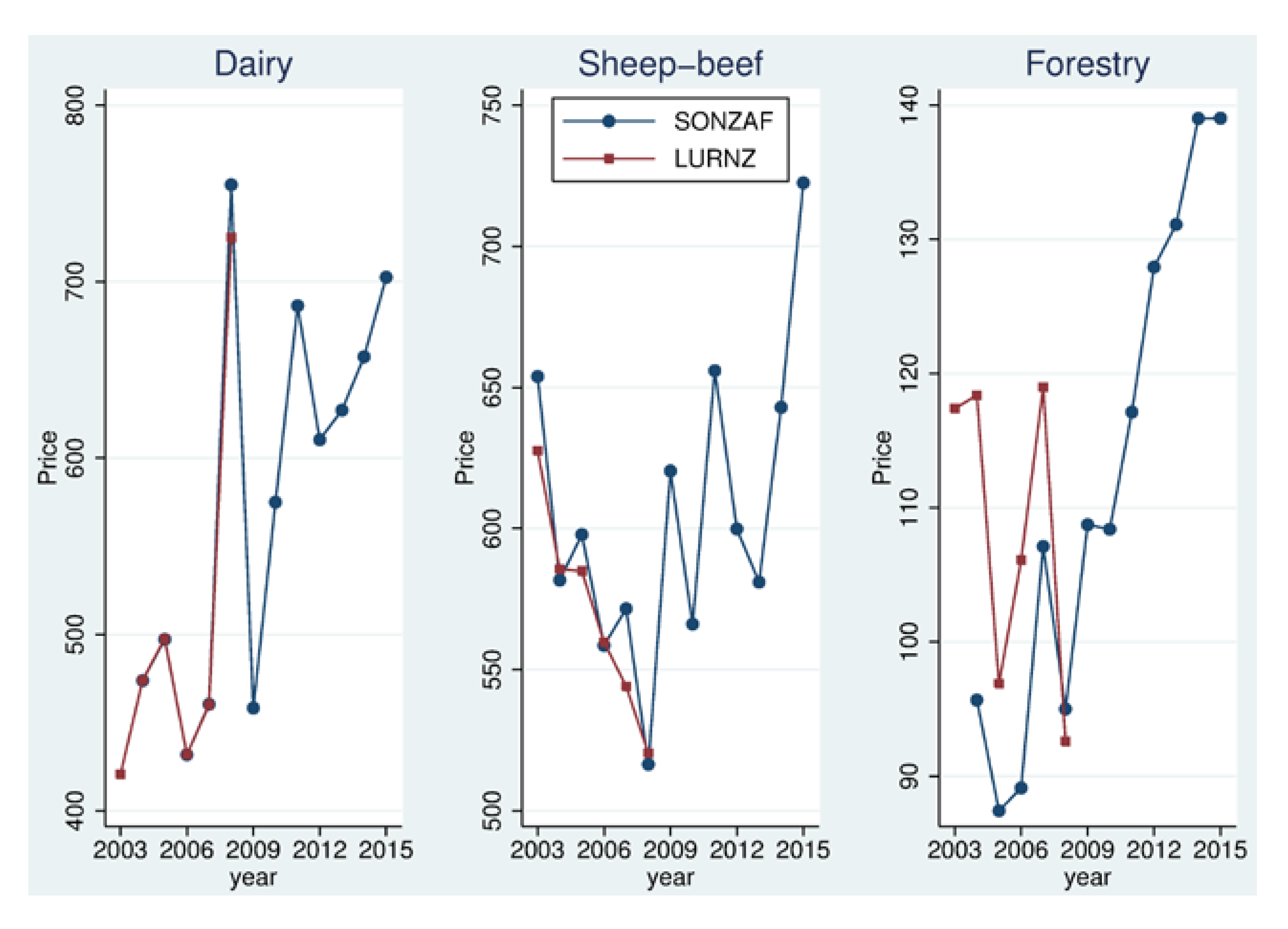
In this appendix we discuss a number of decisions that we made in calculating our land-use projections. First, we need to make some assumptions about future commodity prices and interest rates, as these are key explanatory variables used to estimate changes in land-use shares. Second, in order to model the effect of various carbon prices, we must make some assumptions about how carbon prices feed through to commodity prices. This is because we have estimates of the effects of commodity prices on land-use shares, but clearly we cannot have direct estimates of the effects of carbon prices on land-use shares. We also discuss modeling decisions we felt were necessary to make the projections more reasonable.

Price Projections

The coefficients of the dynamic econometric model are estimated using historical commodity prices [11]. Milk solids prices are reported in the Livestock Improvement Corporation’s (LIC) Dairy Statistics reports; the sheep-beef price is a composite export unit value calculated from New Zealand’s Overseas Merchandise Trade data set; forestry log prices are export unit values that match MAF’s values for logs and poles for every year that they report data. For simulations of future periods, we use commodity price projections provided by MAF’s Situational Outlook for New Zealand Agriculture and Forestry (SONZAF). Figure A1 presents the price series used in the econometric estimation of price responsiveness, as well as the observed and projected SONZAF prices. We do not use historical SONZAF prices in estimation because they are available for only a short period of time. We justify our use of SONZAF price projections for creating future projections of land use by noting that the corresponding historical portions of the series are reasonably consistent (though the match is not perfect for forestry). SONZAF projections are available until 2015; for subsequent simulation years we hold each price constant at its 2015 value: this would be our best estimate of its future value if we modeled prices as random walks.

Modeling the Impact of Carbon Prices

We now discuss how we convert carbon prices into changes in the commodity prices that are used to model land-use change. We assume that carbon costs affect farm decision-making in exactly the same way as commodity prices do through their effect on profits. Incidence of costs between the dairy and sheep-beef sectors is not clear, and we make several simplifying assumptions.
For dairy and sheep-beef we model the effect of carbon prices on commodity prices by using MAF’s 2012 emissions factors [39], dairy statistics from LIC, and detailed data on slaughter weight and animal numbers from Statistics New Zealand (SNZ). This enables us to calculate kilograms of CO2-equivalent greenhouse gas emissions per kilogram of milk solids and meat; we assume these stay constant over time. What remains is to add in the component of emissions from fertilizer. We do not have data on the average amount of fertilizer used per kilogram of milk solids or sheep-beef meat composite, so we use data from the national inventory.
Figure A1. A comparison of observed prices as used in the econometric estimation of price responsiveness (LURNZ) and as reported by SONZAF, as well as SONZAF price projections.
Forests 03 01133 g008
Some example calculations will make things concrete. To calculate the kilograms of emissions per kilogram of milk solids we proceed as follows. First, we calculate the median lifespan of a cow using LIC data on survival rates. This gives us a median life span of 6.31 years. We assume that a cow is milked for every year beyond its first; this gives us median milking years per cow to be 5.31 years. Multiplying this by 323 (the average number of milk solids per cow) and 6.14 (the MAF emissions factor for dairy milk solids), we get an estimate of the amount of lifetime emissions from a cow, which is 10,554 kilograms of CO2-equivalent. In 2008, SNZ reported that the mean average carcass weight for cows was 203.73 kilograms. This allows us to estimate the amount of emissions associated with the slaughter of a cow. We multiply 203.73 by 7.9 (the MAF emissions factor for cow carcass weight) and add 1980 (the MAF emissions factor per cow head). This gives us total emissions per cow of 14,133.52 kilograms in CO2-equivalent. Dividing this by the estimated amount of milk solids a cow produces over its lifetime, we calculate emissions per kilogram of milk solid as 8.23 kilograms of CO2-equivalent. This number does not yet account for fertilizer-related emissions.
To calculate sheep-beef emissions, we use the appropriate MAF emission factor for each category of meat for which SNZ provides slaughter data. For example, we use a carcass weight of 16.47 kilograms per lamb. Multiplying this by 4.5 (the MAF emissions factor per kilogram of meat) and adding 300 (the MAF emissions factor per head), and then dividing by the total amount of meat per lamb, we estimate that the emissions per kilogram of lamb meat (excluding fertilizer) are 22.71 kilograms of CO2-equivalent.
We also account for fertilizer emissions. To determine the average fertilizer intensity (in kilograms of nitrogen per hectare) on dairy and sheep-beef land, we turn to the 2007 Agricultural Census [13]. Using estimates of average output per hectare, we calculate an estimate of fertilizer-related emissions per output: 0.58 kilograms of CO2-equivalent per kilogram of milk solids and 0.52 kilograms of CO2-equivalent per kilogram of sheep-beef meat. We add these to the appropriate livestock-related emissions.
Afforestation decisions have historically depended on anticipated timber returns at harvest time; we use forestry log prices as a proxy. Under the ETS, forests can also make a carbon return. In order to model the impact of the ETS on the amount of land used in forestry, it is necessary to model the return to carbon forestry (and to translate this return into a log price-equivalent effect). However, capitalizing on the carbon return can expose landowners to two types of risk. The first is a price risk: landowners who opt into the ETS and sell their carbon credits as they receive them could face large liabilities at harvest time if the carbon price has increased sufficiently. This risk is potentially less relevant to large forest owners, who can stagger harvest times or develop forests with equal age distributions so that sequestration in each year offsets harvest liabilities [10]. The second type of risk has to do with policy uncertainty around the ETS, and arises in the years when owners are selling credits. It is possible that the scheme could be removed (or the value of credits could fall dramatically); forest owners would then receive little or no return for sequestration.
We model the carbon return to plantation forestry as the net present value of carbon credits from the first 10 years of forest growth using constant real carbon prices. Land managers’ actual valuations of carbon return depend on idiosyncratic parameters that are difficult to model; these include parameters for risk aversion, as well as expectations over future carbon prices, which may depend heavily on expectations over future policy. However, there is an important way in which using the net present value of carbon credits from the first 10 years provides a conservative valuation. The carbon stock at 10 years coincides with the minimum carbon stock held on land that is always replanted; thus, there is no liability risk from selling the carbon credits accumulated during the first 10 years. Of course, the value of those credits still depends on carbon prices and policy.
We perform the net present value calculations using the unweighted average of regional carbon stock from MAF look-up tables [19], a constant carbon price, and a real discount rate of 8%. The net present value thus represents the amount of money for which a forest owner could sell the future rights to the credits (to a buyer with an 8% discount rate). If the forest owner deposited this money in the bank, it could earn a risk-free return, which we assume to be 5 percent [40]. Because timber returns are realized at harvest time, we convert the net present value of the carbon return to a future return using the risk-free 5% rate. This is the value we add to our projected forestry prices to account for the value of sequestration credits earned.
Finally, under the ETS scrub land can earn a return for its sequestration. There are no data on historical responses to scrub returns, as scrub did not earn a monetary return before the ETS. We model scrub returns through changing the value of the outside option in other land uses. The carbon return from sequestration increases incentives for land to be used as plantation forestry, but the fact that carbon returns can be earned from regenerative scrub reduces this incentive; the potential for carbon returns on scrub compounds the disincentive from agricultural carbon costs. Thus, we further adjust each of our projected price series to reflect the fact that the value of the outside option has changed. In particular, we subtract the potential carbon reward to scrub from the (already adjusted) price projections.
We calculate the scrub carbon return in a manner identical to the method we use for determining the forestry carbon return: we use only the first 10 years of credits [41]. We annualize the net present value of these credits and subtract the result from the agricultural price projections. As forestry decisions depend on anticipated returns at harvest, we find the appropriate future value of the carbon return to scrub using the money interest rate; this is the value we use to adjust forestry price projections. The adjusted commodity prices and the nominal interest rate used for the various scenarios in LURNZ simulations are shown in Table A1.
Table A1. Adjusted commodity prices and the five-year nominal interest rate as observed in 2008 and as used in LURNZ simulations (from 2009).
YearDairy priceSheep-beef priceForestry priceInt. rate
BLETS 1ETS 2BLETS 1ETS 2BLETS 1ETS 2All
2008725.0721.9721.9520.4490.1490.192.6109.1109.16.17
2009458.3455.1455.1620.5590.2590.2108.7125.3125.33.70
2010580.6577.5577.5571.7541.5541.5109.5126.0126.02.70
2011683.1680.0680.0652.9622.6622.6116.6133.1133.13.00
2012606.9603.8603.8596.5566.2566.2127.2143.8143.83.00
2013627.2624.1624.1581.1550.9550.9131.1147.7147.73.90
2014660.7657.6638.2646.2616.0562.5139.7156.3156.34.70
2015708.8705.7686.4729.0698.8645.1140.3156.8156.85.00
Notes: “BL” represents the baseline scenario, “ETS 1” is ETS without agriculture and “ETS 2” is the full ETS scenario. The units for dairy, sheep-beef and forestry prices are as follows: cents per kilogram of milk solids, cents per unit composite of sheep-beef output and dollars per cubic meter of wood. The interest rate does not vary across scenarios. SONZAF price projections are available until 2015; for subsequent simulation years we hold all prices and the interest rate constant at their 2015 levels.

Modeling Decisions

Dairy share is handled specially in LURNZ. One uncomfortable result in the dynamic land-use model is that in every specification we estimated, the share of land in dairy farming increases when forestry export prices increase. We attribute this result to the fact that our national analysis has little data with which to work, and do not think that it represents a causal relationship. If we did not do anything about this relationship, most of the change from baseline in our dairy share projections would be driven by the ETS effect on forestry returns. We do not think this is reasonable. Thus we calibrate our projections. In particular, we run an auxiliary scenario in which we do not let forestry prices change in response to the ETS. The change in dairy share in this scenario is therefore not driven by changing forestry prices. We use this as our dairy share for our final scenario; for the other land uses we use their shares with the full ETS scenario, plus a third of the difference from dairy calibration added to each land use, to ensure that the adding-up constraint is met.
Finally, different carbon price scenarios result in different dynamics. We linearize the dynamics in the first 10 years to focus on the long-term pattern.

Conflict of Interest

The authors declare no conflict of interest.

Acknowledgements

This research has been funded by the Ministry of Science and Innovation through the Motu-led Integrated Economics of Climate Change programme, and by the Ministry for Primary Industries’ Sustainable Land Management Mitigation and Adaptation to Climate Change Programme through the Motu-led Coordination and Cooperation for Effective Climate Policy Design and Implementation grant. We thank staff at the Ministry for the Environment (MfE) and Ministry of Primary Industries (MPI), who have assisted with the interpretation of agricultural emissions data, staff at Beef and Lamb and DairyNZ who assisted with details on their sectors and Steve Wakelin and colleagues at Scion, who assisted with details of forestry sector modeling. We are grateful for comments received from participants in the EcoClimate consortium, at New Zealand Agricultural and Resource Economics Society conferences, at various research workshops and from two anonymous referees. All errors, omissions and judgments are those of the authors.

References and Notes

  1. Anastasiadis, S.; Kerr, S. Mitigation and heterogeneity in management practices on New Zealand dairy farms. Unpublished manuscript.
  2. Jiang, N.; Sharp, B.; Sheng, M. New Zealand’s emissions trading scheme. New Zeal. Econ. Papers 2009, 43, 69–79. [Google Scholar] [CrossRef]
  3. Bertram, G.; Terry, S. The Carbon Challenge: New Zealand’s Emissions Trading Scheme; Bridget Williams Books: Wellington, New Zealand, 2010. [Google Scholar]
  4. Agriculture’s entry has been deferred by an amendment to ETS legislation passed in November 2012. There has been no change to the mandatory reporting requirement of agricultural emissions, which started at the beginning of 2012. All other sectors of the economy have either already entered the ETS in 2010 or are scheduled to enter it in 2013.
  5. Indigenous forests are protected in New Zealand and can almost never be logged.
  6. Karpas, E.; Kerr, S. Preliminary Evidence on Responses to the New Zealand Forestry Emissions Trading Scheme; Motu Working Paper 11-09. 2010. Available online: http://motu-www.motu.org.nz/wpapers/11_09.pdf (accessed on 25 September 2012).
  7. Ministry of Agriculture and Forestry. A Guide to Reporting for Agricultural Activities under the New Zealand Emissions Trading Scheme. 2011. Available online: http://www.mpi.govt.nz/news-resources/publications (accessed on 25 September 2012).
  8. To facilitate this comparison, we do not include a free allocation to agriculture in our full ETS scenario. Agricultural participants are therefore liable for all of their emissions starting from 2015 in our scenario.
  9. Manley, B.; Maclaren, P. Potential impact of carbon trading on forest management in New Zealand. For. Policy Econ. 2012, 24, 34–40. [Google Scholar]
  10. Turner, J.A.; West, G.; Dungey, H.; Wakelin, S.; Maclaren, P.; Adams, T.; Silcock, P. Managing New Zealand Planted Forests for Carbon: A Review of Selected Management Scenarios and Identification of Knowledge Gaps; Scion Ltd. Report; Ministry of Agriculture and Forestry: Wellington, New Zealand, 2008. Available online: http://www.mpi.govt.nz/news-resources/publications (accessed on 25 September 2012).
  11. Kerr, S.; Olssen, A. Gradual Land-Use Change in New Zealand: Results from a Dynamic Econometric Model; Motu Working Paper 12-06. 2012. Available online: http://motu-www.motu.org.nz/wpapers/12_06.pdf (accessed on 20 July 2012).
  12. Timar, L. Rural Land Use and Land Tenure in New Zealand; Motu Working Paper 11-11. 2011. Available online: http://motu-www.motu.org.nz/wpapers/11_13.pdf (accessed on 20 July 2012).
  13. Timar, L. Land-use intensity and greenhouse gas emissions in the LURNZ model. Unpublished manuscript.
  14. Anastasiadis, S.; Zhang, W.; Power, W; Kerr, S. Derivation of land use maps from 2002 to 2008. Unpublished manuscript.
  15. Hendy, J.; Kerr, S.; Baisden, T. The Land Use in Rural New Zealand Model Version 1 (LURNZv1): Model Description; Motu Working Paper 07-07. 2007. Available online: http://motu-www.motu.org.nz/wpapers/07_07.pdf (accessed on 20 July 2012).
  16. Pfaff, A.; Kerr, S.; Cavatassi, R.; Davis, B.; Lipper, L.; Sanchez, A.; Timmins, J. Effects of Poverty on Deforestation: Distinguishing Behaviour from Location. In Economics of Poverty, the Environment and Natural Resource Use; Dellink, R.B., Ruijs, A., Eds.; Wageningen University, Environmental Economics and Natural Resources Group: Wageningen, the Netherlands, 2008. [Google Scholar]
  17. Irwin, E.G.; Bockstael, N.E. Interacting agents, spatial externalities and the evolution of residential land use patterns. J. Econ. Geogr. 2002, 2, 31–54. [Google Scholar] [CrossRef]
  18. Lubowski, R.N.; Plantinga, A.J.; Stavins, R.N. What drives land-use change in the United States? A national analysis of landowner decisions. Land Econ. 2008, 84, 529–550. [Google Scholar]
  19. Ministry of Agriculture and Forestry. A Guide to Look-Up Tables for Forestry in the Emissions Trading Scheme. 2011. Available online: http://www.maf.govt.nz/portals/0/documents/forestry/forestry-ets/2011-ETS-look-up-tables-guide.pdf (accessed on 25 September 2012).
  20. Chomitz, K.M.; Gray, D.A. Roads, land use, and deforestation: A spatial model applied to Belize. World Bank Econ. Rev. 1996, 10, 487–512. [Google Scholar] [CrossRef]
  21. Nelson, G.C.; Harris, V.G.; Stone, S.W. Deforestation, land use, and property rights: Empirical evidence from Darién, Panama. Land Econ. 2001, 77, 187–205. [Google Scholar] [CrossRef]
  22. Stavins, R.N. The costs of carbon sequestration: A revealed-preference approach. Am. Econ. Rev. 1999, 89, 994–1009. [Google Scholar]
  23. Adams, T.; Turner, J.A. An investigation into the effects of an emissions trading scheme on forest management and land use in New Zealand. For. Policy Econ. 2012, 15, 78–90. [Google Scholar] [CrossRef]
  24. In Adams and Turner’s model, expected future returns in agriculture are based on observed land values. This is potentially problematic, as land values often include option value components and do not, therefore, necessarily equal discounted returns in the current land use.
  25. Sohngen, B.; Sedjo, R. Carbon sequestration in global forests under different carbon price regimes. Energ. J. 2006, 3, 109–126. [Google Scholar]
  26. Daigneault, A.; Greenhalgh, S.; Samarasinghe, O. Economic Impacts of GHG and Nutrient Reduction Policies in New Zealand: A Tale of Two Catchments. Proceedings of the AAEA Organised Symposium at the 56th Annual Australian Agricultural and Resource Economics Society Annual Meeting, Fremantle, Australia, 8–10 February 2012; Available online: http://ageconsearch.umn.edu/bitstream/124284/2/2012ACDaigneaultCP.pdf (accessed on 25 September 2012).
  27. Stavins, R.N.; Jaffe, A.B. Unintended impacts of public investments on private decisions: The depletion of forested wetlands. Am. Econ. Rev. 1990, 80, 337–352. [Google Scholar]
  28. Hornbeck, R. The Enduring Impact of the American Dust Bowl: Short and Long-Run Adjustments to Environmental Catastrophe; NBER Working Paper 15605; National Bureau of Economic Research: Cambridge, MA, USA, 2009. [Google Scholar]
  29. Kerr, S.; Zhang, W. Allocation of New Zealand Units within Agriculture in the New Zealand Emissions Trading System; Motu Working Paper 09-16. 2009. Available online: http://motu-www.motu.org.nz/wpapers/09_16.pdf (accessed on 20 July 2012).
  30. Horgan, G. Financial Returns and Forestry Planting Rates; MAF Policy. 2007. Available online: http://maxa.maf.govt.nz/climatechange/reports/returns/page.htm (accessed on 30 November 2012).
  31. Manley, B.; Maclaren, P. Modelling the impact of carbon trading legislation on New Zealand’s plantation estate. New Zeal. J. For. 2009, 54, 39–44. [Google Scholar]
  32. Our projected economic environment is taken from the Ministry of Agriculture and Forestry’s Situational Outlook for New Zealand Agriculture and Forestry (SONZAF). This is discussed in detail in the appendix.
  33. This is because a cell could be forest in 2030 under the baseline and scrub in 2030 under the full ETS, but it need not have ever converted from forest to scrub; there could have been a sheep-beef to forest conversion in the former case and a sheep-beef to scrub conversion in the latter.
  34. Our allocation algorithm may contribute to differences in our baseline deforestation figures. A certain amount of change in forestry area can be attained with different combinations of afforestation and deforestation. We allow for potential deforestation for the purpose of dairy conversion even if forestry’s overall land-use share increases. However, we are unable to estimate directly the amount of deforestation that results from a change in commodity prices, so projections for it are purely driven by our allocation algorithm.
  35. Ministry for the Environment. New Zealand’s Fifth National Communication under the United Nations Framework Convention on Climate Change; Ministry for the Environment: Wellington, New Zealand, 2009.
  36. The report’s policy scenario is based on the carbon price increasing from NZ$25 to NZ$50 by 2015.
  37. Kaye-Blake, W.; Greenhalgh, S.; Turner, J.; Holbek, E.; Sinclair, R.; Matunga, T.; Saunders, C. A Review of Research on Economic Impacts of Climate Change; Research Report 314; Lincoln University: Christchurch, New Zealand, 2009. [Google Scholar]
  38. Baisden, T.; Timar, L.; Keller, E.D.; Smeaton, D.; Clark, A.; Austin, D.; Power, W.; Zhang, W. New Zealand’s Pasture Production in 2020 and 2050; GNS Science Consultancy Report 2010/154; GNS Science: Lower Hutt, New Zealand, 2010. [Google Scholar]
  39. New Zealand Government. Agriculture in the New Zealand Emissions Trading Scheme. Available online: http://www.maf.govt.nz/portals/0/documents/agriculture/agri-ets/agets-emissions-factors.pdf (accessed on 20 July 2012).
  40. Eight percent is a common discount rate for forestry; it exceeds the risk-free interest rate of 5% because forestry is not a risk-free investment.
  41. We proceed in this way for two reasons. First, any policy uncertainty around the ETS would increase the probability that sequestration returns to scrub would not be realised. Valuing the sequestration returns for the first 10 years only can be thought of as accounting for policy uncertainty. Second, although scrub is unlikely to be harvested (and hence unlikely to face a carbon liability in the future), scrub land could also be used to establish a permanent forest. We therefore need a fair comparison to the carbon returns to forestry.

