Article

Spatial Distribution and Volume of Dead Wood in Unmanaged Caspian Beech (Fagus orientalis) Forests from Northern Iran

by
Beitollah Amanzadeh
1,
Khosro Sagheb-Talebi
2,
Bahman Sotoudeh Foumani
3,
Farhad Fadaie
4,
Jesús Julio Camarero
5,6 and
Juan Carlos Linares
7,*
1
Research Center of Agriculture and Natural Resources of Guilan Province, Km 10 Tehran Highway, Rasht 3394-41635, Iran
2
Research Institute of Forests and Rangelands, Tehran 13185-116, Iran
3
Young Researchers Club-Islamic Azad University-Rasht Branch, P.O. Box 1841, Rasht 41436-64965, Iran
4
Faculty of Natural Resources, University of Mazandaran, Pasdaran Street 47415, P.O. Box 416, Babolsar 41432-67973, Iran
5
ARAID, Instituto Pirenaico de Ecología (CSIC), Avda. Montañana 1005, Apdo. 202, Zaragoza 50192, Spain
6
Departamento de Ecologia, Universitat de Barcelona, Avda. Diagonal 645, Barcelona 08028, Spain
7
Departamento de Sistemas Físicos, Químicos y Naturales, Universidad Pablo de Olavide, Ctra. de Utrera km 1, Sevilla 41002, Spain
*
Author to whom correspondence should be addressed.
Forests 2013, 4(4), 751-765; https://doi.org/10.3390/f4040751
Submission received: 4 June 2013 / Revised: 3 September 2013 / Accepted: 4 September 2013 / Published: 26 September 2013

Abstract

:
Unmanaged forests are remnants of natural ecosystems that provide a basis for close-to-nature silvicultural research and applications. These forests have high amounts of dead wood, and although this material is being increasingly studied, the diversity of dead wood in terms of different diameters, decay stages, and spatial distribution patterns is as important as its volume for understanding forest dynamics. Here, we study natural forests in northern Iran to investigate the spatial distribution, decay stages, and volume of dead wood in unmanaged temperate forests at different developmental stages. Three stem-mapped sampling plots (100 m × 100 m) were established in uneven-aged stands dominated by Caspian beech (Fagus orientalis Lispsky). The total dead wood ranged from 37 to 119 m2 ha−1. Our results imply a spatial distribution shift from aggregation to randomness for dead trees in Caspian beech forest succession. We detected significant spatial interactions (attraction) between living and dead trees at short to medium spatial scales (1–20 m) in the plot with the earlier successional stage, suggesting that intra-specific competition is a prevailing force causing tree mortality at the stem-exclusion phase. By contrast, as trees become dominant with the mortality of other trees, the random tree-mortality pattern prevails. The spatial distribution and volume of dead wood may serve as a management target in near-to-natural Caspian beech forest. On the basis of our results, conservation-oriented management strategies should take into account the increasing amount of dead wood, particularly of large diameter in a late stage of decay.

1. Introduction

Recently, uneven-aged forest stands have received increasing attention [1,2,3,4]. Unmanaged forests are remnants of natural ecosystems, providing a basis for nature-based forest management, i.e., to use natural forest ecosystems as a model and to guide forest management [2]. Natural forests are characterized by high amounts of dead wood of different sizes in all stages of decay, as well as by the presence of old and hollow trees [5,6]. The amount of dead wood has been increasingly used in forest management as an indicator of well-preserved forests [7,8]. However, a large amount of dead wood is not the only important factor that ensures forest biodiversity and ecosystem functioning [9]. Also the diversity of dead wood in terms of different diameters, decay stages, and spatial distribution patterns is as important as its volume [10]. Spatial-pattern analysis is a common tool in forest ecology, used to infer important processes of tree population dynamics [11,12]. Thus, in the study of dead-wood characteristics, quantifying the spatial patterns of dead trees is fundamental to understanding the prevailing process causing tree mortality. For instance, in the absence of growth data, the analysis of the spatial patterns of observed tree mortality enable us to infer competitive interactions among trees within the stand [13], these constituting a fundamental ecological driver regulating growth, survival, and tree-species coexistence [14,15,16].
In temperate forests, fine-scale gap dynamics, based on the death of individual or small groups of trees, is the main natural disturbance [15,16], providing a continuous presence of dead wood of different sizes and decay categories over time [17,18,19]. Remnants of temperate Caspian beech forests (Fagus orientalis Lispsky) provide a view of forest-ecosystem not influenced by humans, offering a better understanding of tree-mortality patterns within natural forest dynamics [20,21]. In Caspian beech forests, in the absence of major disturbances such as fire, windthrow often opens gaps in the canopy where regeneration can proceed [20]. Thereafter, density-dependent competition drives species turnover as well as succession and is responsible for shaping the stand-level structure [21]. Therefore, understanding spatial distribution and the volume of dead wood in unmanaged Caspian beech forests provides a basis for characterizing forest structure and succession [22,23,24]. Moreover, understanding the spatial distribution and volume of dead wood provides key insights for conservation-oriented management applications, promoting biodiversity and different stand successional stages [2,6].
Despite dead wood has received increased attention in recent years, there is limited information on the spatial distribution and volume of dead wood [7,10]. In the present study, we focus on natural forests of Caspian beech from northern Iran; standing as well as fallen dead trees were measured since they constitute the dead-wood components most influenced by forest managers, who may choose to leave some areas with dead wood [24]. Our specific aim was to quantify dead-tree spatial patterns, dead-wood amount and decay stage at different developmental stages of unmanaged stands. We hypothesized that: (1) the spatial pattern of living and dead trees occupy small scales; and (2) the spatial pattern of dead trees tends to be more regular as the total volume of dead wood increases over succession. Our results should provide reliable information on contrasting forest-development stages, these data being useful for further silvicultural decisions.

2. Materials and Methods

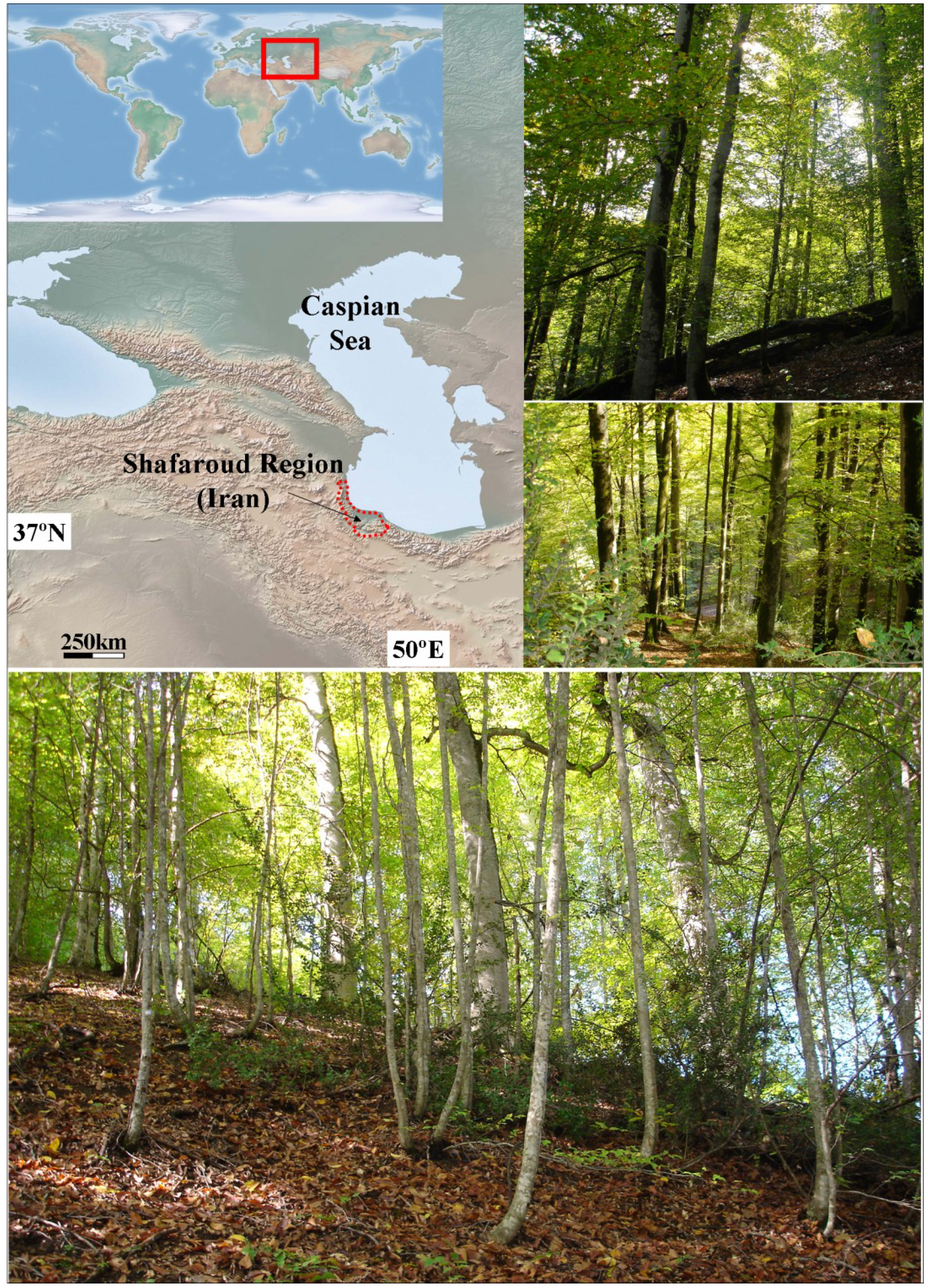
2.1. Study Site and Field Sampling

The study was conducted in an unmanaged forest within the Shafaroud region (northern Iran; 48º49′ E, 28º38′ N, 1200 m a.s.l. Figure 1). Parent material is igneous and metamorphic, mainly acidic. Well-drained brown forest soil is the dominant soil type and the slope ranges from 30% to 80%. Soils are deep, clay to clay-loamy in texture with acidic mull humus. The average annual temperature is 15.7 °C with maximum and minimum means of 21 °C and 10.5 °C, respectively. The mean annual precipitation is 990 mm with no significant dry period during the year. Irregular multi-aged Caspian beech (F. orientalis) was the dominant species associated with Persian Maple (Acer velutinum Boiss.), Cappadocian Maple (Acer cappadocicum Gled.), Hornbeams (Carpinus betulus L.) and Caucasian Alder (Alnus subcordata CAMey). The main species of forest floor were Euphorbia spp., Asperula spp., and Carex spp.
No silvicultural practice has been applied in this reserve area [21]. We performed an extensive field survey to select natural Caspian beech stands belonging to contrasting developmental stages. Three natural beech stands (1 ha in surface area; 100 m × 100 m stem-mapped sampling plot) were established. We studied standing live and dead trees with diameters greater than 7.5 cm, recording tree species, diameter at breast height (DBH) and location (X-Y coordinates); for fallen dead trees, we recorded the tree species, length, mid-diameter and rot rate. Fallen dead specimens were classified into decay classes as follows: recently fallen dead wood, rot class I; fallen dead wood with 25% decay, rot class II; fallen dead wood with 25%–50% decay, rot class III; fallen dead wood with >50% decay, rot class IV [25,26]. The volume of dead wood was estimated by the following equation:
Forests 04 00751 i001
where; d is the mid-diameter of the dead trunk and l is length of fallen dead tree. The volume of live and dead standing trees was measured using a Bitterlich relascope [15].
Figure 1. Geographical location of the study area (Shafaroud Region, northern Iran) and images of the study plots (Photographs take by B. Sotoudeh Foumani).
Forests 04 00751 g001

2.2. Point Pattern Analyses of Living and Dead Beech Trees
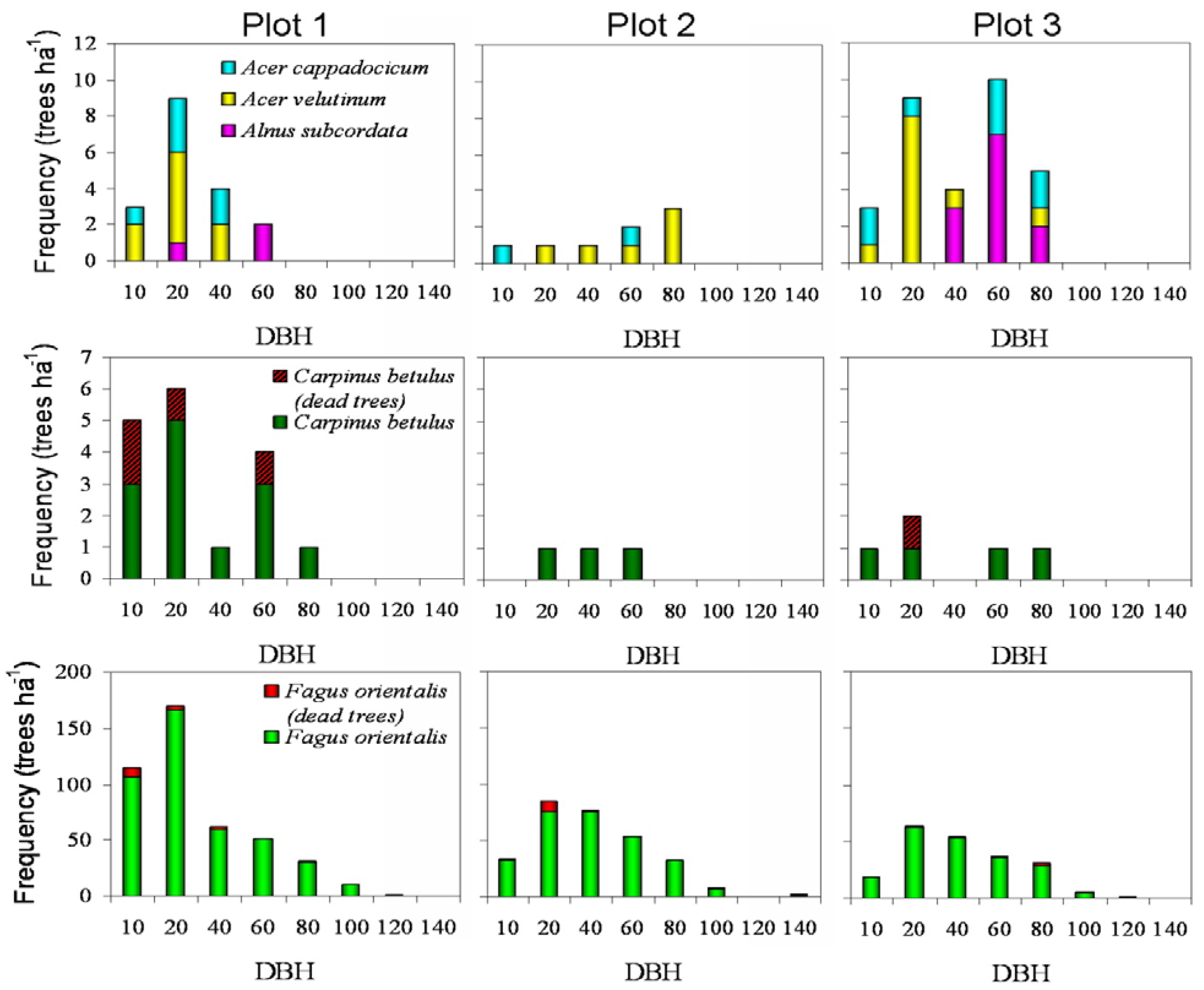
To analyze the spatial point patterns of living vs. dead beech trees, we used the bivariate g12(t) version of the pair-correlation function g(t) [11]. Values of g12(t) greater or less than 1 indicate attraction or repulsion, respectively. We carried out the spatial analyses up to 50 m (i.e., half the side of the plot) with a 1-m resolution. Because first-order effects due to environmental heterogeneity may mask second-order effects related to tree-to-tree spatial interactions, the selection of a null model is critical. First, we used the heterogeneous version of the g(t) to retain the large-scale structure of the pattern while removing local heterogeneity [27,28]. Second, we considered the random-labeling null model to investigate whether dead trees were randomly distributed within the combined pattern of dead and living trees [27].
This means that we assumed that tree death occurred throughout the plot independently of stochastic processes (e.g., recruitment) creating the coordinates of both living and dead trees (Figure 2). Finally, we compared the observed data with the upper or lower 95% bounds of the simulation envelopes based on 999 Monte Carlo simulations and also with the expected null model. The simultaneous testing of several distances may increase Type-I error, leading to the rejection of the null model even if it is true. Hence, we used a goodness-of-fit test (GoF) to summarize the total squared deviation between the observed pattern and the theoretical results across the distances analyzed in the univariate analyses [11]. Higher values of GoF indicate a stronger spatial pattern than lower values of GoF. Point-pattern spatial analyses were performed using the software Programita [29].
Figure 2. Frequency distribution of different tree diameters (diameter at breast height, DBH, cm) for three F. orientalis stem-mapped stands (plot 1, 2 and 3) from Shafaroud Region, northern Iran.
Forests 04 00751 g002

3. Results

3.1. Standing Dead Trees

A total of 475 trees with DBH of more than 7.5 cm were counted in the plot 1, including five tree species: F. orientalis, A. cappadocicum, A. velutinum, C. betulus, and A. subcordata (Table 1). In this plot, F. orientalis was the most frequent standing dead tree species, accounting for 16 individuals; C. betulus yielded four standing dead trees (Table 1, Figure 2). Overall, 4% of this plot was covered by dead trees, 80% belonged to F. orientalis, and the rest were C. betulus. In sampling plot 2, we recorded 303 trees, these being F. orientalis, A. cappadocicum, A. velutinum, and C. betulus. All standing dead trees belonged to F. orientalis (15 trees). In sampling plot 3, we counted 248 trees, with only 3% of the recorded trees standing. The most frequent standing dead tree was F. orientalis (86%), while C. betulus was also found (Table 1).
Table 1. Total number of living and standing dead trees recorded in the three study plots.
Living Trees
PlotF. orientalisA. velutinumA. subcordataC. betulusA. cappadocicumTotal
Tree Density142493136455
22776032288
(ind. ha−1)
3206111248241
Basal Area136.50.20.41.20.138.4
(m2 ha−1)234.71.400.20.136.5
327.50.62.50.51.232.3
Standing Dead Trees
PlotF. orientalisA. velutinumA. subcordataC. betulusA. cappadocicumTotal
Tree Density116004020
215000015
(ind. ha−1)
3600107
Basal Area10.8000.301.1
22.300002.3
(m2 ha−1)
31.800001.8
The DBH of standing dead trees varied among plots (Figure 2), suggesting different stand development stages. Although the number of standing dead trees was higher in the plots 1 and 2, large trees were more frequent in the plot 3. In both plot 1 and 2, 80% of standing dead trees belonged to small-diameter classes (i.e., trees less than 35 cm DBH; Figure 2), while in plot 3 56% of the standing dead trees pertained to the large-diameter classes (i.e., more than 55 cm DBH, Figure 2).

3.2. Fallen Dead Trees

We found 10 fallen dead trees in the plot 1, of which nine were F. orientalis (average diameter 42 cm) and the other one A. velutinum (diameter 18 cm). In the plot 2, we found 12 fallen dead trees (average diameter of 45 cm), while 22 fallen dead trees (average diameter 46 cm) were found in the plot 3, all belonging to F. orientalis (Table 2).
Table 2. Total number of fallen dead trees recorded in the three study plots.
Tree SpeciesNumberTree Diameter (cm)Length (m)Volume (m3)
minmaxmeanminmaxmeanminmaxmean
Plot 1F. orientalis97904252816.40.0427.53.1
A. velutinum11818181212120.310.310.31
Plot 2F. orientalis121410044.983415.10.2118.13.5
Plot 3F. orientalis22139444.463219.40.2119.44.3

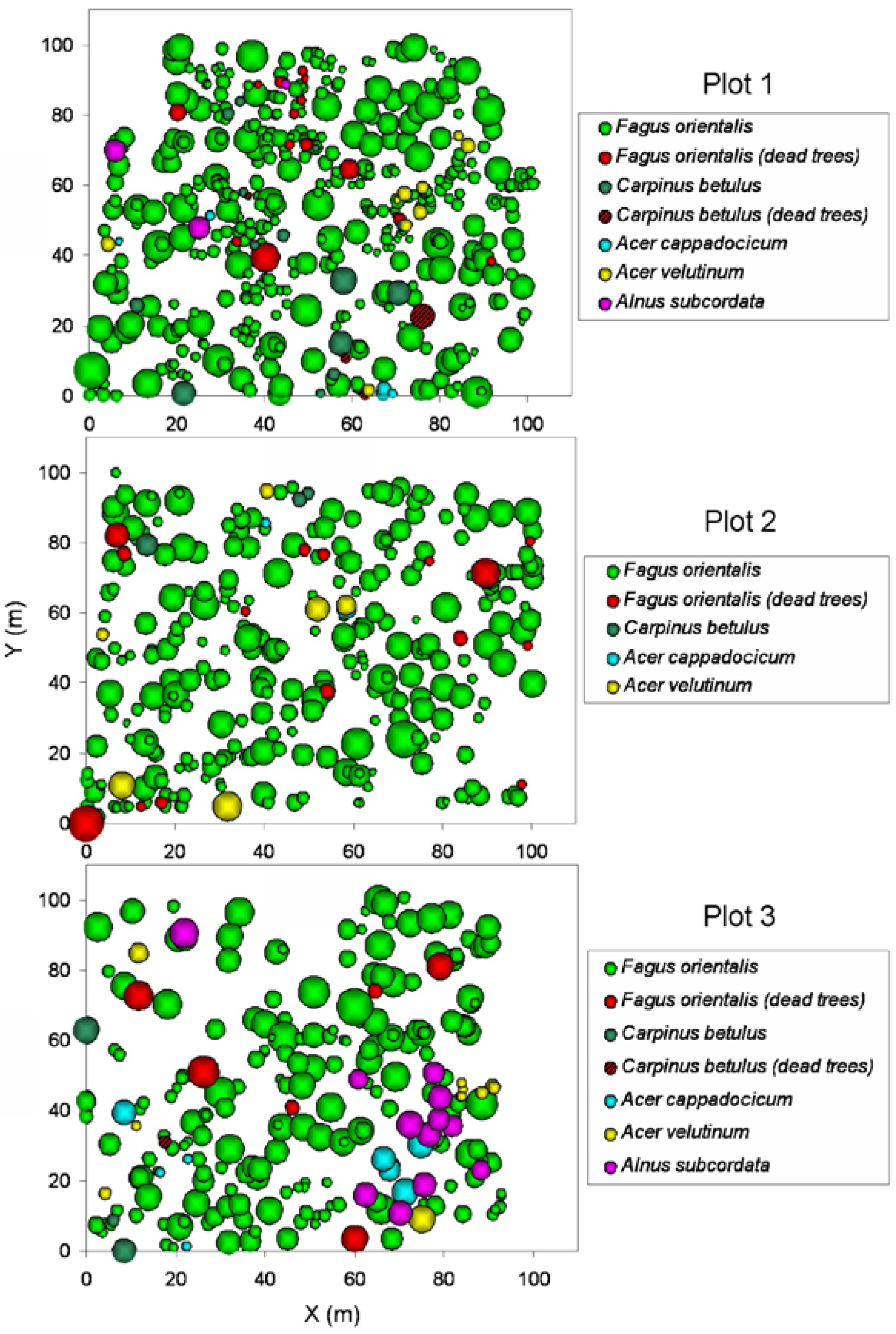
3.3. Spatial Analysis of Dead Trees

We detected significant spatial interactions (attraction) between living and dead beech trees at short to medium spatial scales (1–20 m) only in the plot 1, where patches of dead trees were evident (Figure 3 and Figure 4). In plots 2 and 3, we observed random spatial interactions and a non-significant trend towards repulsion (from 2 to 10 m) between living and dead beech trees. Only in plot 1 did living beech trees present significant spatial aggregation, but this was found only at 2-m scales.
Figure 3. Spatial pattern of trees in the studied plots from Shafaroud Region, northern Iran. Symbol size is proportional (about 1:10) to tree DBH.
Forests 04 00751 g003
Figure 4. Point pattern analyses of living and dead beech (F. orientalis) trees and other tree species (A. cappadocicum, A. velutinum, A. subcordata and C. betulus) in the three study plots. The figures show the observed bivariate pair-correlation function [g12(t)] as a function of distance, the 95% envelopes (dashed lines), and the expected g12(t) values based on the null model. Red points indicate significant positive interactions between dead and living beech trees. The goodness-of-fit test (GoF) of each analysis and its related probability level (P) are also displayed.
Forests 04 00751 g004

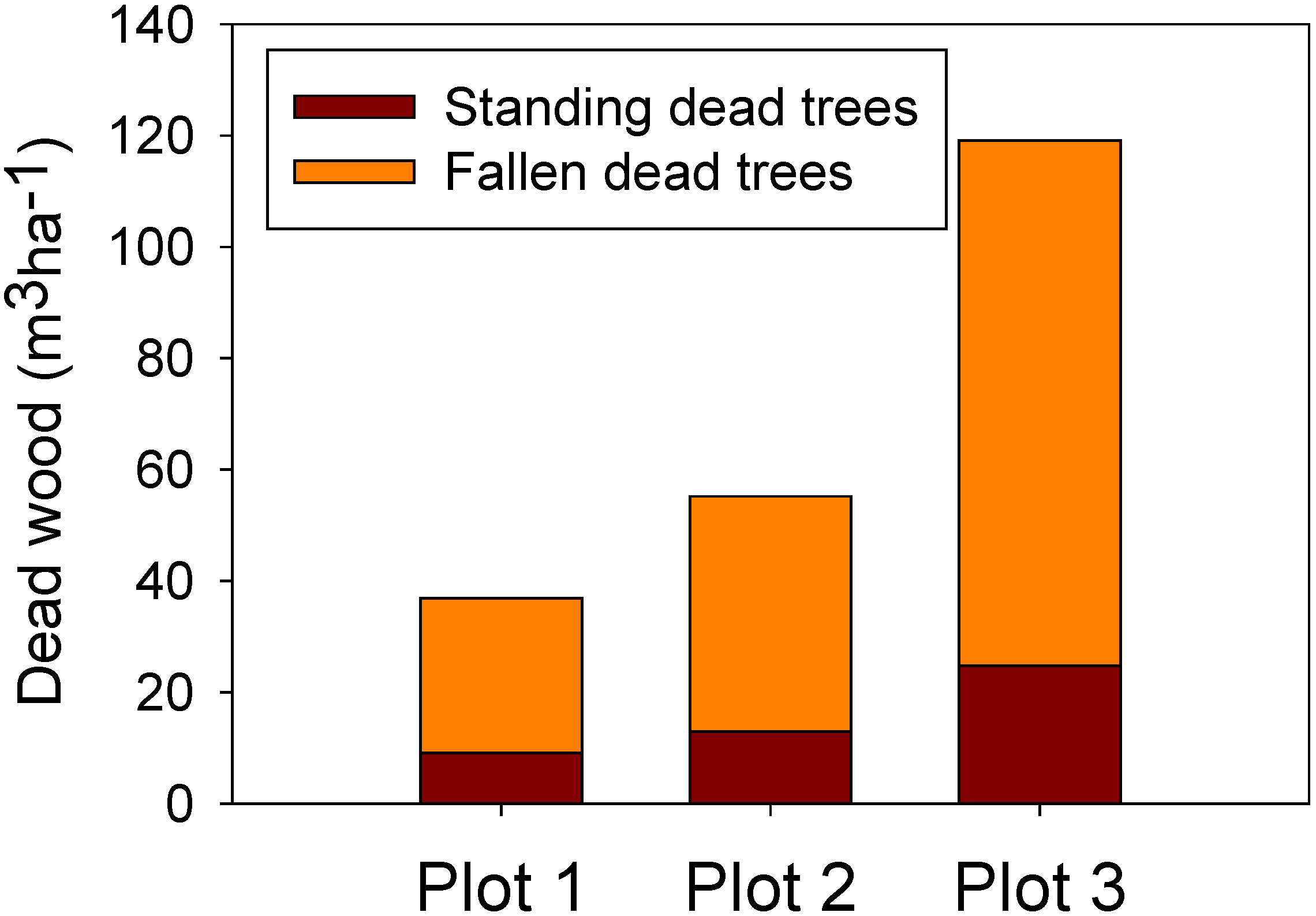
3.4. Volume of Dead Wood

The volume of standing dead trees in plots 1, 2, and 3 were 9, 13, and 25 m3 ha−1, respectively. Therefore, standing dead trees formed approximately 2%, 3%, and 6% of the total inventory in plots 1, 2, and 3, respectively. The volume of fallen dead trees ranged between 27.82 and 94.4 m3 ha−1, most of this in the plot 3 (21% of total inventory). The amount of total dead-wood volume was 7.5% in plot 1, 11.4% in plot 2, and 29% in plot 3. Overall, dead wood (standing and fallen trees) increased as stand density decreased (i.e., from plot 1 to plot 3; Table 3, Figure 5), ranging from 6% to 12%. More than 70% of fallen dead trees were classified within rot class III and IV in plot 1 and plot 2, while 55% of the fallen dead trees were classified within rot class III and IV in plot 3 (Table 4). A large number of the dead trees found in plot 1 appear to have died from competition (see also Figure 3).
Figure 5. Dead-wood volume for standing and fallen dead trees within the study plots.
Forests 04 00751 g005
Table 3. Wood volume recorded in the three study plots.
PlotLiving trees wood volume (m3 ha−1)Standing dead wood volume (m3 ha−1)Fallen dead wood volume (m3 ha−1)Dead wood volume to alive wood volume ratio (%)
1490.69.127.87.5
2486.012.942.311.4
3417.024.794.429.0
Table 4. Percentage of fallen trees within the different rot classes. Rot class I indicates recently fallen dead wood; rot class II indicates 25% decay; rot class III indicates 25%–50% decay; rot class IV indicates more than 50% decay.
Rot class (%)
IIIIIIIV
Plot 120103040
Plot 2008317
Plot 34412332

4. Discussion

Understanding the spatial distribution and volume of dead wood is especially important if the management goal is to mimic the dynamics of natural forest ecosystems [2,10]. Nevertheless, investigating these dynamics is difficult because temperate hardwood forest succession can span centuries, making data collection unrealistic [15]. Both the spatial pattern and amount of dead wood changed among our study plots, suggesting the presence of contrasting stand-development stages [21]. Many spatial statistical methods have been developed to quantify and model forest-stand dynamics, such as investigating tree mortality over succession by comparing the spatial patterns of dominant tree species in subsequent stages of a chronosequence [30,31,32]. Comparing the spatial patterns of dead trees in contrasting developmental stages provides a simple evaluation of the random-mortality hypothesis [33], which states that if mortality is a random event and every tree within the stand has an equal probability of death, there should be no significant spatial interaction between living and dead trees. By contrast, a positive aggregation between living and dead trees would indicate that tree-to-tree competition contributes to selective tree mortality within the stand [34].
In the present study, we took this approach to detect the importance of competition (spatially aggregated) and random tree-mortality patterns for a chronosequence of Caspian beech forests, including the characterization of the point patterns of dead trees, in addition to quantifications of total dead-wood volume. Typically, the locations of living and dead trees are analyzed for spatial pattern [30]; usually, such individuals are represented by point locations or coordinates derived through field stem mapping. As such, identification or detection of significant point patterns depends on the sampling-area size (as a scale subject). In our study, we used a plot surface area of one hectare, considered adequate to reveal the scale, extent, and dynamics of dead-tree patterns and allow the testing of potential hypotheses related to Caspian beech stand dynamics [21]. However, it should be noted that a higher number of mapped living and dead trees, within a vaster sampling area, would render more robust support for our conclusion [11]. Our results do suggest that a more extensive sampling area (plot surface) or a more intensive field survey focused on dead wood should be considered in further studies on spatial structure of dead trees in Caspian forests.
It is accepted that a transition from small-scale spatial aggregation to regular spatial pattern in subsequent stages of a chronosequence provides empirical evidence of intra-specific competition [31]. Our results support a spatial distribution shift from aggregation to randomness (even tending to regularity) for the dead trees analyzed in this study (Figure 4). This provides evidence suggesting that intra-specific competition governs the spatial distribution and population dynamics of F. orientalis-dominated forests [21]. Trees in high-density stands often suffer high mortality as a result of more intense neighborhood competition (see plot 1 in the Figure 3). As a result, the post-mortality spatial pattern of surviving trees shifts towards a more regularly spaced pattern (see plot 2 and 3 in Figure 3), providing evidence of density-dependent competition over the initial succession stages. This shift has been reported in uneven-aged temperate forests [35,36,37,38] and can be used to infer intra- and inter-specific interactions in mixed hardwood Caspian beech stands [21]. Moreover, if density-dependent competition is a decisive mechanism in the development of stand structure throughout succession, spatial regularity among older trees should increase over succession as individuals become larger and more effective competitors [34].
The non-random mortality observed in the plot 1 suggests that density-dependent mortality is a prevailing mechanism in F. orientalis-dominated forests. We found that dead trees were aggregated around living trees, suggesting that, in this stand, competition may be more important in the change of spatial pattern than stochastic or age-related mortality [35]. This significant spatial-aggregation pattern suggests an earlier growth stage in the plot 1, where light competition is typically high [15]. Hence, dead trees found in this plot seem to be related to overstory shading. This developmental stage was also characterized by an increasing proportion of small-diameter trees (mean tree diameters about 25 cm, total basal area about 39 m2 ha−1) and a decreasing amount of fallen dead wood. Plot 3, and to lesser extent plot 2, were characterized by increasing amounts of dead trees (particularly of large diameter and in a late stage of decay) following a regular spatial pattern.
On the other hand, spatial patterns in dead trees are consistent with previously documented gap-related regeneration dynamics in temperate beech forests [16,39]. Spatial analyses revealed a greater degree of small-scale dead-tree aggregation with greater tree density and smaller mean tree diameter [31]. This agrees with the expected pattern of gap-related regeneration—where recruits occupy gaps—likely created by the death of fallen old mature trees [40,41]. The succession pathway of the Caspian beech forests in northern Iran has been previously investigated [20,21,22,23,24]. Disturbances affecting Caspian hardwood forests appear to be critical for both regeneration and tree species diversity in these forest ecosystems [20]. Natural disturbances, such as windthrow, appear to have been necessary for recruitment or growth of many of the tree species within the canopy of these forests and, therefore, for their continued coexistence [16,42]. Furthermore, spatial variation in the frequency of disturbances and probably in their immediate effects would have determined the observed changes in stand structure and composition among our study plots.
Frequent low-intensity disturbances, rather than the hypothesized directional succession, are likely to have dominated the natural dynamics of Caspian beech forests for most of their history, including light and soil-nutrient changes as well as regeneration associated with these minor disturbances [40]. Mechanisms such as windthrow of dominant trees and further gap dynamics are known to drive stand structure and species composition [41]. However, competition for resources, primarily light, is also responsible for tree mortality [43], as revealed by the spatial association among living and dead trees (i.e., a non-random mortality spatial pattern). Relative light intensity on the forest floor of Caspian beech stands is commonly very dim due to F. orientalis canopy structure. Canopy gaps create patchy light and soil-nutrient availability, promoting tree regeneration (including beech and other species) and release [41]. Furthermore, as the mortality of overstory trees increases, additional gaps form, leading to the recruitment of smaller trees and to an increasingly aggregated individual spatial pattern (especially young cohorts). Thus, the spatial association among living and dead trees suggests a legacy effect from gap regeneration, currently resulting in tree-to-tree competition and self-thinning, which causes a spatial pattern shift from aggregation to overdispersion [32]. A lack of distinctive clustering of different cohorts should be expected as trees gain dominance through the mortality of other trees [43].
In terms of the amount of dead wood, we considered the volume of less than 30 m3 ha−1 to be small, 30–70 m3 ha−1 intermediate, and more than 70 m3 ha−1 large [6]. The total volume of dead wood, ranging from 37 to 119 m2 ha−1, varied greatly, even among different succession stages of the same forest. Indeed, in another study, such volumes estimated along a chronosequence of Caspian beech forest similar to those studied here also varied significantly among different succession stages [22]. In that study [22], the highest dead-wood volume was found in the late successional stages (51 m3 ha−1), while middle successional stages yielded about 26 m3 ha−1 and early successional stages registered 37 m3 ha−1 [22]. In general, the dead-wood volumes found in the present and others studies for Caspian beech forest were slightly below those reported in old-growth beech stands in Europe and North America [7,44]. Extensive studies covering most of the range of European beech (Fagus sylvatica L.) forests have indicated a mean dead-wood volume of about 130 m3 ha−1 [7], but between-site variation was also reportedly huge, ranging from almost nil to 550 m3 ha−1. Old-growth American beech (Fagus grandifolia Ehrh.) forests in Tennessee (USA) registered an average of 82–132 m3 ha−1 [44].
Dead-wood volume is significantly related to forest type, time span since the forest became unmanaged, and volume of living wood. Overall, dead-wood volumes tended to be higher in montane beech forests than in lowland or sub-montane forests, in stands with higher live tree volumes, and in long-time unmanaged forest than in recently protected [7]. For instance, studies performed in a near-to-natural European beech forest in Germany reported the amount of dead wood to be about 60 m3 ha−1, this exemplifying a relatively natural Central European beech forest (without any management since 1992 but under extensive management in the preceding 40 years) [45]. A study performed on European beech in northern Spain recorded a volume of standing and fallen dead wood of more than 30 m3 ha−1 after 80 years without significant human disturbance [46]. Although this volume of dead wood, which accumulated in less than one century, is relatively high, it was not of a large diameter (less than 40 cm diameter); old trees were uncommon, and no hollow trees were found [46]. Other studies conducted in near-to-natural beech forests reported dead-wood amounts ranging from 50 to 200 m3 ha−1 [7,47,48]; contrastingly, data from managed stands (e.g., in F. orientalis forests from Turkey) yielded a total dead-wood volume of about 23 m3 ha−1 [49,50].
At the same time, the density of standing dead trees declines in forest stands with increasing intensity of timber harvest and increasing ease of human access [51]. Furthermore, in addition to the average harvest interval, the abundance of standing dead trees in various stages of decay is also related to stand density and depth to the water table [19,52]. Finally, in relation to wood-decay stages, our results showed a high amount of wood within advanced decay classes. Recent models have indicated that wood-decay class transitions are related largely to wood-piece length and climatic regime, as transitions occurred more slowly for longer wood pieces located in regions with a low number of degree days (a climatic variable serving as a proxy for decomposition potential) [53]. Hardwood species transitioned into subsequent decay classes more rapidly than did softwoods [53]. In summary, dead wood appears to be a key component of natural forest, while managed forests show a significant decline in dead wood and therefore in most forest-dwelling organisms [5], specifically species dependent on dead-wood availability [6,7,8,9,10].

5. Conclusions

Mortality-driven changes in canopy composition are key in shaping Caspian beech forest structure and tree-species diversity. These changes seem to operate by different spatially structured processes across forest-succession stages, such as tree-to-tree competition and death by overstory shading at the stem-exclusion phase, and windthrow of dominant trees and further gap dynamics at the old-growth phase. Contrasting patterns of dead trees enhance spatial diversity and forest-structure complexity, where dead wood appears to be a major component of natural forests. The spatial distribution and volume of dead wood that result from natural tree mortality may serve as a management target in near-to-natural Caspian beech forest. On the basis of our results, conservation-oriented management strategies should account for increasing the amount of dead wood, particularly of large diameter and at a late stage of decay.

Conflicts of Interest

The authors declare no conflict of interest.

Acknowledgements

The authors would like to thank the Forest, Range and Watershed Organization of Iran for the financial support of the project. Jesús Julio Camarero acknowledges the support of ARAID. David Nesbitt looked over the English of this manuscript.

References

  1. Peterken, G.F. Natural Woodland: Ecology and Conservation in Northern Temperate Regions; Cambridge University Press: Cambridge, UK, 1996. [Google Scholar]
  2. Gossner, M.M.; Lachat, T.; Brunet, J.; Isacsson, G.; Bouget, C.; Brustel, H.; Brandl, R.; Weisser, W.W.; Müller, J. Current near-to-nature forest management effects on functional trait composition of saproxylic beetles in Beech Forests. Conserv. Biol. 2013, 27, 605–614. [Google Scholar] [CrossRef]
  3. Standovár, T.; Kenderes, K. A review on natural stand dynamics in beech woods of east central Europe. Appl. Ecol. Env. Res. 2003, 1, 19–46. [Google Scholar]
  4. Linares, J.C.; Carreira, J.A.; Ochoa, V. Human impacts drive forest structure and diversity. Insights from Mediterranean mountain forest dominated by Abies pinsapo. Eur. J. For. Res. 2011, 130, 533–542. [Google Scholar] [CrossRef]
  5. Kirby, K.J.; Reid, C.M.; Thomas, R.C.; Goldsmith, F.B. Preliminary estimates of fallen dead wood and standing dead trees in managed and unmanaged forests in Britain. J. Appl. Ecol. 2007, 35, 148–155. [Google Scholar]
  6. Lassauce, A.; Paillet, Y.; Jactel, H.; Bouget, C. Deadwood as a surrogate for forest biodiversity: Meta-Analysis of correlations between deadwood volume and species richness of saproxylic organisms. Ecol. Indic. 2011, 11, 1027–1039. [Google Scholar] [CrossRef]
  7. Christensen, M.; Hahn, K.P.; Mountford, E.; Odor, M. Dead wood in European beech (Fagus sylvatica) forest reserves. For. Ecol. Manag. 2005, 210, 267–282. [Google Scholar] [CrossRef]
  8. Stokland, J.N.; Siitonen, J. Biodiversity in Dead Wood; Cambridge University Press: Cambridge, UK, 2012. [Google Scholar]
  9. Heilmann-Clausen, J.; Christensen, M. Does size matter? On the importance of various dead wood fractions for fungal diversity in Danish beech forests. For. Ecol. Manag. 2004, 201, 105–117. [Google Scholar]
  10. Brunet, J.; Fritz, O.; Richnau, G. Biodiversity in European beech forests—A review with recommendations for sustainable forest management. Ecol. Bull. 2010, 53, 77–94. [Google Scholar]
  11. Diggle, P.J. Statistical Analysis of Point Patterns; Arnold: London, UK, 2003. [Google Scholar]
  12. Arevalo, J.R.; Fernandez-Palacios, J.M. Spatial patterns of trees and juveniles in a laurel forest of Tenerife, Canary Islands. Plant Ecol. 2003, 165, 1–10. [Google Scholar] [CrossRef]
  13. Tilman, D. Competition and biodiversity in spatially structured habitats. Ecology 1994, 75, 2–16. [Google Scholar] [CrossRef]
  14. Szwagrzyk, J.; Szewczyk, J. Tree mortality and effects of release from competition in an old-growth Fagus-Abies-Picea stand. J. Veg. Sci. 2001, 12, 621–626. [Google Scholar] [CrossRef]
  15. Oliver, C.D.; Larson, B.C. Forest Stand Dynamics; Wiley: New York, NY, USA, 1996. [Google Scholar]
  16. Lorimer, C.G.; White, A.S. Scale and frequency of natural disturbances in the Northeastern United States: Implications for early successional forest habitats and regional age distributions. For. Ecol. Manag. 2003, 185, 41–64. [Google Scholar] [CrossRef]
  17. Saniga, M.; Schutz, J.P. Relation of dead wood course within the development cycle of selected virgin forests in Slovakia. For. Sci. 2002, 48, 513–528. [Google Scholar]
  18. Mountford, E. Fallen and dead wood levels in the near-nature beech at La Tillaie Reserve, Fontainebleau, France. Oxf. For. Inst. For. 2002, 75, 203–208. [Google Scholar]
  19. Aakala, T.; Kuuluvainen, T.; Gauthier, S.; Grandpré, L. Standing dead trees and their decay-class dynamics in the north eastern boreal old-growth forests of Quebec. For. Ecol. Manag. 2008, 255, 410–420. [Google Scholar] [CrossRef]
  20. Parhizkar, P.; Sagheb-Talebi, K.; Mataji, A.; Namiranian, M. Influence of gap size and development stages on the silvicultural characteristics of oriental beech (Fagus orientalis Lipsky) regeneration. Caspian J. Env. Sci. 2011, 9, 55–65. [Google Scholar]
  21. Akhavan, R.; Sagheb-Talebi, Kh.; Zenner, E.K.; Safavimanesh, F. Spatial patterns in different forest development stages of an intact old-growth Oriental beech forest in the Caspian region of Iran. Eur. J. For. Res. 2012, 131, 1355–1366. [Google Scholar] [CrossRef]
  22. Sefidi, K.; Marvie-Mohadjer, M.R. Characteristics of coarse woody debris in successional stages of natural beech (Fagus orientalis) forests of Northern Iran. J. For. Sci. 2010, 56, 7–17. [Google Scholar]
  23. Zolfaghari, E.; Marvi Mohajer, M.R.; Namiranian, M. Impact of dead trees on natural regeneration in forest stands (Chelir District, Kheiroudkenar, Now-shahr). Iran. J. For. Poplar Res. 2007, 15, 234–240. [Google Scholar]
  24. Habashi, H. Study of Ecological and Silvicultural Importance of Dead Trees in Nour Forests. Master Thesis, University of Tarbiat Modarres, Tehran, Iran, 1998. [Google Scholar]
  25. Muller-Using, S.; Bartsch, N. Dynamics of Woody Debris in A Beech (Fagus sylvatica L.) Forest in Centeral Germany. In Proceeding of the 7th International Beech Symposium, Tehran, Iran, 10–20 May 2004; pp. 83–89.
  26. Nordén, B.; Ryberg, M.; Götmark, F.; Olausson, B. Relative importance of coarse and fine woody debris for the diversity of wood-inhabiting fungi in temperate broadleaf forests. Biol. Conserv. 2004, 117, 1–10. [Google Scholar] [CrossRef]
  27. Goreaud, F.; Pèlissier, R. Avoiding misinterpretation of biotic interactions with the intertype K12-function: Population independence vs. random labelling hypotheses. J. Veg. Sci. 2004, 14, 681–692. [Google Scholar]
  28. Stoyan, D.; Stoyan, H. Fractals, Random Shapes and Point Fields: Methods of Geometrical Statistics; Wiley: Chichester, UK, 1994. [Google Scholar]
  29. Wiegand, T.; Moloney, K.A. Ring, circles, and null-models for point pattern analysis in ecology. Oikos 2004, 104, 209–229. [Google Scholar] [CrossRef]
  30. He, F.; Legendre, P.; LaFrankie, J.V. Distribution patterns of tree species in a Malaysian tropical rain forest. J. Veg. Sci. 1997, 8, 105–114. [Google Scholar] [CrossRef]
  31. Gray, L.; He, F. Spatial point-pattern analysis for detecting density-dependent competition in a boreal chronosequence of Alberta. For. Ecol. Manag. 2009, 259, 98–106. [Google Scholar] [CrossRef]
  32. He, F.; Duncan, R.P. Density-dependent effects on tree survival in old-growth Douglas fir forest. J. Ecol. 2000, 88, 676–688. [Google Scholar] [CrossRef]
  33. Little, L.R. Investigating competitive interactions from spatial patterns of tree in multi-space boreal forests: The random mortality hypothesis revisited. Can. J. Bot. 2002, 80, 93–100. [Google Scholar] [CrossRef]
  34. Getzin, S.; Dean, C.; He, F.; Trofymow, J.A.; Wiegand, K.; Wiegand, T. Spatial patterns and competition of tree species in a Douglas-fir chronosequence on Vancouver Island. Ecography 2006, 29, 671–682. [Google Scholar] [CrossRef]
  35. Duncan, R.P. Competition and the coexistence of species in a mixed podocarp stand. J. Ecol. 1991, 79, 1073–1084. [Google Scholar] [CrossRef]
  36. Rozas, V.; Zas, R.; Solla, A. Spatial structure of deciduous forest stands with contrasting human influence in northwest Spain. Eur. J. For. Res. 2009, 128, 273–285. [Google Scholar] [CrossRef]
  37. Veblen, T.T.; Ashton, D.H.; Schlegel, F.M. Tree regeneration strategies in a lowland Nothofagus-dominated forest in southcentral Chile. J. Biogeo. 1979, 6, 329–340. [Google Scholar] [CrossRef]
  38. Salas, C.; LeMay, V.; Nunez, P.; Pacheco, P.; Espinosa, A. Spatial patterns in an old-growth Nothofagus oblique forest in south central Chile. For. Ecol. Manag. 2006, 231, 38–46. [Google Scholar] [CrossRef]
  39. Peters, R.; Poulson, T.L. Stem growth and canopy dynamics in a world-wide range of Fagus forests. J. Veg. Sci. 1994, 5, 421–432. [Google Scholar] [CrossRef]
  40. Canham, C.D. Growth and canopy architecture of shade tolerant trees. Response to canopy gaps. Ecology 1988, 69, 786–795. [Google Scholar] [CrossRef]
  41. Canham, C.D. Suppression and release during canopy recruitment in Fagus grandifolia. Bull. Torrey Bot. Club 1990, 117, 1–7. [Google Scholar] [CrossRef]
  42. Attiwill, P.M. The disturbance of forest ecosystems: The ecological basis for conservation management. For. Ecol. Manage. 1994, 63, 247–300. [Google Scholar] [CrossRef]
  43. Olano, J.M.; Laskurain, N.A.; Escudero, A.; de La Cruz, M. Why and where do adult trees die in a young secondary temperate forest? The role of neighbourhood. Ann. For. Sci. 2009, 66, 105–112. [Google Scholar] [CrossRef] [Green Version]
  44. Harmon, M.E.; Franklin, J.F.; Swanson, F.J.; Sollins, P.; Gregory, S.V.; Lattin, J.D.; Anderson, N.H.; Cline, S.P.; Aumen, N.G.; Sedell, J.R.; et al. Ecology of coarse woody debris in temperate ecosystems. Adv. Ecol. Res. 1986, 15, 133–276. [Google Scholar] [CrossRef]
  45. Beneke, C.; Manning, D. Coarse Woody Debris (CWD) in the Weberstedter Holz, A near Natural Beech Forest in Central Germany. Presented at Part of Deliverable 20 of the Nat-Man project (Nature based Management of Beech in Europe); Albert-Ludwigs University: Thuringia, Germany, 2003; p. 18. Available online: http://sl.life.ku.dk/English/research/forest_and_ecology/silviculture/natman/natural_beech_forests/~/media/Sl/Forskning_Research/Skov_oekologi/natman/reports/deliverable_20_part_beneke_christian.ashx (accessed on 6 May 2013).
  46. Castro-Gil, A. Evolution and structure of Artikutza, an 80-year old beech forest in Navarra (northern Spain). Munibe (Cienc. Nat. Nat. Zientziak) 2009, 57, 257–281. [Google Scholar]
  47. Motta, R.; Berretti, R.; Lingua, E.; Piussi, P. Coarse woody debris, forest structure and regeneration in the Valbona Forest Reserve, Paneveggio. Ital. Alps. For. Ecol. Manag. 2006, 235, 155–163. [Google Scholar] [CrossRef]
  48. Piovesan, G.; di Filippo, A.; Alessandrini, A.; Biondi, F.; Schirone, B. Structure, dynamics and dendroecology of an old-growth Fagus forest in the Apennines. J. Veg. Sci. 2005, 16, 13–28. [Google Scholar]
  49. Atici, E.; Colak, A.H.; Rotherhm, I.D. Coarse dead wood volume of managed oriental beech (Fagus orientalis Lipsky) stands in Turkey. For. Syst. 2008, 17, 216–227. [Google Scholar]
  50. Colak, A.; Tokcan, M.; Rotherham, I.; Atici, E. The amount of coarse dead wood and associated decay rates in forest reserves and managed forests, northwest Turkey. For. Syst. 2009, 18, 350–359. [Google Scholar]
  51. Wisdom, M.J.; Bate, L.J. Snag density varies with intensity of timber harvest and human access. For. Ecol. Manag. 2008, 255, 2085–2093. [Google Scholar] [CrossRef]
  52. Russell, M.B.; Kenefic, L.S.; Weiskittel, A.R.; Puhlick, J.J.; Brissette, J.C. Assessing and modeling standing deadwood attributes under alternative silvicultural regimes in the Acadian Forest region of Maine, USA. Can. J. For. Res. 2012, 42, 1873–1883. [Google Scholar] [CrossRef]
  53. Russell, M.B.; Woodall, C.W.; Fraver, S.; D’Amato, A.W. Estimates of downed woody debris decay class transitions for forests across the eastern United States. Ecol. Model. 2013, 251, 22–31. [Google Scholar] [CrossRef]

