Article

Are the Economically Optimal Harvesting Strategies of Uneven-Aged Pinus nigra Stands Always Sustainable and Stabilizing?

by
Ignacio López-Torres
1,*,
Sigfredo Ortuño-Pérez
1,
Fernando García-Robredo
1 and
Carmen Fullana-Belda
2
1
Universidad Politécnica de Madrid, ETSI de Montes, Ciudad Universitaria, 28040 Madrid, Spain
2
Universidad Pontificia de Comillas, Alberto Aguilera, 23, 28015 Madrid, Spain
*
Author to whom correspondence should be addressed.
Forests 2013, 4(4), 830-848; https://doi.org/10.3390/f4040830
Submission received: 26 July 2013 / Revised: 22 September 2013 / Accepted: 30 September 2013 / Published: 18 October 2013

Abstract

:
Traditional uneven-aged forest management seeks a balance between equilibrium stand structure and economic profitability, which often leads to harvesting strategies concentrated in the larger diameter classes. The sustainability (i.e., population persistence over time) and influence of such economically optimal strategies on the equilibrium position of a stand (given by the stable diameter distribution) have not been sufficiently investigated in prior forest literature. This article therefore proposes a discrete optimal control model to analyze the sustainability and stability of the economically optimal harvesting strategies of uneven-aged Pinus nigra stands. For this model, we rely on an objective function that integrates financial data of harvesting operations with a projection matrix model that can describe the population dynamics. The model solution reveals the optimal management schedules for a wide variety of scenarios. To measure the distance between the stable diameter distribution and the economically optimal harvesting strategy distribution, the model uses Keyfitz’s delta, which returns high values for all the scenarios and, thus, suggests that those economically optimal harvesting strategies have an unstabilizing influence on the equilibrium positions. Moreover, the economically optimal harvesting strategies were unsustainable for all the scenarios.

1. Introduction

The goal of traditional uneven-aged forest management is a balance between equilibrium stand structure and economic profitability. In pursuing this balance, many harvesting strategies concentrateon the larger diameter classes. The sustainability (i.e., population persistence over time) and influence of such economically optimal strategies on the equilibrium position of a stand (given by the stable diameter distribution) have not been sufficiently investigated in prior forest literature. Using uneven-aged Pinus nigra stands as an example, we propose a discrete optimal control model that can assess whether the economically optimal harvesting strategies are sustainable or stabilizing. For this model, we rely on an objective function that integrates the financial data of harvesting operations with a matrix model that can describe the population dynamics.
Matrix models commonly serve to analyze the evolution, management and harvesting of tree populations [1,2,3,4]. Population growth rate in such models is the dominant eigenvalue, λ0, of the transition matrix, A. According to asymptotic analysis (i.e., long-term behavior), we know that independent of the initial conditions, when λ0 >1, the total number of stems/ha of the tree population increases exponentially over time (without harvests), whereas when λ0 < 1, the population decays until extinction, and when λ0 = 1, the result is a stable distribution proportional to the right eigenvector, W0, of the transition matrix that corresponds to λ0. Gotelli [5] refers to the special case of the stable distribution when λ0 = 1 as the “stationary distribution”; we consider a similar case in reference to the stable diameter distribution of the stand W0.
This concept of stability relates closely to the concept of perturbation: A system is stable if it always returns to an equilibrium position following small perturbations (otherwise, the system is unstable). The stable distributions are closely dependent on recruitment, removal and stem migration throughout the diameter at breast height (dbh)-classes over time [6]. In fact, given the transition probabilities between diameter classes, for each pair (R, G), where G is the stand basal area and R is the global amount of recruitment, the stable diameter distributions of managed uneven-aged Fagus sylvatica L. and Pinus nigra Arn. stands were calculated in [7,8,9] using a matrix model of stand diameter classes evolution. Those stable diameter distributions are associated with the “sustainable/stable” harvesting strategy [7,8], aimed at reaching in each harvest the proportions of stems/ha in each class corresponding to the stable diameter distribution of the stand, yielding the following “sustainable/stable” harvest rate:
Forests 04 00830 i001
for all the diameter classes and time steps. This rate corresponds to the case in which the right eigenvector associated with the dominant eigenvalue λ = 1 of the transition matrix with harvests is W0.
Therefore, in the present study, we combine that matrix model to describe the population dynamics with an economic model (objective function) that summarizes the net present value (NPV) of all the management operations in a 70-year harvest cycle, which creates a discrete optimal control problem.
Optimal control theory enables the solution of a wide variety of dynamic problems, for which the evolution of the dynamic system (discrete or continuous) can be partially controlled by the agent’s decision. In every moment, t, the system can be described by a set of state variables, xk(t) (e.g., stems/ha in diameter class k at year t), so the planner chooses a specific set of control variables, hk(t) (e.g., the harvest rate in diameter class k at year t). Different values for the control variables imply different paths in the phase space for the dynamic system, and the planner or manager must determine the control values that maximize the selected objective, according to the constraints of the problem.
Many authors have considered optimal control theory to model forest stands (e.g., continuous case, [10,11]; discrete case, [12,13,14]).
Thus, the main purpose of this study is to determine economically optimal harvesting strategies of uneven-aged Pinus nigra stands in the Spanish Iberian System and to analyze their sustainability and eventual destabilization (i.e., with the stable diameter distribution W0 set as the initial condition, to discern if the introduction of an NPV maximizing management strategy leads to distributions that move away from that equilibrium over time). Furthermore, we investigate the effects of diameter growth, stand density and recruitment on those strategies, considering a wide variety of typical management scenarios in the study area, obtained by combining three levels of diameter growth (Qualities IIII), three levels of stand basal area, G = 22, 24 and 26 m2/ha, and three levels of global recruitment, R = 200, 520 and 840 stems/ha. Finally, an economic comparison has been performed between the economically optimal and the “sustainable/stable” harvesting strategies.
In the following sections, we describe the model and the estimates of the corresponding parameters. The general calculations, including regressions, were run using Maple version 16 [15], and the solutions to the optimization problems were derived from Solver Premium Platform version 7.1 [16] running under Excel 2010.

2. Material and Methods

2.1. Population Dynamics

The model for recruitment, harvesting and stem migration throughout the dbh classes over time is based on the model proposed by López et al. [7,8] for Fagus sylvatica L. and by López et al. [9] for Pinus nigra Arn. stands. In this case, the stands of the study area are located in the Spanish Iberian System, a mountain range extending about 400 km along the north-eastern edge of the central plateau, concentrating 60% of the area occupied by Pinus nigra in Spain [17]. The management of Pinus nigra stands in this area is currently based on the growth and yield tables for Pinus nigra Arn. in the Spanish Iberian System [18]. The data in these tables are classified according to growth level into five site qualities, of which only the first three have been selected as our data source. These three qualities (I, faster; II, medium; and III, slower diameter growth) were defined by the dominant heights reached at the reference age of 60 years (20, 17 and 14 m, respectively).
The starting assumptions were as follows: (a) the forest is in a steady state; (b) the average diameter growth curves for Qualities IIII are defined by the Bertalanffy-Richards model; (c) within each diameter class, the probability distribution for the diameter of the trees is uniform (rectangular); and (d) harvesting operations occur at the beginning of every projection interval.
Harvesting operations in this study area generally took place every 10 years, so we adopted this period as the range of the projection intervals in the model. Considering this time period and the diameter growth functions corresponding to Qualities IIII, trees were grouped into n diameter classes of equal width w = 6 cm: (0,6), (6,12), (12,18), ..., (30,36),…, with the last class being (48,→) (more than 48 cm) for Quality I, (42,→) (more than 42 cm) for Quality II and (36,→) (more than 36 cm) for Quality III. Therefore, an individual tree in class k can remain in class k or progress to class k + 1 during the projection interval (t, t + 10). The number of trees in each class changed in each projection interval, because some were harvested, some remained in the same diameter class and others grew past the boundary to the next diameter class. In such conditions, pk refers to the probability that an individual tree in class k at time t will appear in class k + 1 at time t + 10. The term, rk, or the recruitment coefficient, is the number of offspring (stems/ha) living at time t + 10 produced in the interval (t, t + 10) by an average tree in class k at time t (Similar to many standard size classified matrix models, we did not consider the smallest diameter class fertile.). The variable, hk(t), defines the proportion of harvested trees in class k at year t, natural mortalities included. Finally, xk(t) and xk(t + 10) describe the stem densities in class k at the initial and final projection times. By analyzing the dynamics of the projections, we find that the model is described accurately by the matrix model:
X(t + 10) = A(IH(t)) X(t),
Where:
Forests 04 00830 i002
I is the identity matrix, H(t) = diag( h1(t), h2(t) , …, hn(t) ) is a diagonal matrix with the harvest rates hk(t) and X(t) and X(t + 10) are column vectors indicating the stem densities at the initial and final times of projection, respectively.

2.2. Optimization Model

Since the main objective for the stands in the study area is the production of timber, we use, as the objective function of the optimization problem, the net present value of all the management operations over a time horizon of T = 70 years, discounted to the beginning of the period, and from the landowner’s perspective. The combination of this objective function with the population dynamics model produces a discrete optimal control problem, from which we have to determine control variables hk(t) that globally maximize the function:
Forests 04 00830 i003
where xk(t), or the state variables, represent the number of stems/ha in class k at year t, hk(t), or the control variables, define the harvest rate in class k at year t, vk(t) is the stumpage price that corresponds to class k at year t (euro/stem), i is the discount rate and T is the planning horizon in years (where k = 1, 2, … , n and t = 0, 10, 20, … , T–10 years). The first summation represents the income derived from the sale of timber, and the last is the final stocking value. It is well known that the NPV is a justifiable management objective for a single economic goal [19].
As commented on in the Introduction, the initial conditions must represent the stable diameter distributions of the stand or X(0) = W0.
We also introduce the following constraints:
mkhk(t) ≤ 1 for k = 1, 2, … , n and t = 0, 10, 20, 30, … , T − 10,
where mk is the natural mortality in class k.
By applying the “sustainable/stable” harvesting strategy to each scenario and setting X(0) = W0 (stable diameter distribution) as the initial condition, the basal area of the stand continuously oscillates between the Gmin (after harvesting) and Gmax (before harvesting) values, and the stable diameter distribution is reached at each time step. Therefore, in order to compare the economically optimal and the “sustainable/stable” harvesting strategies, it is essential to assume an additional constraint to maintain the stand basal area throughout the harvest cycle within the range GminGmax (where Gmax = 22 for the G = 22 m2/ha scenario, Gmax = 24 for G = 24 m2/ha, Gmax = 26 for G = 26 m2/ha and Gmin is the minimum basal area reached for each scenario under the “sustainable/stable” harvesting strategy) during the optimization process.

2.3. Input Estimation

2.3.1. Transition Probabilities

We calculated the transition probabilities by applying the method introduced by López et al. [9] considering that, given the basal area constraints and the low basal area scenarios of this study, stand density has small influence on diameter growth. Thus, the diameter growths were defined by the Bertalanffy-Richards function:
D = f(t) = a(1 − ebt)c
adjusted using regressiona nalysis to data points (t, D(t)) in Gómez-Loranca’s tables [18]. The main characteristics of these growth models for Qualities I–III are shown in Figure 1.
Using these diameter growth models, the transition probabilities from class i to class (i + 1), or from interval (6(i − 1), 6i) to interval (6i, 6(i + 1)), are given by:
Forests 04 00830 i004
where f-1, the inverse function of f in (1), is defined by:
Forests 04 00830 i005
(where t is age in years and D is dbh in cm).
Figure 1. Diameter growth models: Quality I, D = 51.68 (1 − e−0.015259·t)1.255111; Quality II, D = 46.645633 (1 − e−0.014318·t)1.337062; and Quality III, D = 40.644134 (1 − e−0.013838)1.456382 (dbh, D, in cm and time t in years). The coefficient of determination was always greater than 0.999.
Forests 04 00830 g001
The above mentioned transition probability formula is a direct application of the one introduced by López et al. [7,8] for a Bertalanffy-Richards model. We provide the calculations for Qualities IIII in Table 1.
Table 1. Transition probabilities between diameter classes for each quality.
Quality IQuality IIQuality III
(0,6) → (6,12)p1 = 0.7697p1 = 0.5951p1 = 0.4564
(6,12) → (12,18)p2 = 0.8602p2 = 0.6824p2 = 0.5326
(12,18) → (18,24)p3 = 0.7913p3 = 0.6200p3 = 0.4697
(18,24) → (24,30)p4 = 0.6828p4 = 0.5190p4 = 0.3692
(24,30) → (30,36)p5 = 0.5533p5 = 0.3971p5 = 0.2475
(30,36) → (36,42)p6 = 0.4106p6 = 0.2618p6 = 0.1119
(36,42) → (42,48)p7 = 0.2587p7 = 0.1171-
(42,48) → (48,→)p8 = 0.1000--
According to the model assumptions and the methodology used, we had to consider that the same transition probability, pk, applies to all the individuals in the same class k, where there might exist individuals under very different conditions (that is, the transition probability pk is a global property shared by all the individuals in the same class k, independently of their local conditions). We consider that the stratification into three quality classes must result in low variability around the mean pk values.

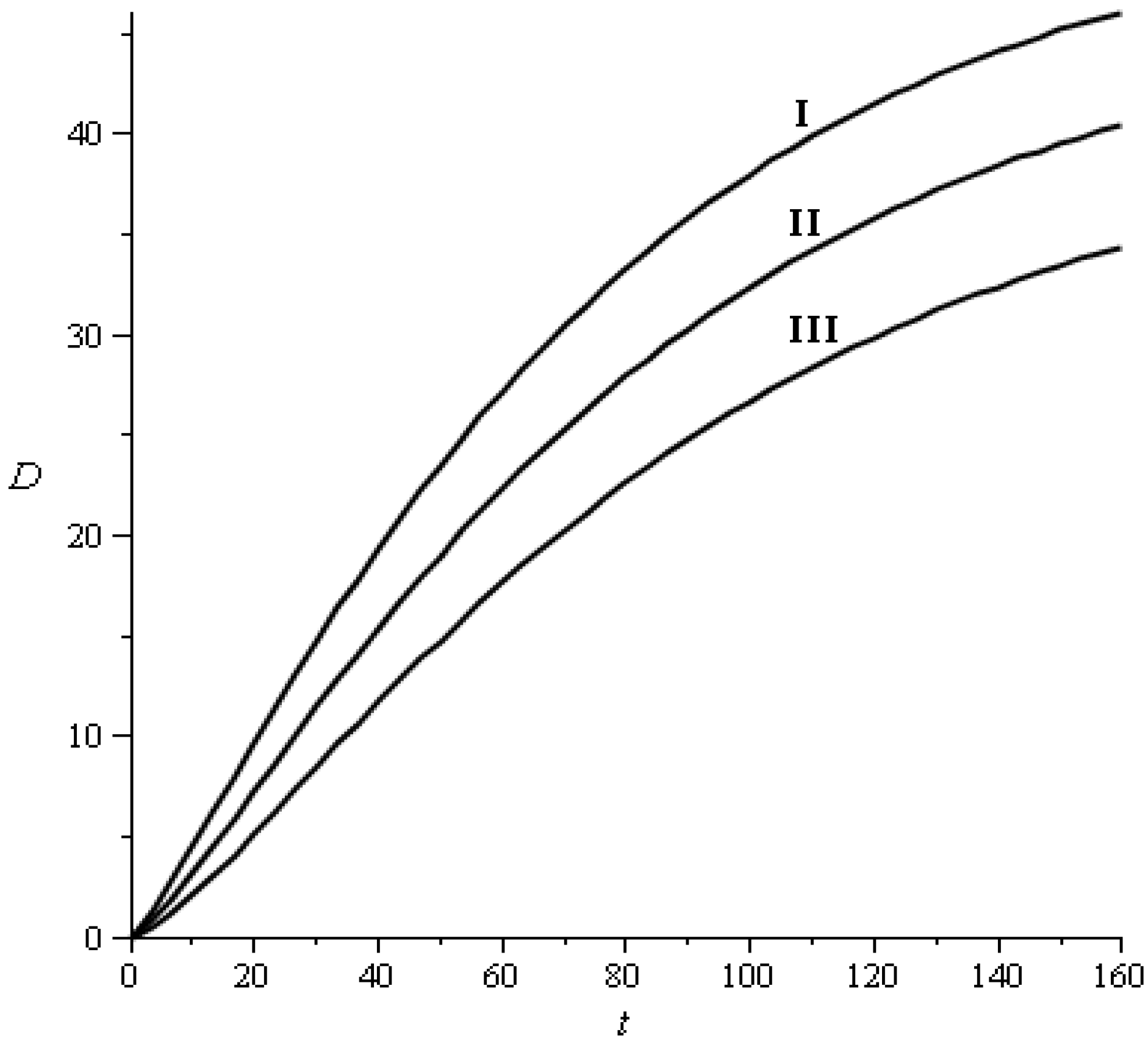
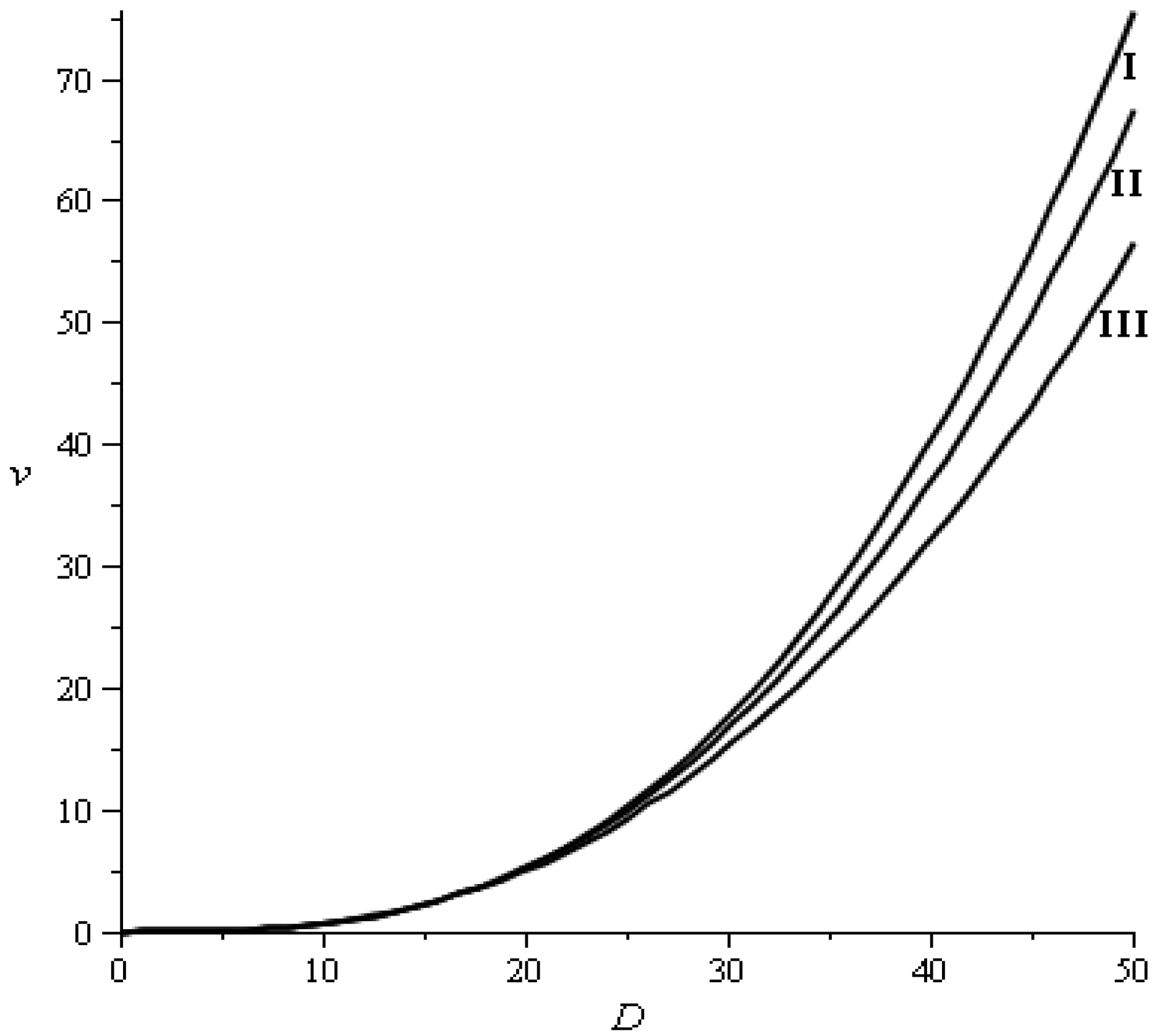
2.3.2. Recruitment and Basal Area

Although Pinus nigra regenerates well under its own canopy [20,21] and recruitment may be very abundant even at high densities (more than 1,875 stems/ha during a regeneration in Pinus nigra stands where G = 51.96 m2/ha, as described in [22]), there is a critical basal area for sufficient light transmittance for regeneration, that is, approximately 20–30 m2/ha [23,24]. Therefore, we have considered in the calculations three levels of stand basal area in that range, G = 22, 24 and 26 m2/ha. With these basal area values, we have assumed the same three levels of recruitment of our previous studies, R = 200 (scarce recruitment), 520 (normal recruitment) and 840 (abundant recruitment) stems/ha. For these cases, similar to other matrix models for tree species [25], we attributed the global amount of recruitment R entirely to the last diameter class (r2 = r3 = … = rn-1 = 0; rn = Forests 04 00830 i006), which had no influence on the stable diameter distribution of the stand, which is established by transition probabilities, the global amount of recruitment and stand basal area [7].

2.3.3. Natural Mortalities

We estimated natural mortalities using previous studies. Specifically, Misir et al. [26] developed a logistic mortality model for Pinus nigra subsp. pallasiana in Turkey, and from the observed data, they estimated an overall annual mortality rate of 1.41%, equivalent to a 13.24% mortality rate in a 10-year period. Trasobares and Pukkala [27] studied Pinus nigra Arn. in north-eastern Spain and suggested natural mortality rates (including minimal intermediate thinning) of 2% for the D > 30 cm diameter classes.
We thus assumed the following 10-year individual tree constant mortality rates for each diameter class: m1 = 0.20, m2 = 0.14, m3 = 0.08, m4 = 0.05, m5 = 0.03 and m6 = m7 = … = mn = 0.02.

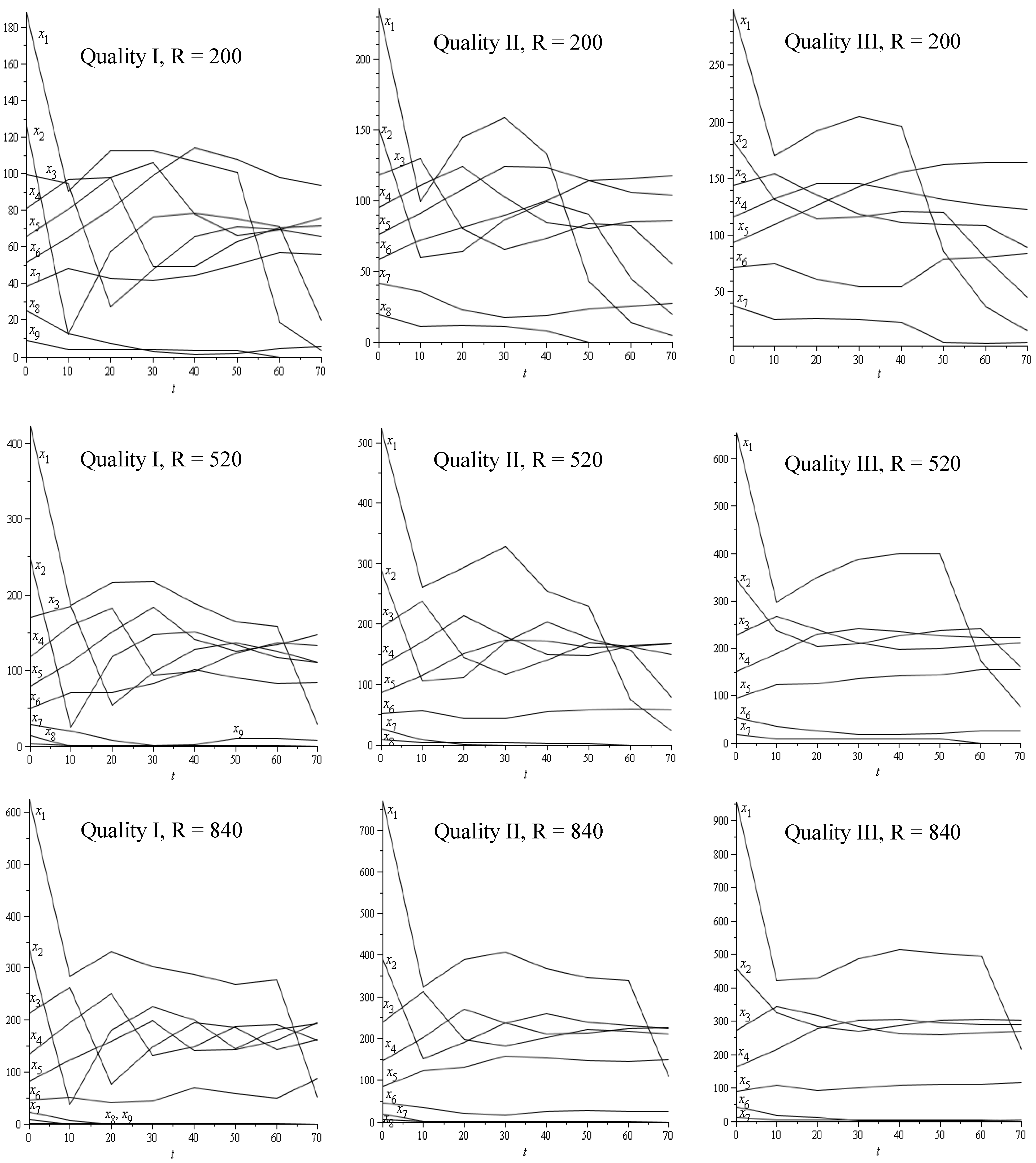
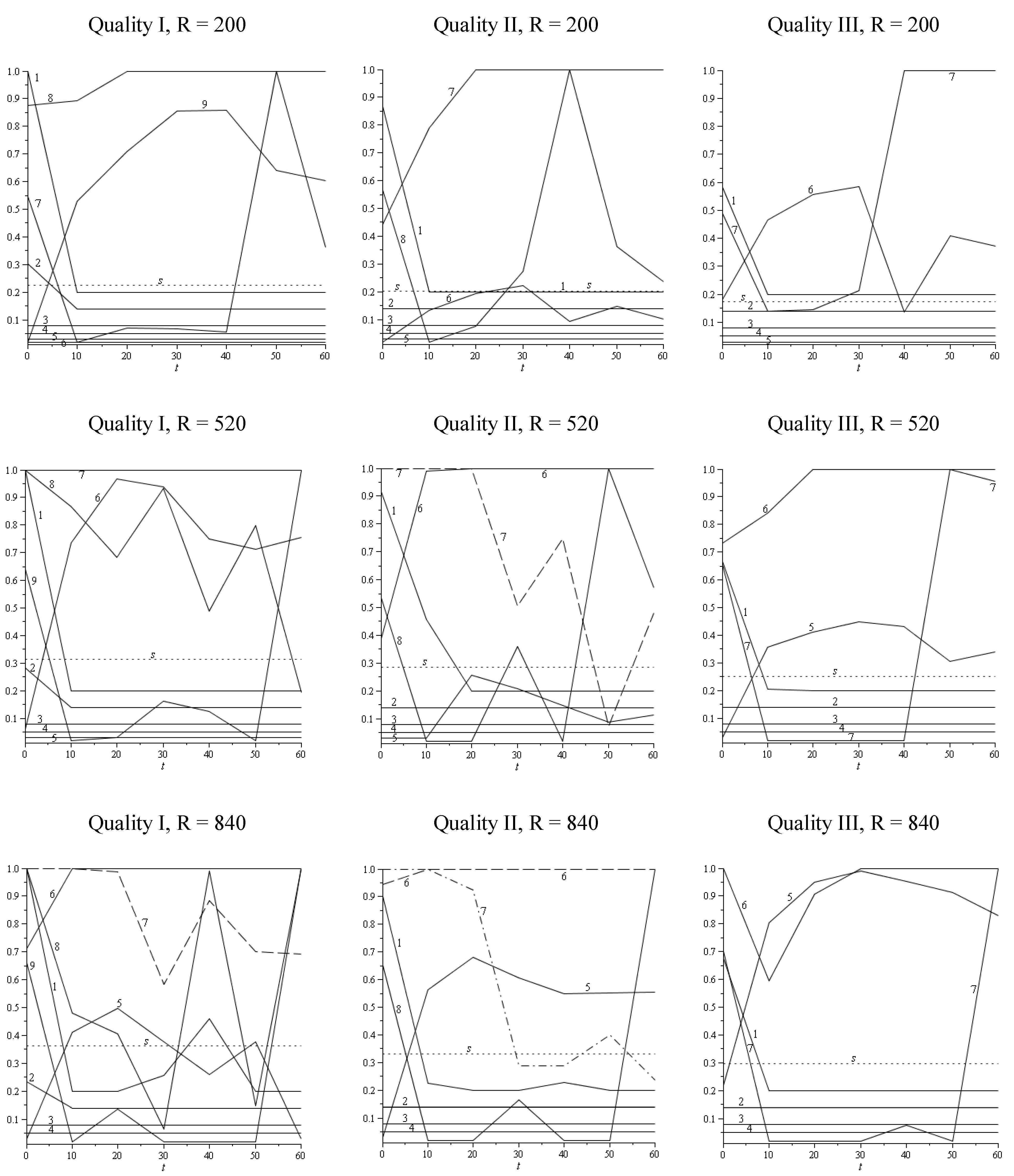
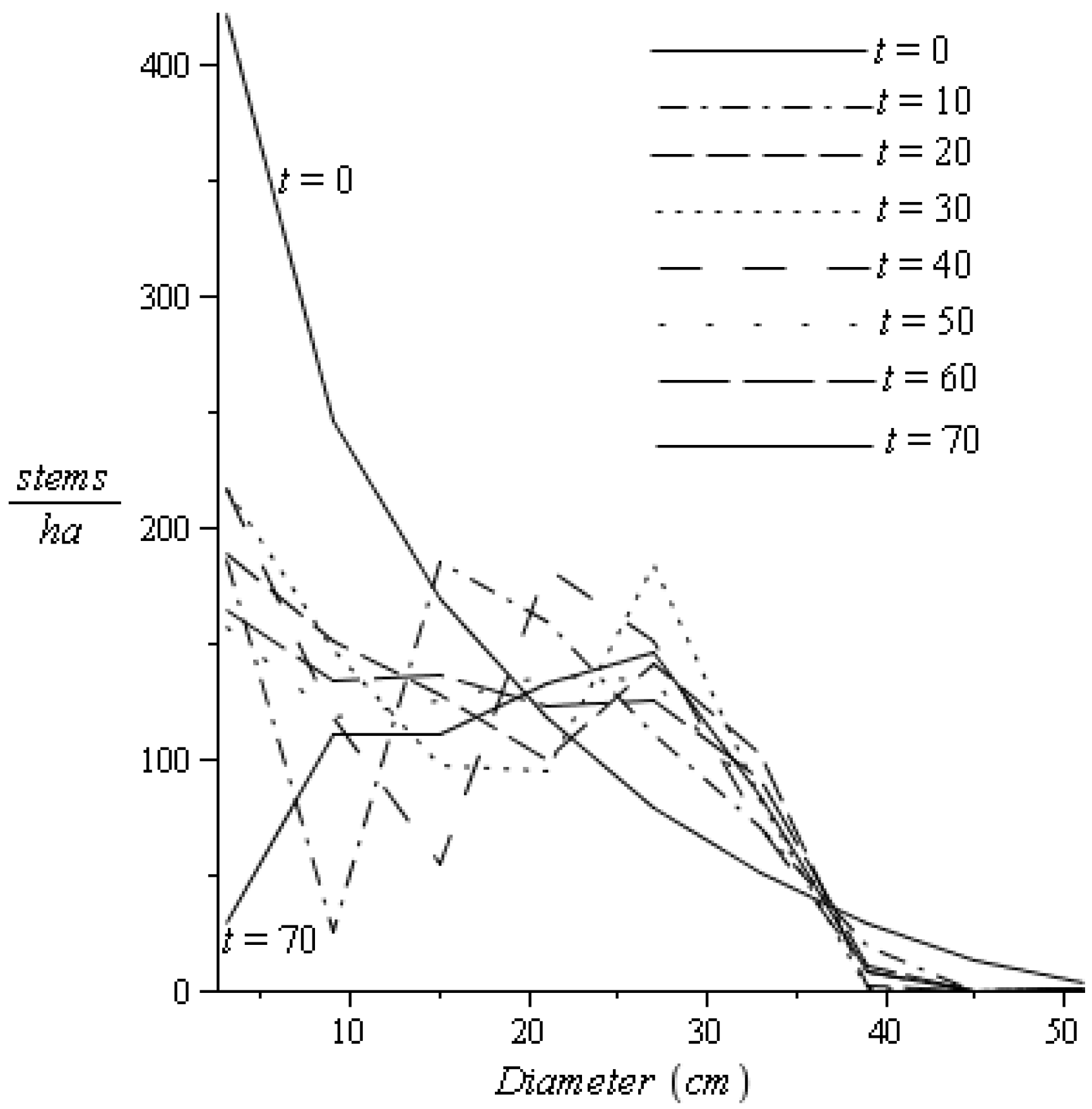
2.3.4. Sustainable/Stable Harvesting Strategy: Stable Diameter Distribution

As shown in the Introduction, the “sustainable/stable” harvesting strategy is aimed at reaching in each harvest the proportions of stems/ha in each class corresponding to the stable diameter distribution of the stand, yielding the following “sustainable/stable” harvest rate:
Forests 04 00830 i007
for all the diameter classes and time steps (s also includes the natural mortalities). This rate corresponds to the case in which the right eigenvector associated with the dominant eigenvalue λ = 1 of the transition matrix with harvests is W0.
As commented on in Section 2.2, by applying the “sustainable/stable” harvesting strategy to each scenario and setting X(0) = W0 (stable diameter distribution) as the initial condition, the basal area of the stand continuously oscillates between the Gmin (after harvesting) and Gmax (before harvesting) values, and the stable diameter distribution is reached at each time step. The calculations for the 27 scenarios of this study, obtained by combining three levels of diameter growth with three levels of recruitment (R = 200, 520 or 840 stems/ha) and three levels of stand basal area (G = Gmax = 22, 24 or 26 m2/ha) are shown in Table 2 along with the population growth rates, λ0, the “sustainable/stable” harvest rates, s, and the minimum basal areas, Gmin.
The results obtained for λ0 are within the intervals corresponding to other tree species. In this regard, Ramula and Lehtilä [28] and Zuidema [29] summarize the main characteristics of matrix models, for 35 woody species in the first case and for 37 plant species (13 of them trees) in the second. The variation range for λ0 went from 0.977 to 1.589 in the first case and from 0.826 to 2.334 in the second. In natural forests, with light or no human intervention, λ0 values are much lower, because of competition, which increases mortality rates and reduces transition probabilities, as well as recruitment. However, our results for λ0, still within the intervals given in [28] and [29], were expected to be slightly high, due to the fact that natural mortalities were absorbed by the harvesting rate, h, not being incorporated into matrix A.
Table 2. Numerical values for λ0, s, stable distributions and NPV0 (R, recruitment; Q I–III, quality class I–III; λ0, population growth rate without harvests; s, stable harvest rate; G, basal area in m2/ha; Est. Dis., stable diameter distribution in stem/ha; NPV0, net present value under the stable equilibrium in €/ha for i = 3%).
R = 200 stem/haR = 520 stem/haR = 840 stem/ha
Q IG = 22λ01.3050911.4776711.594240
s0.2337700.3232590.372742
Gmin16.85706814.88829613.799677
Est. Dis.[186.1, 122.9, 96.4, 77.2, 61.4, 47.5, 34.6, 22.1, 7.2][416.9, 239.8, 162.6, 110.9, 73.4, 45.7, 25.5, 11.4, 2.4][615.9, 325.9, 202.3, 125.4, 74.6, 41.1, 19.8, 7.4, 1.2]
NPV05,347.366,118.036,383.55
G = 24λ01.2924991.4589591.571264
s0.2263050.3145800.363570
Gmin18.56868516.45008115.274322
Est. Dis.[188.3, 125.7, 99.8, 81.0, 65.4, 51.4, 38.3, 25.3, 8.6][423.2, 246.9, 169.9, 117.8, 79.4, 50.5, 28.9, 13.4, 2.9][626.4, 336.8, 212.6, 134.2, 81.5, 45.9, 22.7, 8.8, 1.5]
NPV05,743.336,611.136,918.95
G = 26λ01.2813051.4423421.550881
s0.2195460.3066830.355205
Gmin20.29180818.02624116.764668
Est. Dis.[190.3, 128.3, 102.9, 84.5, 69.1, 55.3, 42.0, 28.5, 10.1][429.0, 253.5, 176.8, 124.3, 85.3, 55.3, 32.4, 15.5, 3.5][636.1, 347.0, 222.4, 142.6, 88.2, 50.8, 25.7, 10.2, 1.9]
NPV06,130.457,096.297,447.43
Q IIG = 22λ01.2620931.4125271.514472
s0.2076650.2920490.339704
Gmin17.43136915.57491914.526515
Est. Dis.[233.3, 147.0, 113.7, 90.3, 71.1, 53.9, 37.2, 16.6][516.1, 280.5, 185.4, 123.4, 79.1, 46.6, 23.0, 6.5][757.0, 376.4, 226.4, 135.8, 77.3, 39.6, 16.4, 3.7]
NPV04,239.224,986.615,284.13
G = 24λ01.2511401.3961881.494358
s0.2007290.2837640.330816
Gmin19.18250917.18965616.060414
Est. Dis.[236.3, 150.7, 118.0, 95.0, 76.1, 58.9, 41.9, 19.5][524.6, 289.4, 194.4, 131.7, 86.1, 52.0, 26.5, 7.8][771.0, 389.9, 238.8, 146.1, 85.0, 44.7, 19.1, 4.5]
NPV04,542.735,373.955,710.91
G = 26λ01.2414061.3816841.476521
s0.1944620.2762450.322732
Gmin20.94398918.81762117.608961
Est. Dis.[239.1, 154.0, 122.0, 99.5, 80.9, 63.8, 46.6, 22.6][532.4, 297.7, 202.8, 139.6, 93.0, 57.4, 30.1, 9.2][783.9, 402.5, 250.5, 156.0, 92.7, 49.8, 22.0, 5.4]
NPV04,838.925,754.146,131.06
Q IIIG = 22λ01.2206041.3508161.439536
s0.1807330.2597070.305332
Gmin18.02386616.28645415.282699
Est. Dis.[295.4, 179.0, 138.1, 110.0, 86.7, 64.6, 32.8][644.2, 332.8, 216.0, 140.9, 87.0, 46.5, 14.8][937.6, 440.2, 257.8, 149.7, 80.5, 36.1, 9.2]
NPV03,202.563,906.484,224.82
G = 24λ01.2111641.3366301.422004
s0.1743480.2518500.296767
Gmin19.81565117.95561116.877591
Est. Dis.[299.6, 183.8, 143.8, 116.4, 93.7, 71.8, 38.0][655.8, 344.3, 227.4, 151.3, 95.6, 52.8, 17.6][956.3, 457.2, 273.0, 162.1, 89.4, 41.4, 11.0]
NPV03,421.694,194.954,548.76
G = 26λ01.2027801.3240441.406468
s0.1685930.2447380.288999
Gmin21.61658319.63681018.486024
Est. Dis.[303.4, 188.3, 149.1, 122.5, 100.4, 79.0, 43.6][666.3, 355.0, 238.2, 161.4, 104.2, 59.2, 20.4][973.6, 473.1, 287.6, 174.1, 98.3, 46.9, 12.9]
NPV03635.054477.234866.59
The NPV values corresponding to the “sustainable/stable” harvesting strategies are:
Forests 04 00830 i008
Since the optimal harvesting strategies produced by the solutions of the discrete optimal control problem described in Section 2.2 could give rise to diameter distributions (X) that differ from the stable (W0), we evaluated the distance between these distributions with Keyfitz’s Δ:
Forests 04 00830 i009
where xi and wi are the components of the diameter distributions X and W0, scaled to one [30]:
Forests 04 00830 i010
The maximum value of Δ is one, and the minimum of zero occurs when the diameter distributions, X and W0 (scaled to one), are identical. Smaller values of Δ result when the distributions, X and W0 (scaled to one), become more similar.

2.3.5. Stumpage Value Model

The stumpage value model applied in this study is a generalization of the model proposed for Quality I in [14] for Pinus nigra in the Spanish Iberian System. In Table 3, we provide the stumpage prices we used in the objective function. Industrial destinations and diameter classes considered are based on those used in previous studies [27,31]. The regression models adjusted to these data appear in Figure 2. The prices in Table 3 come from the official statistics [32] and have been contrasted with real data from actual harvests. The stumpage prices of Pinus nigra in Spain have remained fairly stable between 1994 and 2011 [32].
Table 3. Stumpage prices (€/m3) of Pinus nigra in Spain according to diameter class and contribution to the final price of the four industrial destinations considered.
ProductsDiameter classes (cm)
<2020–40 >40
Particle board61.20.6
Poles011.850
Sawlog09.811.76
High quality sawlog009.96
Total average price622.8522.32
Figure 2. Stumpage price models: Quality I, v = D3.186471 exp(−7.704952 − 8.678687∙10−3 D); Quality II, v = D3.114196 exp(−7.476506 − 9.903125∙10−3 D); and Quality III: v = D2.987053exp(−7.110977 − 1.078752∙10−2D) (stumpage prices v in euro stem−1 and diameter D in cm). The coefficient of determination was always greater than 0.9999.
Forests 04 00830 g002
The last row in Table 3 shows average price per cubic meter for trees belonging to the different diameter classes. This price is obtained by adding up the four rows above showing the contributions to the final value of a tree of the four industrial destinations according to the percentage of wood of each diameter class going into each product type. The prices of particle board, poles, sawlog and high quality sawlog are 6.0, 39.5, 19.6 and 33.2 €/m3, respectively.

3. Results and Discussion

3.1. Results

By substituting the transition probabilities in Table 1, the “sustainable/stable” harvest rates, s, and stable diameter distributions, W0, in Table 2, into the proposed discrete optimal control model and solving globally the corresponding optimization problems (Solver finds the globally optimal solution to each problem by changing the hk(t) variables, for k = 1, 2, … , n, and t = 0, 10, 20, … , 70 years), we obtained optimal state and control variables, xk(t) and hk(t); basal areas before and after each harvest; optimal NPV and the NPV corresponding to the “sustainable/stable” harvesting strategy; and Keyfitz’s Δ for all the scenarios. The discount rates applied fell between 2%6%, as is typical of forest management studies.
We thus obtain four main results. First, Figure 3 shows the population dynamics, xk, needed to maximize the NPV function over 70 years with G = 24 m2 ha−1 and i = 3%. Second, Figure 4 depicts the optimal harvesting strategies, hk(t), for G = 24 m2 ha−1 and i = 3%. Third, the NPV increase between the “sustainable/stable” harvesting strategy s and the optimal harvesting strategy (maximizing NPV function) for i = 3% and different values of Quality, R and G, appears in Table 4. Fourth, Table 5 shows the set of values for Keyfitz’s Δ at the end of the harvest cycle, along with the population growth rate, λT, for the whole harvest cycle of T = 70 years. Note that the transition matrix, AT, for the whole harvest cycle (from t = 0 to t = 70 years) is:
Forests 04 00830 i011
and that λT < 1 for all the scenarios. Therefore, the economically optimal harvesting strategies were unsustainable for all the scenarios, which implies that, by executing the same harvest cycle indefinitely, the population of trees would be decaying until extinction.
The tables and figures mentioned in the above paragraph are included below.
The optimal harvesting strategy, designed to maximize NPV, results in higher NPV figures than the “sustainable/stable” strategy. For i = 3%, this increment is always greater than 8.43%, with a maximum of 17.50% for Quality I, R = 520 stems/ha and G = 22 m2/ha. The NPV increase was greater for Quality I than for Quality II or Quality III. For higher discount rates, NPV increase rates are slightly higher, from a minimum of 10.88% to a maximum of 21.29% for i = 6%, Quality I, R = 520 stems/ha and G = 24 m2/ha. The pattern of change for the three site qualities is kept for the different discount rates.
Figure 3. Population dynamics, xk, to maximize the NPV function throughout a harvest cycle of 70 years for G = 24 m2 ha−1 and i = 3% (left: Quality I; middle: Quality II; right: Quality III; first row: R = 200 stems/ha; second row: R = 520 stems/ha; third row: R = 840 stems/ha). The initial conditions (intercepts on ordinate axis) are defined by the stable diameter distributions.
Forests 04 00830 g003
Figure 4. Optimal harvesting strategies, hk(t), for G = 24 m2 ha−1 and i = 3% (left: Quality I; middle: Quality II; right: Quality III; first row: R = 200 stems/ha; second row: R = 520 stems/ha; third row: R = 840 stems/ha). The dashed lines depict the “sustainable/stable” harvest rates, s.
Forests 04 00830 g004
Table 4. Optimal strategy NPV and NPV increase (%) between the optimal and “sustainable/stable” harvesting strategies for i = 3% and different levels of Quality, R and G (G in m2/ha).
R = 200 stem/haR = 520 stem/haR = 840 stem/ha
NPV
(€/ha)
NPV
increase (%)
NPV
(€/ha)
NPV
increase (%)
NPV
(€/ha)
NPV
increase (%)
Q IG = 226205.0716.047188.4917.507468.1817.00
G = 246636.6515.557767.2917.498095.4317.00
G = 267056.8015.118316.4417.198718.0017.06
Q IIG = 224788.2112.955754.8315.406139.0516.18
G = 245124.0712.806203.8315.446623.8015.99
G = 265453.9612.716647.7715.537098.1415.77
Q IIIG = 223,502.949.384,389.2712.364,820.6514.10
G = 243,724.858.864,701.4812.075,185.9714.00
G = 263,941.588.435,007.2411.845,529.3513.62
Table 5. Keyfitz’s Δ values, corresponding to the distance between the diameter distribution associated with the optimal harvesting strategy (for t = 70 years) and the stable diameter distribution (W0), as well as population growth rates, λT, for the whole harvest cycle (from t = 0 to t = 70 years) (G in m2/ha).
R = 200 stem/haR = 520 stem/haR = 840 stem/ha
ΔλTΔλTΔλT
Q IG = 220.4504150.0560330.3973110.0026020.3946240.000226
G = 240.4343040.1787540.3928130.0028660.3902070.000284
G = 260.4252440.2105730.4372350.0028660.3872820.000559
QIIG = 220.4677450.3105560.4902250.0066280.3619890.004161
G = 240.4679350.3337050.4876510.0110890.3519670.004161
G = 260.4683820.3541820.4780310.0149210.3469970.004161
Q IIIG = 220.3482970.6040920.3925340.2758170.3359040.365103
G = 240.4228800.5511020.3853670.3034780.3233090.336591
G = 260.4177560.5624000.3789340.3375220.3245590.312709
Applying the optimal harvesting strategy, for Qualities I, II and III, the diameter distribution of the stand evolved through time, leaving the initial equilibrium distribution and tending toward a diameter distribution more characteristic of even-aged stands. For high recruitments (R = 840 stems/ha), the resulting distribution at the end of T = 70 years is a bimodal distribution, more accentuated for Quality I. Figure 5 contains, as an example, a scenario corresponding to Quality I, G = 24 m2/ha, R = 520 stems/ha and i = 3%.
Figure 5. Evolution of the diameter distribution with the economically optimal harvesting strategy throughout a harvest cycle of 70 years for Quality I, G = 24 m2/ha, R = 520 stems/ha and i = 3%.
Forests 04 00830 g005
The influence of small variations in the discount rate or the natural mortality rates on the optimal harvesting strategies was minimal, because they did not change the general pattern of the solutions.

3.2. Discussion and Conclusions

This study proposes a model that combines an objective function comprising the NPV of all the management operations in a planning horizon of 70 years with a matrix model for the population dynamics. The resulting discrete optimal control model provides a simple tool for heuristic analysis to answer the “what if” questions in relation to forest management actions.
Following López et al. [7,8,9], we calculated the transition probabilities considering that pk is an average global property shared by all the individuals in the same class k, and that, given the basal area constraints and the low basal area scenarios of this study, there is a low variability around the mean pk values (see Section 2.3.1) thus resulting in a small influence on diameter growth. Moreover, in the case of these constrained optimization matrix models, in which the search for optimal paths throughout the phase space is mainly governed by the objective function, optimal decisions are essentially conditioned by the stumpage prices, i.e. by selective harvesting, and thus stand density has minor influence on the objective.
López et al. [8] also show that results obtained for λ0 are sensitive to the width, w, of the diameter classes, such that the most conservative values of λ0 and s result from the lowest values of w (which does not allow an individual tree to jump over more than one diameter class in a single projection). The minimum (integer) widths of the diameter classes compatible with this model assumption were w = 6 cm for Quality I, w = 5 cm for Quality II and w = 4 cm for Quality III. However, since the dominant eigenvalue λ0 and the stable diameter distribution are not substantially affected by small or even moderate changes in the width of the diameter classes, the width considered throughout this study was w = 6 cm, to facilitate the comparison of results.
The basal area indirectly resulted in optimization problems, such as a “bang-bang control” variable, which oscillated between Gmin and Gmax. The upper and lower bounds imposed on basal area values are derived from the “sustainable/stable” harvesting strategy (to compare the optimal strategy with the “sustainable/stable”).
By applying optimal harvesting strategies, the schedules aim for the highest NPV, with an intense harvest (h > 0.5) performed in the diameter classes during the planning horizon as follows:
For high recruitments, the intense harvest applies to the upper diameter class at the beginning (first period) and the end (seventh period) of the planning horizon. In addition, for medium and high recruitments, the intense harvest gets performed in every period of the planning horizon for the diameter classes corresponding to poles, while low recruitments follow a different pattern. In this case, the intense harvest is performed in the upper diameter classes, since low recruitments are associated with a lower number of stems per hectare with a higher average diameter.
For the three qualities, this harvest pattern caused a decrease in the number of stems of the first diameter class, such that at the end of the time horizon, the diameter range of the distribution narrowed and shifted from a reversed J-shaped curve to a bell-shaped curve, centered on the medium diameter classes (18–36 cm), as is typical of an even-aged stand distribution (see Figure 5). The intermediate diameter classes correspond to trees going to the production of poles. This type of evolution might be favored by market conditions for Pinus nigra products in Spain, because of the high price of poles obtained from those diameter classes (see Table 3).
There is not a significant change in the harvest pattern for the optimal strategy when higher discount rates are considered, except for a slight trend to advance harvest in the upper diameter classes. This result, leading to an earlier harvest, is consistent with an increase in the discount rate.
The NPV increase rate between the optimal and “sustainable/stable” harvesting strategies grows slightly with discount rate. The pattern of NPV change for the three site qualities is kept for the different discount rates considered in the analysis.
By applying the optimal harvesting strategies, at the end of T = 70 years, the Keyfitz’s Δ values ranged from 0.32 to 0.49; that is, the stand moved away from the equilibrium. For i = 3%, the lowest Δ values emerged for higher recruitments (R = 840 stems/ha) and Quality III.
Regarding the sustainability of the optimal harvesting strategies, all the scenarios were unsustainable (see Table 5). In fact, the population growth rate, λT, for the whole harvest cycle (given by the dominant eigenvalue of the transition matrix, AT) was always λT < 1. Moreover, the population decline was greater for Quality I, followed by Quality II and Quality III, and with some exceptions, the greater the recruitment was, the greater the population decline induced by the optimal harvesting strategies. It is not difficult to implement constraints to obtain λ = 1 at each time step (for example, by assuming in the model a new set of constraints obtained by solving the determinant det(A(I – H(t)) – I) = 0 for hn(t), at each time step), but this does not guarantee either that λT = 1 or that the stable distribution is reached at t = T (the λT values are in this case closer to one, but clearly, it remains λT < 1 for all the scenarios). However, with the “sustainable/stable” harvesting strategy, we get λ = 1 and the stable diameter distribution at each time step, and λT = 1 for the whole harvest cycle.
In conclusion, the proposed discrete optimal control model was used to analyze if the introduction of an NPV maximizing management strategy on the dynamics of uneven-aged Pinus nigra stands in demographic equilibrium (with the stable diameter distribution W0 set as the initial condition), leads to distributions that move away from that equilibrium through time and assessing the sustainability of those strategies. Our results suggest that the economically optimal harvesting strategies were unsustainable and unstabilizing for all the scenarios. This is unsurprising, because these assumptions (λT = 1 and W0) were not specified in the model. In addition, these considerations in general are not present in previous models to optimize uneven-aged stands management. Therefore, it would be interesting to incorporate into further evolutions of this optimization model constraints related to the maintenance of a certain age structure, a final stable distribution (i.e., X(T) = W0) and/or the sustainability for the whole harvest cycle (λT = 1). These determinants are common in traditional uneven-aged forest management.

Conflicts of Interest

The authors declare no conflict of interest.

References

  1. Buongiorno, J.; Michie, B.R. A matrix model of uneven-aged forest management. For. Sci. 1980, 26, 609–625. [Google Scholar]
  2. Caswell, H. Matrix Population Models: Construction, Analysis, and Interpretation, 2nd ed.; Sinauer Associates Inc.: Sunderland, MA, USA, 2001; p. 713. [Google Scholar]
  3. Picard, N.; Ouédraogo, D.; Bar-Hen, A. Choosing classes for size projection matrix models. Ecol. Model 2010, 221, 2270–2279. [Google Scholar] [CrossRef]
  4. Escalante, E.; Pando, V.; Ordoñez, C.; Bravo, F. Multinomial logit estimation of a diameter growth matrix model of two Mediterranean pine species in Spain. Ann. For. Sci. 2011, 68, 715–726. [Google Scholar] [CrossRef]
  5. Gotelli, N.J. A Primer of Ecology; Sinauer Associates Inc.: Sunderland, MA, USA, 2001; p. 265. [Google Scholar]
  6. Schütz, J.P. Modelling the demographic sustainability of pure beech plenter forests in Eastern Germany. Ann. For. Sci. 2006, 63, 93–100. [Google Scholar] [CrossRef]
  7. López, I.; Ortuño, S.F.; Martín, A.J.; Fullana, C. Estimating the sustainable harvesting and the stable diameter distribution of European beech with projection matrix models. Ann. For. Sci. 2007, 64, 593–599. [Google Scholar] [CrossRef]
  8. López, I.; Fullana, C.; Ortuño, S.F.; Martín, A.J. Choosing Fagus sylvatica L. matrix model dimension by sensitivity analysis of the population growth rate with respect to the width of the diameter classes. Ecol. Model 2008, 218, 307–314. [Google Scholar] [CrossRef]
  9. López, I.; Ortuño, S.; García, F.; Fullana, C. Is De Liocourt’s distribution stable? Forest Sci. 2012, 58, 34–46. [Google Scholar] [CrossRef]
  10. Haight, R.G. A comparison of dynamic and static economic models of uneven-aged stand management. Forest Sci. 1985, 31, 957–974. [Google Scholar]
  11. Sethi, S.P.; Thompson, G.L. Optimal Control Theory: Applications to Management Science and Economics, 2nd ed.; Kluwer Academic Publishers: Dordrecht, The Netherlands, 2000. [Google Scholar]
  12. Kronrad, G.D.; Huang, C.H. Financially optimal thinning and final harvest schedules for loblolly pine plantations on nonindustrial private forestland in east Texas. South J. Appl. For. 2002, 26, 13–17. [Google Scholar]
  13. Tahvonen, O. Optimal harvesting of forest age classes: A survey of some recent results. Math Popul. Stud. 2004, 11, 205–232. [Google Scholar] [CrossRef]
  14. López, I.; Ortuño, S.; Martín, A.J.; Fullana, C. Estimating the optimal rotation age of Pinus nigra in the Spanish Iberian System applying discrete optimal control. For. Syst. 2010, 19, 306–314. [Google Scholar]
  15. Maple, Version 16.0, Maplesoft: Ontario, Canada, 2012.
  16. Front Line Systems Solver Premium Platform. Incline Village, NV, USA, 2008. Available online: http://www.solver.com (accessed on 26 July 2013).
  17. Grande, M.A.; García Abril, A. Los Pinares de Pinus nigra Arn. en España: Ecología, uso y gestión; Fundación Conde del Valle de Salazar (FUCOVASA): Madrid, Spain, 2005; pp. 1–53. [Google Scholar]
  18. Gómez Loranca, J.A. Modelo de crecimiento y producción para Pinus nigra Arn. en el Sistema Ibérico. Revista Montes 1998, 54, 5–18. [Google Scholar]
  19. Siegel, W.; Hoover, W.; Haney, H.; Liu, K. Forest Owners’ Guide to the Federal Income Tax; Agriculture Handbook No. 708; United States Department of Agriculture, Forest Service: Washington, DC, USA, 1995; p. 138. [Google Scholar]
  20. Retana, J.; Espelta, J.M.; Habrouk, A.; Ordóñez, J.L.; Solà-Morales, F. Regeneration patterns of three Mediterranean pines and forest changes after a large wildfire in north-eastern Spain. Ecoscience 2002, 9, 89–97. [Google Scholar]
  21. Tíscar, P.A. Dinámica de regeneración de Pinus nigra subs. Salzmannii al sur de su área de distribución: etapas, procesos y factores implicados. Inv. Agrar. Sist. Rec. F. 2007, 16, 124–135. [Google Scholar]
  22. Tíscar Oliver, P.A.; Lucas, M.E.; Tíscar Soria, M.A. La alteración del suelo y la espesura como factores de regeneración de Pinus nigra subs. Salzmannii a lo largo de su área de distribución. Revista Montes 2010, 103, 10–15. [Google Scholar]
  23. Schütz, J.P. Le régime du jardinage. Document autographique du cours de Sylviculture III; Chaire de Sylviculture; E.T.H. Zürich: Zürich, Switzerland, 1989; p. 55. [Google Scholar]
  24. Serrada, R.; Domínguez Lerena, S.; Sánchez Resco, M.I.; Ruiz Ortiz, J. El problema de la regeneración natural de Pinus nigra Arn. Revista Montes 1994, 36, 52–57. [Google Scholar]
  25. Van Mantgem, P.J.; Stephenson, N.T. The accuracy of matrix population model projections for coniferous trees in the Sierra Nevada, California. J. Ecol. 2005, 93, 737–747. [Google Scholar] [CrossRef]
  26. Misir, M.; Misir, N.; Yavuz, H. Modeling individual tree mortality for Crimean pine plantations. J. Environ. Biol. 2007, 28, 167–172. [Google Scholar]
  27. Trasobares, A.; Pukkala, T. Optimising the management of uneven-aged Pinus sylvestris L. and Pinus nigra Arn. mixed stands in Catalonia, north-east Spain. Ann. For. Sci. 2004, 61, 747–758. [Google Scholar] [CrossRef]
  28. Ramula, S.; Lehtilä, K. Matrix dimensionality in demographic analyses of plants: When to use smaller matrices? Oikos 2005, 111, 563–573. [Google Scholar] [CrossRef]
  29. Zuidema, P.A. Demography of Exploited Tree Species in the Bolivian Amazon; PROMAB Scientific Series 2; Promab: Riberalta, Bolivia, 2000; p. 240. [Google Scholar]
  30. Keyfitz, N. Introduction to the Mathematics of Population; Addison-Wesley: Reading, MA, USA, 1968; p. 464. [Google Scholar]
  31. Montero, G.; Rojo, A.; Alía, R. Determinación del turno de Pinus sylvestris L en el Sistema Central. Revista Montes 1992, 29, 42–47. [Google Scholar]
  32. Boletín Mensual de Estadística 1994–2011; Ministerio de Agricultura, Alimentación y Medio Ambiente: Madrid, Spain, 2011; pp. 29–33.

