Deforestation and Changes in Landscape Patterns from 1979 to 2006 in Suan County, DPR Korea


Abstract
:1. Introduction
2. Materials and Methods
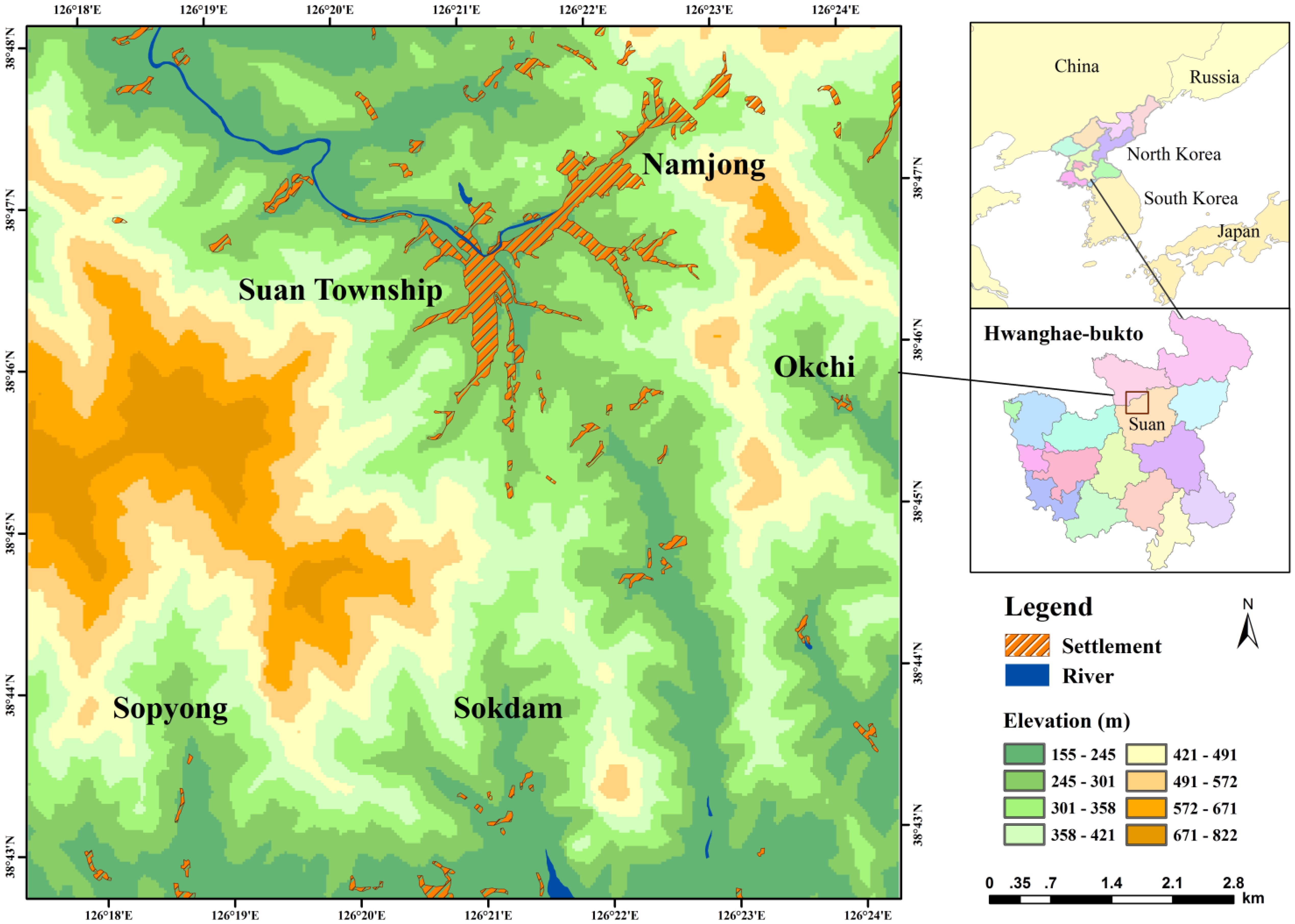
2.1. Study Area

2.2. Data Acquisition and Preprocessing
2.3. Land Classification System
2.4. Land-Cover Classification
2.5. Accuracy Assessment
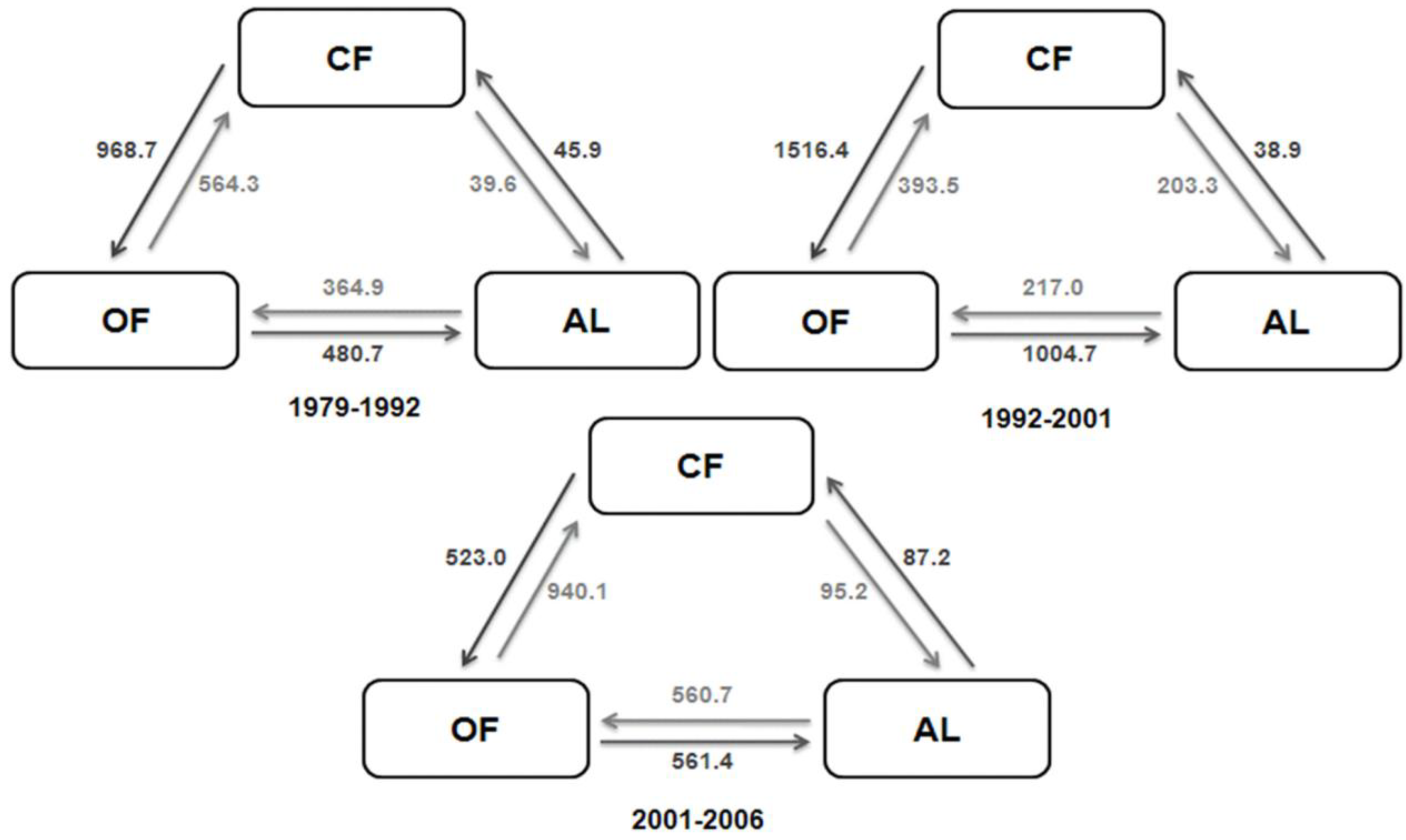
2.6. Land-Cover Change Detection
2.7. Landscape Pattern Analysis
3. Results
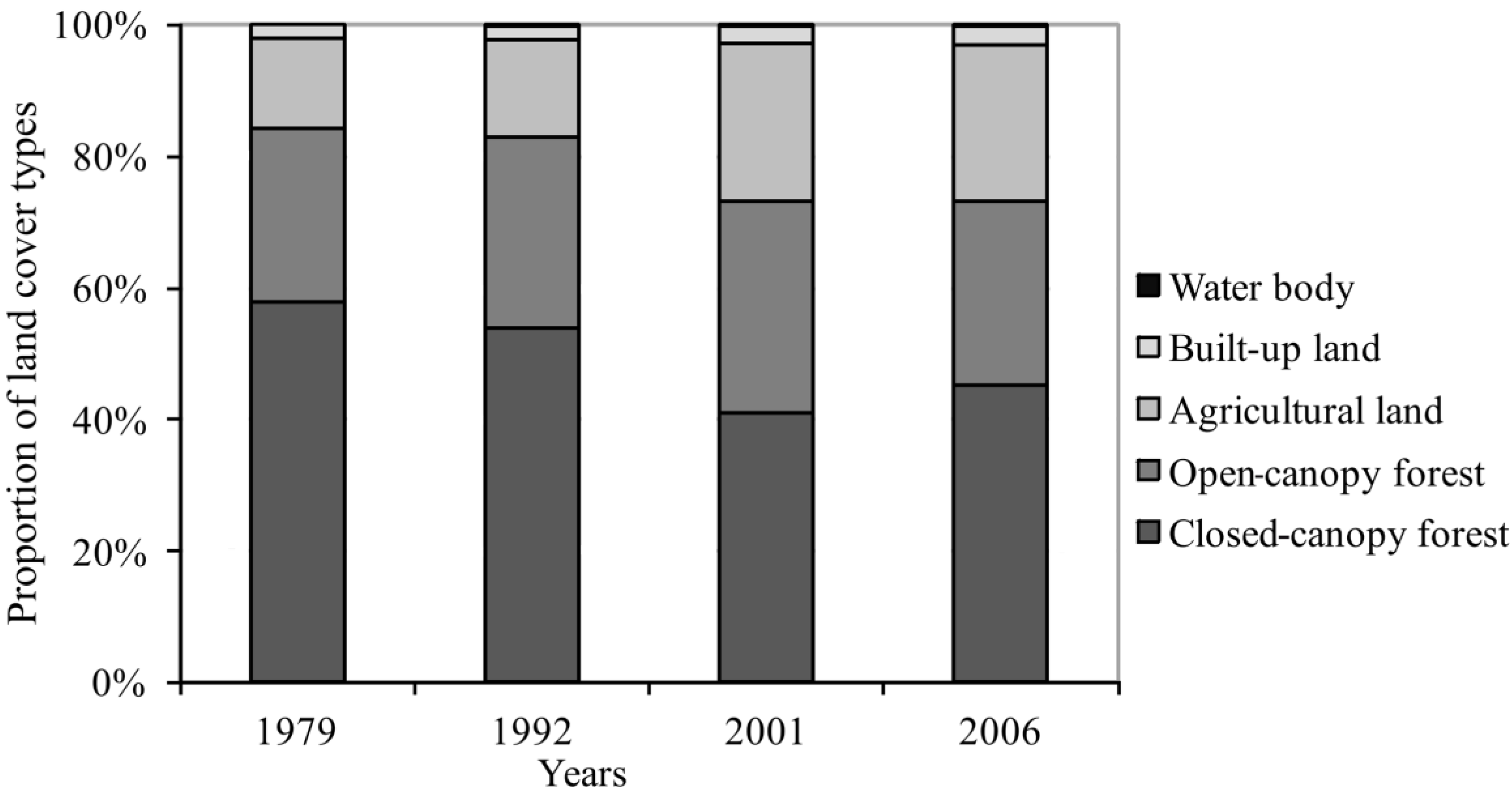
3.1. Land-Cover Trends

| Index | Description (McGarigal and Marks 1995; de Barros Ferraz, 2009) | Unit |
|---|---|---|
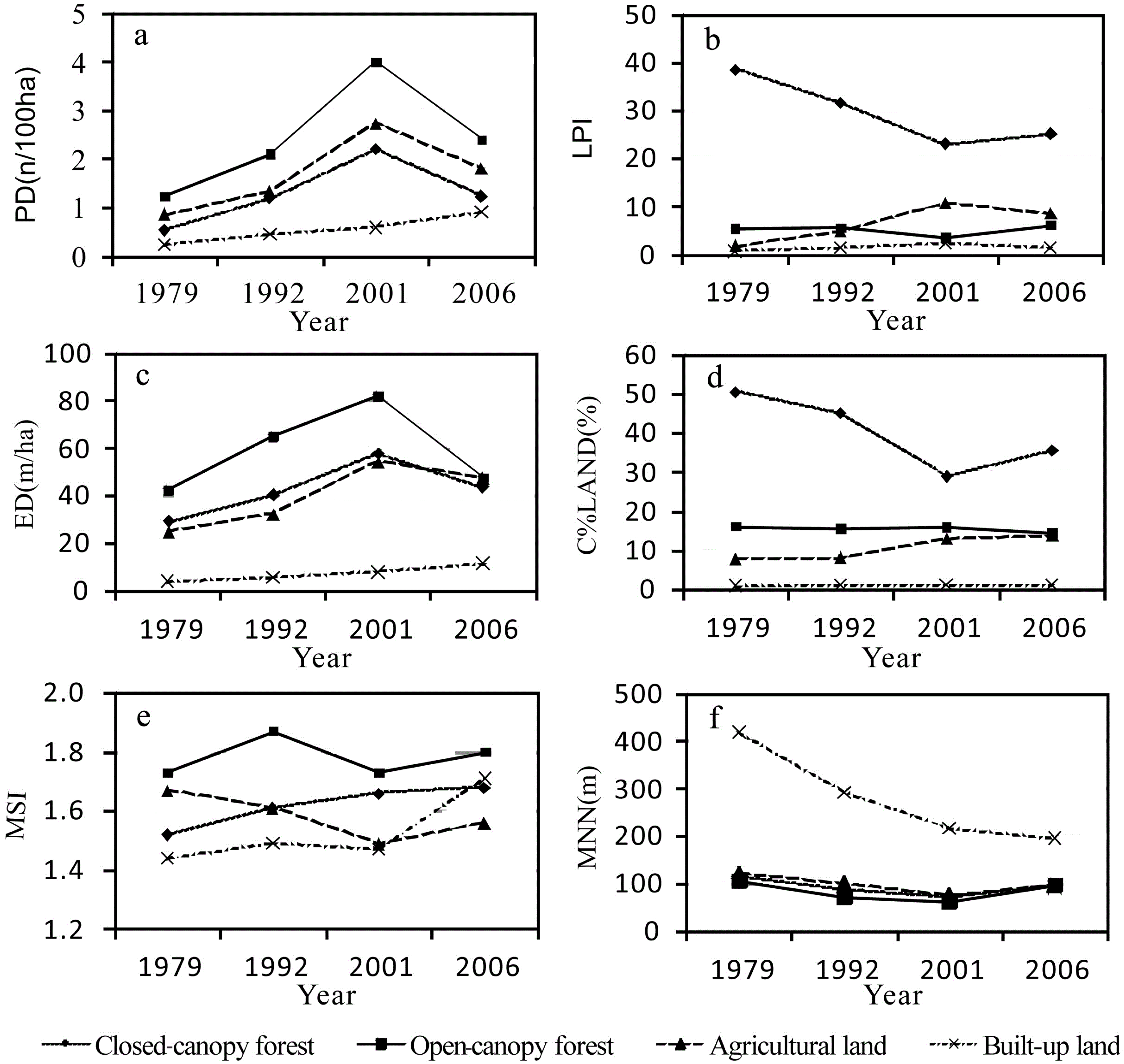
| PD | Patch density—density of patches for each land-use (number of patches per unit of area), representing an aspect of fragmentation: dissection of patches. Higher values represent a more fragmented landscape | N/100ha |
| ED | Edge density—standardized edge to a per unit area basis that facilitates comparisons among landscapes of varying size | m/ha |
| LPI | Largest Patch Index—proportion of the landscape occupied by the largest patch of each land use, representing another aspect of fragmentation: patch dominance. Values range from 0 (no patches) to 100 (1 patch occupying the entire landscape) | % |
| C%LAND | Core area percentage of landscape—the core area in each patch type as a percentage of total landscape area | % |
| MSI | Mean shape index—the average patch shape, or the average perimeter-to-area ratio, for a particular patch type (class) or for all patches in the landscape | - |
| MNN | Mean nearest neighbor distance—mean distance between patches of same class (land-use), which could represent another aspect of fragmentation: connectivity between patches. Values range from 0 (adjacent patches) to infinity | m |


| Class | 1979–1992 | 1992–2001 | 2001–2006 | 1979–2006 | ||||
|---|---|---|---|---|---|---|---|---|
| ha a−1 | % | ha a−1 | % | ha a−1 | % | ha a−1 | % | |
| Closed canopy forest | −30.57 | −6.89 | −142.88 | −23.97 | 82.74 | 10.14 | −47.02 | −20.72 |
| Open canopy forest | 20.48 | 10.14 | 36.19 | 11.26 | −84.16 | −13.07 | 6.34 | 8.33 |
| Agriculture land | 7.84 | 7.34 | 99.86 | 60.29 | −5.30 | −1.11 | 36.08 | 66.52 |
| Built-up land | 1.72 | 11.11 | 6.92 | 27.78 | 6.84 | 11.94 | 4.40 | 50.83 |
| Water | 0.52 | - | −1.33 | −0.8 | −0.14 | −12.12 | 0.19 | - |

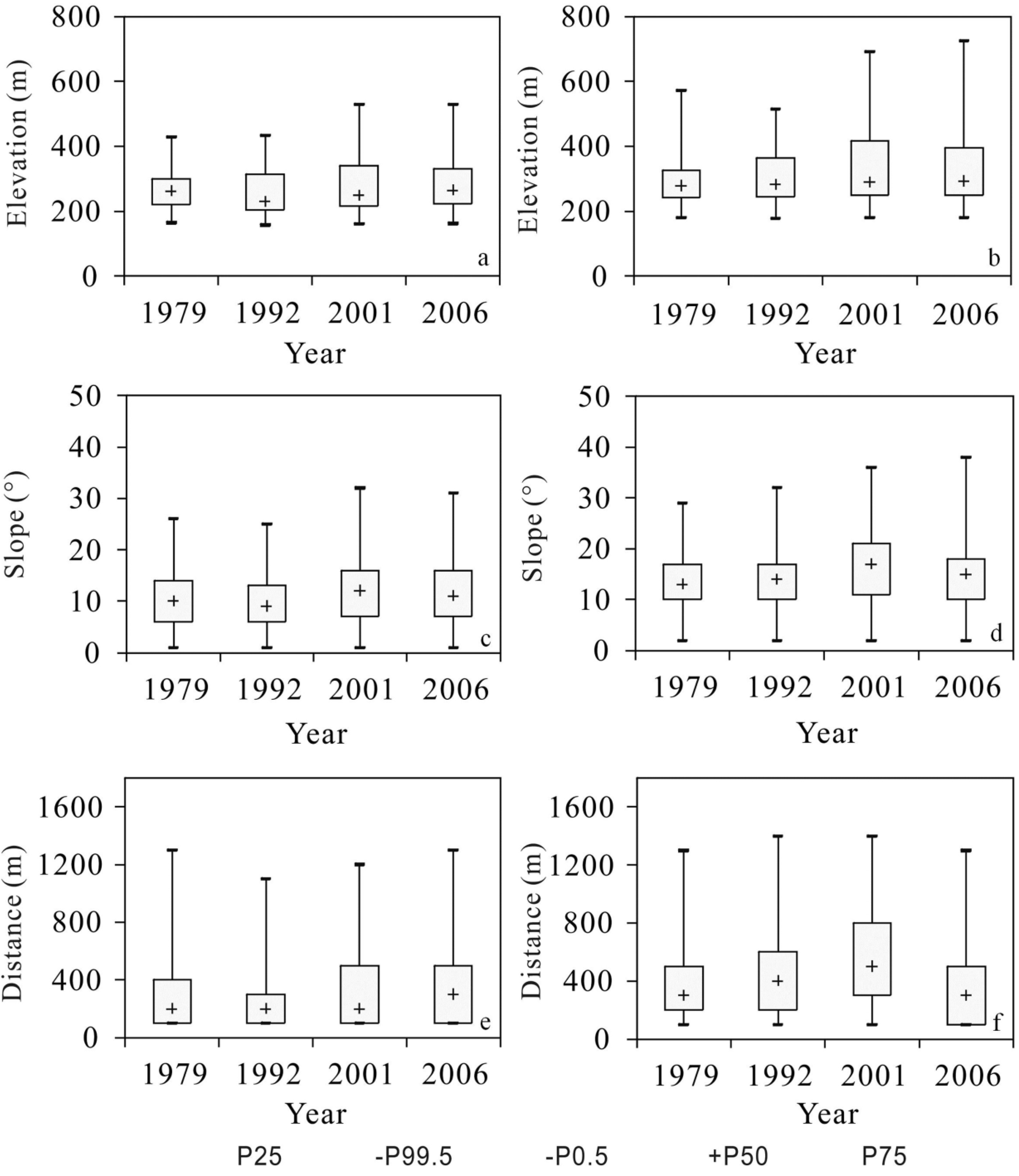
3.2. Spatial Analysis
3.3. Landscape Structure Dynamics


4. Discussion
4.1. Deforestation and Drivers
4.2. Landscape Fragmentation
4.3. Forest Transition and Livelihood Development
5. Conclusions
Acknowledgements
Conflicts of Interest
References
- Williams, M. Dark ages and dark areas: Global deforestation in the deep past. J. Hist. Geog. 2000, 26, 28–46. [Google Scholar] [CrossRef]
- Food and Agriculture Organization of the United Nations, Global Forest Resources Assessment 2010; Main report; Food and Agriculture Organization of the United Nations: Rome, Italy, 2010.
- Smith, J.; Obidzinski, K.; Subarudi; Suramenggala, I. Illegal logging, collusive corruption and fragmented governments in Kalimantan, Indonesia. Int. For. Rev. 2003, 5, 293–302. [Google Scholar]
- Morton, D.C.; DeFries, R.S.; Shimabukuro, Y.E.; Anderson, L.O.; Arai, E.; del Bon Espirito-Santo, F.; Freitas, R.; Morisette, J. Cropland expansion changes deforestation dynamics in the southern Brazilian Amazon. Proc. Natl. Acad. Sci. USA 2006, 103, 14637–14641. [Google Scholar] [CrossRef]
- Pfaff, A.; Pfaff, S.P. What drives deforestation in the Brazilian Amazon? Evidence from Satellite and socioeconomic data. J. Environ. Econ. Manag. 1999, 37, 26–43. [Google Scholar] [CrossRef]
- Helgesen, G.; Christensen, N.H. North Korea 2007—Assisting Development and Change; Nordic Institute of Asian Studies, Norwegian Ministry of Foreign Affairs: Oslo, Norway, 2007. [Google Scholar]
- United Nations Environment Programme, DPR Korea: State of the Environment 2003; United Nations Environment Programme, Regional Resource Centre for Asia and the Pacific (UNEP RRC.AP): Bangkok, Thailand, 2003.
- Hayes, P. Unbearable legacies: The politics of environmental degradation in North Korea. Asia Pac. J. 2009, 41, 1–9. [Google Scholar]
- Williams, J.H.; von Hippel, D.; Hayes, P. Fuel and Famine: Rural Energy Crisis in the Democratic People’s Republic of Korea; Policy Paper; Institute on Global Conflict and Cooperation, University of California: San Diego, CA, USA, March 2000. [Google Scholar]
- Food and Agriculture Organization of the United Nations, State of the World’s Forest 2007; Food and Agriculture Organization of the United Nations: Rome, Italy, 2007.
- Lambin, E.F.; Turner, B.L.; Geista, H.J.; Agbolac, S.B.; Angelsend, A.; Brucee, J.W.; Coomesf, O.T.; Dirzog, R.; Fischerh, G.; Folke, C. The causes of land-use and land-cover change: Moving beyond the myths. Glob. Environ. Chang. 2001, 11, 261–269. [Google Scholar] [CrossRef]
- Miles, L.; Kapos, V. Reducing greenhouse gas emissions from deforestation and forest degradation: Global land use implications. Science 2008, 320, 1454–1455. [Google Scholar] [CrossRef]
- Nepstad, D.C.; Verissimo, A.; Alencar, A.; Nobre, C.; Lima, E.; Lefebvre, P.; Schlesinger, P.; Potter, C.; Moutinho, P.; Mendoza, E.; et al. Large-scale impoverishment of Amazonian forests by logging and fire. Nature 1999, 398, 505–508. [Google Scholar] [CrossRef]
- Willson, A. Forest conversion and land use change in rural Northwest Yunnan, China: A fine-scale analysis in the context of the ‘big picture’. Mt. Res. Dev. 2006, 26, 227–236. [Google Scholar] [CrossRef]
- Xu, J.; van Noordwijk, M.; He, J.; Kim, K.-J.; Jo, R.-S.; Pak, K.-G.; Kye, U.-H.; Kim, J.-S.; Kim, K.-M.; Sim, Y.-N.; et al. Participatory agroforestry development for restoring degraded sloping land in DPR Korea. Agrofor. Syst. 2012, 85, 291–303. [Google Scholar] [CrossRef]
- Global Land Cover Facility. Available online: http://glcf.umiacs.umd.edu/ (accessed on 28, April 2009).
- Food and Agriculture Organization of the United Nations, Survey of Tropical of Forest Cover and Study of Change Processes. In Forestry Paper; Food and Agriculture Organization of the United Nations: Rome, Italy, 1996; p. 130.
- Anderson, J.R.; Hardy, E.E.; Roach, J.T.; Witmer, R.E. A Land Use and Land Cover Classification System for Use with Remote Sensor Data; U.S. Government Printing Office: Washington, DC, USA, 1976; p. 28.
- Yu, H.; Luedeling, E.; Xu, J. Winter and spring warming result in delayed spring phenology on the Tibetan Plateau. Proc. Natl. Acad. Sci. USA 2010, 107, 22151–22156. [Google Scholar] [CrossRef]
- Lu, D.; Mausel, P.; Brondizio, E.; Moran, E. Change detection techniques. Int. J. Remote Sens. 2004, 25, 2365–2407. [Google Scholar] [CrossRef]
- Olson, C.E. Elements of photographic interpretation common to several sensors. Photogramm. Eng. 1960, 26, 651–656. [Google Scholar]
- Wang, Y.Q.; Bonynge, G.; Nugranad, J.; Traber, M.; Ngusaru, A.; Tobey, J.; Hale, L.; Bowen, R.; Makota, V. Remote sensing of mangrove change along the Tanzania coast. Mar. Geod. 2003, 26, 35–48. [Google Scholar] [CrossRef]
- Edwards, G. Image Segmentation, Cartographic Information and Knowledge-Based Reasoning: Getting the Mixture Right. In Proceedings of the IGARSS’90 Symposium, University of Maryland, College Park, MD, USA, 20–24 May 1990.
- Mas, J.F. Monitoring land-cover changes: A comparison of change detection techniques. Int. J. Remote Sens. 1999, 20, 139–152. [Google Scholar] [CrossRef]
- Zou, Y.; Zhao, X.; Zhang, Z.; Zhou, Q. An analysis of dynamic changes of China’s grassland on the basis of RS and GIS. Remote Sens. Land. Resour. 2002, 1, 29–33. [Google Scholar]
- McGarigal, K.; Marks, B. FRAGSTATS: Spatial Pattern Analysis Program for Quantifying Landscape Structure; U.S. Department of Agriculture, Forest Service, Pacific Northwest Research Station: Portland, OR, USA, 1995; p. 122. [Google Scholar]
- United Nations Framework Convention on Climate Change, Investment and Financial Flows to Address Climate Change; United Nations Framework Convention on Climate Change: Bonn, Germany, 2007; p. 81.
- Fitzsimmons, M. Effects of deforestation and reforestation on landscape spatial structure in boreal Saskatchewan, Canada. For. Ecol. Manag. 2003, 174, 577–592. [Google Scholar] [CrossRef]
- Armenteras, D.; Gast, F.; Villareal, H. Andean forest fragmentation and the representativeness of protected natural areas in the eastern Andes, Colombia. Biol. Conserv. 2003, 113, 245–256. [Google Scholar] [CrossRef]
- Echeverria, C.; Coomes, D.; Salas, J.; Rey-benayas, J.M.; Lara, A.; Newton, A. Rapid deforestation and fragmentation of Chilean temperate forests. Biol. Conserv. 2006, 130, 481–494. [Google Scholar] [CrossRef]
- Gratkowski, H.J. Wind throw around staggered settings in old-growth Douglas fir. For. Sci. 1956, 2, 60–74. [Google Scholar]
- Ranney, J.; Bruner, M.; Levenson, J. The Importance of Edge in the Structure and Dynamics of Forest Islands. In Forest Islands Dynamics in Man-dominated Landscapes; Burgess, R., Sharpe, D., Eds.; Springer: New York, NY, USA, 1981; pp. 67–95. [Google Scholar]
© 2013 by the authors; licensee MDPI, Basel, Switzerland. This article is an open access article distributed under the terms and conditions of the Creative Commons Attribution license (http://creativecommons.org/licenses/by/3.0/).
Share and Cite
Pang, C.; Yu, H.; He, J.; Xu, J. Deforestation and Changes in Landscape Patterns from 1979 to 2006 in Suan County, DPR Korea. Forests 2013, 4, 968-983. https://doi.org/10.3390/f4040968
Pang C, Yu H, He J, Xu J. Deforestation and Changes in Landscape Patterns from 1979 to 2006 in Suan County, DPR Korea. Forests. 2013; 4(4):968-983. https://doi.org/10.3390/f4040968
Chicago/Turabian StylePang, Choljun, Haiying Yu, Jun He, and Jianchu Xu. 2013. "Deforestation and Changes in Landscape Patterns from 1979 to 2006 in Suan County, DPR Korea" Forests 4, no. 4: 968-983. https://doi.org/10.3390/f4040968