Comparison of Three Ideal Point-Based Multi-Criteria Decision Methods for Afforestation Planning

Abstract

Three ideal point-based multi-criteria decision methods (MCDM), i.e., iterative ideal point thresholding (IIPT), compromise programming (CP) and a newly-proposed CP variant, called balanced compromise programming (BCP), were applied to the Tabacay catchment in Ecuador with the aim of finding a distribution of land use types (LUT) that optimizes regional land performance. This performance was expressed in terms of several conflicting on-site ecosystem services (ESS), namely water conservation, soil protection, carbon storage and monetary income. IIPT selects the best performing LUT on a per-land unit basis, that is the assignment of a LUT to a land unit is completely independent with respect to other land units. CP and BCP, on the other hand, aim at optimizing the integrated regional performance. These methods produce a LUT distribution that is as close as possible to the absolute optimal performance that would be achieved when conflict among ESS is not considered. In general, similar results were obtained with CP and BCP. This was not the case when the results produced by these two methods were contrasted with IIPT. For most ESS under consideration, CP and BCP produced balanced results that were closer to the absolute optimal values when compared to IIPT. We conclude from our results that, when optimization of land performance at a regional scale is at stake, CP-derived models emerge as the preferable option over IIPT, especially when balanced solutions are a requirement.

1. Introduction

The efforts of the Food and Agriculture Organization of the United Nations (FAO) in the 1970s resulted in the FAO framework for land evaluation [1] for which completed, more operational versions were published later (e.g., [2]). In this framework, the term “land unit” is used to refer to spatially-explicit portions of land, of which the within-unit variability of diagnostic characteristics or functional qualities is smaller than the between-unit variability. This notion of “land unit” is useful in land use planning to stratify the territory of interest and as a basis for assigning land use types (LUT) to them through a matching exercise between the land unit’s characteristics or qualities, on the one hand, and the candidate LUTs’ requirements, on the other hand [1]. Different approaches have been developed to perform this matching. One technique consists of expressing the characteristics and qualities of a land unit as a fraction of the level required by the LUT and applying the law of the minimum [3]. Another way is to combine the assessments of characteristics and qualities through an additive or multiplicative model (e.g., [4]). As a result, maps can be produced showing for a given LUT the suitability level of each land unit. Additionally, candidate LUTs can be ranked in terms of the extent to which their biophysical and socio-economic requirements can be fulfilled by a considered land unit. Such results can be visualized in maps that show the most appropriate LUT for each land unit in the territory of interest. Both types of maps are useful to support land use planning. The former type addresses the “where” question, for example: where should a forest extension of a predefined number of hectares be established? Answering this question involves: (i) ranking the land units according to their suitability for forest; and (ii) selecting the highest ranked land units in such a way that the cumulated area reaches the set target. The latter map type deals with the “what”-type of question: What is, among the candidate LUT, the most suitable alternative for each land unit?

In addition to the FAO-style approaches mentioned above, several more recent multi-criteria decision methods (MCDM) were made available for ranking candidate LUT according to their multi-dimensional performance on a given land unit or for ranking land units based on their multi-dimensional suitability for a given LUT. MCDM are specifically designed to trade-off conflicting criteria and produce a near-to-optimal solution when the absolute optimal is not achievable [5]. Such conflicts are commonly at stake in land use planning in general and afforestation planning in particular. For instance, afforestation of agricultural land typically leads to soil carbon sequestration, but also to a loss of monetary income. Some MCDM are applicable only to discrete problem instances (e.g., AHP [6], ELECTRE [7], PROMETHEE [8] and iterative ideal point thresholding (IIPT) [9,10,11]), while others are applicable to both discrete and continuous decision problems (most prominently, goal programming [12] and compromise programming [13]). The fundamental distinction between a discrete and a continuous decision problem is the number of alternatives from which the selection is made. In a discrete decision problem, there is a finite, relatively small, number of alternatives, e.g., the different LUTs that can be applied to a given land unit. In a continuous decision problem, on the contrary, the set of alternatives is infinite. For example, a problem that requires the optimization of the integrated land performance at a regional scale is an instance of a continuous decision problem. Such problems do not restrict the choice to the assignment of a single LUT to a given land unit. Instead, the decision alternatives are designated as the fractions of land units that should be covered by a LUT in order to achieve optimal regional performance.

With the advent of the concept of ecosystem services (ESS), terminology in rural land evaluation and rural land use planning has rapidly shifted from land characteristics and qualities as defined by the FAO to the goods and services that humans experience from the (land-based) ecosystems [14,15]. However, the fundamental questions have not changed: Which locations/units are most appropriate for a given LUT, i.e., “Where will the largest services or benefits be produced by that LUT ?” and “What LUT will produce the largest services and benefits on a given land unit ?”.

In several regions of the world, land degradation due to unsustainable land use has become a major, steadily-increasing problem [16,17,18]. To reverse this trend and to even improve overall land performance, the importance of the science and practice of land evaluation and land use planning cannot be underestimated [19]. In this paper, we address afforestation as a possible measure to counteract land degradation and improve land performance [20]. We study the question of where and which tree species to afforest in a territory of interest to achieve the best possible performance. The specific objective of this work was to test the suitability of existing methods and to come up with novel method variants to devise strategic afforestation plans that optimize integrated land performance at a regional scale. To this end, we applied land use allocation approaches based on the compromise programming MCDM in order to test its applicability to such continuous decision problems. To gain at least an initial idea about the performance of these approaches and the validity of their outcomes, we compare their results with the output of a method based on a per-land unit optimization. Like the approaches based on compromise programming, this per-land unit evaluation procedure uses the anticipated levels of a number of ecosystem services delivered by each land unit under each of three LUTs, i.e., continuation of the initial LUT, afforestation with pine and afforestation with eucalypt. Unlike the per-land unit approach, the goal of the compromise programming (CP)-based models is not to determine the LUT that maximize ESS levels for each land unit separately. Instead, they are targeted to determine how the LUTs under consideration should be distributed over the land units in order to optimize the integrated performance of the full study region.

The performance of each of these approaches is evaluated with respect to a hypothetical ideal situation, in which conflict among criteria is neglected. A first underlying hypothesis in this regard is that keeping the territory under the initial LUT distribution will result in a land performance far from this ideal, so that methods can be applied to find a LUT distribution that improves overall performance. The second hypothesis is that a LUT distribution resulting from a regionally-integrated approach will produce performance levels that are closer to the ideal than the levels obtained from a per-land unit optimization. Section 2 introduces the study region, the input data and the different MCDM applied. Section 3 presents the outcomes resulting from the application of each method in both individual and comparative fashion. Finally, in Section 4, an analysis and interpretation of the results and the main conclusions are presented.

2. Materials and Methods

2.1. Study Region

The study area is the hydrographical catchment of the river Tabacay, which is situated in the southern Andes of Ecuador in the province of Cañar. Its area is 66.52 km² and its altitude ranges between 2482 and 3731 m above sea level. Despite its tropical location, the climate is characterized by relatively low temperatures, although strong daily fluctuations are frequent, which is typical for the Andes region. The Tabacay catchment has a long history of unsustainable land use practices, like conducting agriculture at a high altitude and on steep slopes.    Such practices disturb the soil ecosystem found in those areas, which delivers critical ecosystem services, like water supply regulation. Other negative effects include increased sediment production and transport, which lead to land degradation and reservoir siltation [21]. These issues are of crucial importance, considering that the Tabacay River is used as a source of drinking water for the city of Azogues, the capital of the province of Cañar, and it is one of the tributaries of the Paute River, in which the main hydroelectricity production complex of Ecuador is located. These issues motivated the study of land planning support methods targeted at enhancing the regional land performance of Tabacay. These facts, together with the prompt availability of data from previous studies [22], was the reason why Tabacay was chosen as our case study. Besides, the Tabacay catchment can be considered a representative region for the Southern Andes of Ecuador as a whole [22].

A digital elevation model (DEM) of the Tabacay catchment and its location in Ecuador are visualized in Figure 1.

Figure 1. Digital elevation model of the Tabacay River catchment and its location in the province of Cañar in Ecuador.

Figure 1. Digital elevation model of the Tabacay River catchment and its location in the province of Cañar in Ecuador.

2.2. Land Units

For the purpose of this study, the Tabacay catchment was stratified into 417 land units based on seven categorical land characteristics, namely: initial land use type (iLUT), soil type, lithology, slope, land form (concave, convex or flat), elevation and precipitation. Each land unit corresponds to a (possibly non-contiguous) area for which these characteristics show the same value. Moreover, for each of the 417 land units, the input database contains values for five land performance attributes related to the following ecosystem services (ESS):

• Water retention, expressed as runoff production (m3; runoff);
• Soil retention, expressed as sediment production (ton; sediment);
• Carbon storage in the soil (ton; SOC);
• Carbon storage in the biomass (ton; BOC);
• Monetary income (USD, income).

For each combination of land unit and ESS, the database contains one value pertaining to each of the different candidate LUT under consideration, namely:

• Continuation of the iLUT, i.e., no change;
• Afforestation with pine;
• Afforestation with eucalypt.

The performance values corresponding to all ESS were available in advance from a previous research project [22]. In this previous study, runoff production was computed using the rational formula [23]. To compute values for sediment production, the formula introduced in [24] was applied. To compute the carbon stock in soil, [22] reports the use of previously available data complemented with field measurements. The computation of the amount of carbon stored in biomass was based on the assumption that 50% of the biomass corresponds to organic carbon. In the context of the aforementioned project [22], tree growth curves and dendrometric parameters were used to compute biomass amounts. Monetary income corresponds to the financial resources that can be earned from wood products compared to the income that would be obtained from agriculture. Income values are based on wood commercial volumes derived from tree growth curves and dendrometric variables.

The values for runoff production, sediment production and monetary income correspond to the total cumulative amounts of these ESS generated during a period of 30 years of continuing the iLUT or after the iLUT was replaced by pine or eucalypt forest. The values for carbon storage, both in soil and in the biomass, reflect the stocks present in Tabacay after the same time period and considering the same LUT options as for the other ESS.

2.3. Multi-Criteria Decision Methods

Given that a certain level of conflict among the considered ESS was expected, which means that there does not exist a single LUT that would optimize all ESS simultaneously for a given land unit, the application of a multi-criteria decision method (MCDM) became a necessity. To tackle the problem at hand, three MCDM were chosen, namely IIPT, CP and balanced CP (BCP).

IIPT was selected considering that it has been applied to related problems in the past. In particular, [9,10,11] report the application of IIPT to locate sites for afforestation. There are other MCDM that are also suitable for performing a per-land unit optimization, as is the case for IIPT. Such MCDM mostly belong to the family of pairwise comparison MCDM, e.g., AHP [6], ELECTRE [7] and PROMETHEE [8]. The efficiency of pairwise comparison methods is greatly affected by the number of decision alternatives under consideration; therefore, these MCDM are normally applied to problems that involve only a relatively small set of alternatives. An additional advantage of IIPT is its simplicity, which makes it easy to understand and implement.

The approaches based on CP were selected given the feasibility of their application to problems requiring regionally-integrated optimization. The applicability of an alternative method, i.e., goal programming [12], was also evaluated in addition to CP. The main difference between CP and goal programming is that the latter aims at satisfying a set of thresholds predefined by the decision maker, while CP is targeted to approach the optimal solution. Although goal programming can be also applied as an optimizing MCDM, by setting appropriate values to its thresholds, the application of CP-based approaches, which are said to be instances of optimizing methods, was considered more appropriate given the specific objective of achieving the best possible land performance.

Details about the three MCDM applied are provided below.

2.3.1. Iterative Ideal Point Thresholding

The IIPT MCDM [9,10,11] procedure starts by determining the ideal point for each land unit separately. The ideal point is a vector containing in each of its coordinates the absolute optimal value of each criterion (ESS) under consideration. To compute a coordinate of the ideal point, the corresponding criterion is optimized independently from any other criterion. Given that, in a multi-criteria decision problem, conflict among criteria is common, and the ideal point can mostly not be reached by any feasible alternative. The second step in IIPT corresponds to the computation of an interval value for each criterion. This interval value is based on the criterion range (difference between the ideal and anti-ideal values), the relative importance of the criterion (weight) and the number of iterations that the method will perform. Both criteria weights and the number of iterations are set by the user. Thirdly, a threshold value is computed for each criterion. The value of this threshold corresponds to a “relaxation” of the ideal point, i.e., in each iteration, the ideal point is decreased (criterion to be maximized) or increased (criterion to be minimized) by a value equal to the interval computed in the second step, as shown in Equation (1).

$$t_{ij}=f_i^{\ast }\pm j\frac{w_{max}}{w_i}\frac{|f_i^{\ast }-f_{\ast i}|}{n}$$

(1)

where t_ij is the value that the coordinate of the threshold corresponding to criterion i takes in iteration j, t_i^* is the coordinate of the ideal point corresponding to criterion i, j is the current iteration, w_max is the maximum relative importance value assigned to the criteria, w_i is the relative importance assigned to criterion i, f_i is the anti-ideal value for criterion i and n is the total number of iterations. Any decision alternatives that meet this threshold are considered part of the solution. If no or no sufficient alternatives are found to fulfill the threshold, a new iteration is started in which the current threshold is further relaxed by the fixed interval and in which the existence of matching alternatives is tested again.

2.3.2. Compromise Programming

The reference method in the ideal point-based MCDM family is CP [13]. Like IIPT, CP selects as optimal the decision alternative for which the distance to the ideal point is minimal. However, unlike IIPT, CP does not use intervals. Hence, CP requires the definition of a continuous distance function, which is crucial, since it may heavily influence the results. A general form for the distance function, which considers the relative importance and normalization and is formulated as a generalization of the Euclidean distance, is given in Equation (2).

$${\left[{\displaystyle \sum _{i=1}^n{w}_i^p{\left(\frac{f_i^{\ast }-f_i(x)}{f_i^{\ast }-f_{\ast i}}\right)}^p}\right]}^{1/p}$$

(2)

where n is the number of criteria under consideration, w_i is the relative importance (weight) assigned to criterion i, f_i^∗ and f_∗i are the ideal and anti-ideal point coordinates, respectively, corresponding to criterion i, f_i(x) is the value corresponding to the decision alternative under consideration and p is a predefined parameter. In this application of CP, both the ideal and anti-ideal points are computed at a regional scale. This means that each of their coordinates corresponds to the total level achieved by an ESS when the individual levels corresponding to each land unit are summed up. This is unlike the application of IIPT described above, in which ESS performance was evaluated and optimized for each land unit.

In this study, the p parameter was set to one in order to restrict the analysis to the linear case. Using Equation (2) as the objective function (to be minimized), replacing the parameters and adding the constraints specific to the problem at hand, the complete CP-derived linear programming (LP) model is expressed as in Equations (3)–(5).

$$\text{Min}{\displaystyle \sum _{k=1}^q{w}_k\frac{f_k^{*}-f_k(x)}{f_k^{*}-f_{*k}}}$$

(3)

subject to:

$${\displaystyle \sum _{j=1}^m{x}_{ij}=1}\text{ for }i=1,2,\mathrm{...},n$$

(4)

x_ij ∈ [0, 1] for i = 1, 2, . . . , n and j = 1, 2, . . . , m

(5)

where:

• q is the number of criteria. In this case, q = 5 ESS (runoff, sediment, SOC, BOC and income).
• m is the number of LUTs. In this case m = 3 (continue initial LUT, afforest with pine, afforest with eucalypt).
• n is the number of land units. In this case, n = 417.
• x_ij is the fraction of land unit i that should be covered by LUT j in order to optimize the integrated land performance at a regional scale. x_ij are the decision variables of the problem.

The integrated regional performance for a particular LUT distribution, i.e., a concrete assignment of values to all x_ij , is computed using Equation (6).

$$f_k(x)={\displaystyle \sum _{i=1}^n{\displaystyle \sum _{j=1}^{ m}{h}_{ij}^k{x}_{ij}}}$$

(6)

f_k(x) represents the regional performance of a certain distribution of LUT over the study area and $h_{ij}^k$ is the performance value corresponding to ESS k when land unit i is covered by LUT j.

The first constraint (Equation (4)) in the CP formulation expresses that the area of land unit i should be fully covered by one or more LUT. The second constraint (Equation (5)) specifies that land unit fractions are values in the range [0, 1].

Notice that the ultimate aim of any MCDM, including CP, is not to select an absolute optimal solution, since such a solution is normally not attainable given the conflict among criteria. What MCDM do is to generate a set of points in the solution space. This set is called the Pareto frontier [25]. One way of generating points in the Pareto frontier is by setting the parameters of the model to different values (e.g., using different sets of weight values). In this context, each point in the Pareto frontier would correspond to a particular parameter setting. The final selection of the most desirable solution among the options in the Pareto set is a subjective issue, since it is done by the decision maker, not by the method itself. The output of the MCDM-based model is just a starting point to support decisions. It is not the aim of any MCDM to replace the decision maker. The common sense, judgment and expertise of human decision makers when making the final selection are essential in any planning process.

2.3.3. Balanced Compromise Programming

The canonical form of CP (Equations (3)–(5)) is focused only on minimizing the combined distance of an alternative to the ideal point. This characteristic can result in unbalanced solutions, in which alternatives that excel in some criteria, but perform very poorly regarding other criteria, are selected as optimal, as long as their combined distance to the ideal point is smaller than other more balanced and possibly preferable alternatives. To counteract this rather undesirable characteristic, a CP variant is proposed, which adds new elements to the canonical CP with a view toward favoring the selection of balanced solutions. The formulation of this CP variant, which we call BCP, is expressed in Equations (7)–(10).

$$\text{Min}\left[\lambda D+(1-\lambda ){\displaystyle \sum _{k=1}^q{w}_k\frac{f_k^{*}-f_k(x)}{f_k^{*}-f_{*k}}}\right]$$

(7)

subject to:

$${\displaystyle \sum _{j=1}^m{x}_{ij}=1}\text{ for }i=1,2,\mathrm{...},n$$

(8)

xij ∈ [0, 1] for i = 1, 2, . . . , n and j = 1, 2, . . . , m

(9)

$$w_k\frac{f_k^{*}-f_k(x)}{f_k^{*}-f_{*k}}-D\le 0\text{ for }k=1,2,\mathrm{...},q$$

(10)

There are two new elements in the objective function of the BCP formulation (Equation 7) with respect to the canonical CP. The first one is D, called the balance term, which corresponds to the maximum (weighted and normalized) deviation of an ESS regional level with respect to the corresponding coordinate of the ideal point. D is defined in the last constraint of the formulation (Equation (10)). The second new element is λ, which expresses whether emphasis is on balanced solutions (λ closer to 1) or on minimum combined distance (λ closer to 0). In other words, the objective function in BCP becomes a linear combination between the balance term and the combined distance. Note that CP is an instance of BCP in which λ = 0.

IIPT and both CP-based models were applied to the database representing the Tabacay catchment. IIPT was applied iteratively to each land unit separately in order to determine the LUT that would produce an optimal per land unit performance while trading-off the ecosystem services under consideration. “Per land unit” optimization means that the selection of a given LUT for a particular land unit is completely independent from the choice made for any other land unit. Both CP and BCP were used to formulate two linear programming (LP) models [26]. The general goal of the CP-based models is to optimize land performance at a regional scale. That is, in contrast to the “per land unit” approach, these models target optimization by trading-off the regionally-integrated performance of all land units with respect to the regionally-integrated ideal point.

2.4. Parameters Setting

The combination of weights used when testing all three methods was 0.1 for runoff and SOC, 0.2 for sediment and BOC and 0.4 for income. The rationale behind the selection of this weight combination was that, usually, land owners put more emphasis on the profitability of a land use change (or continuing the current LUT), while the importance of the biophysical and environmental criteria is rated lower, but with a similar magnitude among them.

There are indeed many different perspectives besides the particular point of view of land owners. For instance, environmentalists would put more emphasis on carbon storage and soil conservation rather than monetary income, and stakeholders in the hydroelectric sector could be more interested in controlling runoff production and river sedimentation, etc. In multi-criteria decision making, each of these perspectives would correspond to a particular weight setting. Furthermore, in a realistic context, it would be more sensible to run several scenarios, each of them with its particular parameter configuration, in order to better explore the solution space and allow decision makers to select the setting that seems more plausible for them, possibly considering additional requirements not expressed explicitly in the applied methods.

The number of iterations for IIPT was set to 1000. The λ parameter used in the BCP model was set to 0.5, which means that equal importance was assigned to obtaining a balanced solution and to minimizing the combined distance to the optimal point. To determine an appropriate value for the λ parameter in a realistic context, a careful exploration of the underlying data would be of great help. For instance, an exploration of the data distribution for each criteria would indicate the existing similarity level among criterion values, which can give useful insights into the risk of obtaining unbalanced solutions. Additional information in this regard can be obtained from running correlation tests involving all criteria and computing the payoff matrix. Such correlation tests and the payoff matrix will provide the user also with information about the level of conflict existing among the considered criteria. This would allow, for example, removing redundant criteria from the analysis, in case a high level of correlation is detected among two or more criteria.

3. Results

Since all three MCDM are instances of ideal point methods, the first result to be computed consists of the different coordinates of such an ideal point. To compute each coordinate of the ideal point, the absolute optimal value for the corresponding ESS, no matter the LUT, was determined for each land unit. These performance values were then summed up for all land units to obtain a single value that represented the optimal regionally-integrated land performance. To compute the coordinates of the anti-ideal point, a similar procedure was followed with the exception that, instead of considering the optimal performance values, the “worst performance” levels (maximum runoff and sediment, and minimum SOC, BOC and income) were determined for each land unit. This procedure resulted in the values shown in Table 1.

Table 1. Regional ideal and anti-ideal points used in the compromise programming (CP)-derived methods.

	Runoff (103 m3)	Sediment (103 ton)	SOC(103 ton)	BOC(103 ton)	Income (103 USD)
Ideal point	215,482.93	848.55	1207.04	804.33	76,902.82
Anti-ideal point	345,157.95	1737.43	597.25	139.67	–610.87

Table 1. Regional ideal and anti-ideal points used in the compromise programming (CP)-derived methods.

	Runoff (103 m3)	Sediment (103 ton)	SOC(103 ton)	BOC(103 ton)	Income (103 USD)
Ideal point	215,482.93	848.55	1207.04	804.33	76,902.82
Anti-ideal point	345,157.95	1737.43	597.25	139.67	–610.87

The values for the ideal and anti-ideal points correspond to the regional performance computed cumulatively for a period of 30 years measured from a reference point in time in which either the land use was changed to pine or eucalypt forest or the iLUT was maintained.

The results of applying the three MCDM to the database representing the Tabacay catchment are presented and discussed below.

The first column of Table 2 shows the iLUT found in the Tabacay catchment, and the last column lists the number of land units covered by these iLUT. The values in the intermediate columns indicate for each iLUT the number of land units that are suggested to be maintained under the iLUT (column labeled “Keep iLUT”) or be afforested with pine (“Change to Pine”) or eucalypt (“Change to Eucalypt”). The column labeled “Keep iLUT or Change to Eucalypt” indicates that 37 land units initially under natural vegetation should either be kept like that or be transformed into eucalypt forest. This result illustrates a typical characteristic of IIPT. Since IIPT defines thresholds to be fulfilled at each iteration, there is no restriction for cases in which more than one of the decision alternatives meet the threshold at a given iteration. In such cases, IIPT will fail in establishing a distinction among those alternatives in terms of their performance and will consider them “equally optimal”. It is also interesting to note that land units initially considered as bare land are suggested to be changed to pine or eucalypt in all cases.

This seems to be reasonable, since bare lands hardly produce any income, neither do they perform well regarding the biophysical ESS. All land units under agricultural use and pasture are suggested to remain under their iLUT, mainly due the profitability of crops and livestock. Furthermore, all highlands under original vegetation (paramo) should be kept as they are according to IIPT, presumably due to their good environmental performance and despite their low profit generation. Income also plays an important role for land units initially under forest. Most land units under pine are suggested to be changed to the more profitable eucalypt, while obviously, most eucalypt forests are kept as such.

Table 2. Land use types distribution resulting from the application of the iterative ideal point thresholding method. iLUT, initial LUT.

iLUT	Keep iLUT	Change to Pine	Change to Eucalypt	Keep iLUT or Change to Eucalypt	Total
Bare lands	0	14	27	0	41
Crops	78	0	0	0	78
Natural veg.	0	18	36	37	91
Paramo	49	0	0	0	49
Pasture	59	0	0	0	59
Pine	6	0	36	0	42
Eucalypt	44	13	0	0	57
Total	236	45	99	37	417

Table 2. Land use types distribution resulting from the application of the iterative ideal point thresholding method. iLUT, initial LUT.

iLUT	Keep iLUT	Change to Pine	Change to Eucalypt	Keep iLUT or Change to Eucalypt	Total
Bare lands	0	14	27	0	41
Crops	78	0	0	0	78
Natural veg.	0	18	36	37	91
Paramo	49	0	0	0	49
Pasture	59	0	0	0	59
Pine	6	0	36	0	42
Eucalypt	44	13	0	0	57
Total	236	45	99	37	417

Table 3 and Table 4 show the results obtained with the CP and BCP methods, respectively.

Table 3. Land use type distribution resulting from the application of the CP method.

iLUT	Keep iLUT	Change to Pine	Change to Eucalypt	B
Bare lands	0	41	0	41
Crops	63	13	2	78
Natural vegetation	0	61	30	91
Paramo	47	2	0	49
Pasture	30	20	9	59
Pine	28	0	14	42
Eucalypt	20	37	0	57
Total	188	174	55	417

Table 3. Land use type distribution resulting from the application of the CP method.

iLUT	Keep iLUT	Change to Pine	Change to Eucalypt	B
Bare lands	0	41	0	41
Crops	63	13	2	78
Natural vegetation	0	61	30	91
Paramo	47	2	0	49
Pasture	30	20	9	59
Pine	28	0	14	42
Eucalypt	20	37	0	57
Total	188	174	55	417

For the CP-derived models, some trends are similar to the ones observed for IIPT: a land use change for all bare land is recommended, and most, but not all, agricultural land use is suggested to be continued. In general, paramo covered land units are also suggested to be kept, although according to BCP, an important share of these land units should be afforested. The trend for land units initially under forest is clearly reversed by CP and BCP with respect to IIPT: CP-derived models favor pine, while IIPT rather promotes eucalypt.

Table 3 and Table 4 also show that, in all cases, the CP-derived models did not require devoting fractions of the same land units to different LUTs in order to achieve an optimal solution. In other words, according to these models, every land unit in Tabacay should be covered with a single LUT in order to optimize regional land performance.

Table 4. Land use type distribution resulting from the application of the balanced compromise programming method.

iLUT	Keep iLUT	Change to Pine	Change to Eucalypt	Total
Bare lands	0	37	4	41
Crops	44	26	8	78
Natural vegetation	0	55	36	91
Paramo	30	15	4	49
Pasture	5	35	19	59
Pine	28	0	14	42
Eucalypt	26	31	0	57
Total	133	199	85	417

Table 4. Land use type distribution resulting from the application of the balanced compromise programming method.

iLUT	Keep iLUT	Change to Pine	Change to Eucalypt	Total
Bare lands	0	37	4	41
Crops	44	26	8	78
Natural vegetation	0	55	36	91
Paramo	30	15	4	49
Pasture	5	35	19	59
Pine	28	0	14	42
Eucalypt	26	31	0	57
Total	133	199	85	417

Table 5, Table 6 and Table 7 show a pairwise comparison of the results of the methods (IIPT vs. CP, CP vs. BCP and IIPT vs. BCP) in the form of confusion matrices.

Table 5. Confusion matrix contrasting the output of Iterative Ideal Point Thresholding (IIPT) and Compromise Programming (CP). Overall agreement = 0.62.

		CP
		Keep iLUT	Change to Pine	Change to Eucalypt	Total
IIPT	Keep iLUT	166	59	11	236
	Change to pine	0	45	0	45
	Eucalypt	22	54	23	99
	Total	188	158	34	380

Table 5. Confusion matrix contrasting the output of Iterative Ideal Point Thresholding (IIPT) and Compromise Programming (CP). Overall agreement = 0.62.

		CP
		Keep iLUT	Change to Pine	Change to Eucalypt	Total
IIPT	Keep iLUT	166	59	11	236
	Change to pine	0	45	0	45
	Eucalypt	22	54	23	99
	Total	188	158	34	380

Table 6. Confusion matrix contrasting the output of Compromise Programming (CP) and Balanced Compromise Programming (BCP). Overall agreement = 0.81.

		BCP
		Keep iLUT	Change to Pine	Change to Eucalypt	Total
CP	Keep iLUT	127	41	20	188
	Change to pine	6	158	10	174
	Eucalypt	0	0	55	55
	Total	133	199	85	417

Table 6. Confusion matrix contrasting the output of Compromise Programming (CP) and Balanced Compromise Programming (BCP). Overall agreement = 0.81.

		BCP
		Keep iLUT	Change to Pine	Change to Eucalypt	Total
CP	Keep iLUT	127	41	20	188
	Change to pine	6	158	10	174
	Eucalypt	0	0	55	55
	Total	133	199	85	417

The first row of values in Table 5 corresponds to the land units that, according to IIPT, should be kept under their initial land cover. This means that out of 236 land units that, according to IIPT, should be maintained as they are, CP results coincide for 166 land units, while CP recommends that 59 of those 236 should be changed to pine and 11 to eucalypt. A similar interpretation can be done for the remaining rows. This means that the values contained in the main diagonal of the confusion matrices represent the land units for which both methods coincided in their output. As such, IIPT and CP produced coincident outputs for 234 out of 380 land units. When IIPT assigns more than one LUT to a given land unit, the interpretation is that IIPT considers those LUT equally good, given the intrinsic functioning of this method. Therefore, the 37 land units for which IIPT suggested more than one LUT are not considered in the analysis, since a multi-LUT assignment, in the same sense as in IIPT, did not occur in the output of the CP-derived models.

Table 7. Confusion matrix contrasting the output of Iterative Ideal Point Thresholding (IIPT) and Compromise Programming (CP). Overall agreement = 0.5.

		BCP
		Keep iLUT	Change to Pine	Change to Eucalypt	Total
IIPT	Keep iLUT	111	94	31	236
	Change to pine	0	45	0	45
	Eucalypt	22	44	33	99
	Total	133	183	64	380

Table 7. Confusion matrix contrasting the output of Iterative Ideal Point Thresholding (IIPT) and Compromise Programming (CP). Overall agreement = 0.5.

		BCP
		Keep iLUT	Change to Pine	Change to Eucalypt	Total
IIPT	Keep iLUT	111	94	31	236
	Change to pine	0	45	0	45
	Eucalypt	22	44	33	99
	Total	133	183	64	380

Using the values contained in the main diagonal of the confusion matrices, indices for coincidence or overall agreement can be easily derived by dividing the number of land units for which agreement was observed by the total number of land units under analysis. In this way, values closer to one indicate high coincidence levels and values closer to zero, otherwise. When IIPT is contrasted to CP, a coincidence index of 0.62 is obtained, and for IIPT versus BCP, the index decreases to 0.5. Despite the limited number of alternative LUT considered, this rather low coincidence index is explained by the different nature of these methods and by the differences between the per-land unit approach versus regional optimization in general. On the other hand, the coincidence index reaches 0.81 for the CP-BCP comparison, which indicates the similarity between these methods, but it also illustrates the impact that striving for balanced solutions has on the outcome of these methods.

Table 8 shows the resulting regional ESS performance values that correspond to the LUT distribution suggested by each of the methods discussed above. The ideal point is included as a reference, and the performance that would result from continuing the iLUT on every land unit is repeated from Table 1 for comparison. Values are indicated as positive or negative deviation percentages from the ideal point.

It can be seen from Table 8 that the LUT distribution suggested by IIPT, when compared to continuing the iLUT, deteriorates in performance regarding runoff and sediment production, while the performance slightly and strongly improves for SOC and BOC, respectively. Regarding income, IIPT achieved the absolute optimal value. These facts are clear indicators of the stress put in IIPT to optimize the criterion with the highest relative importance to the detriment of the overall balance of the solution. When the output of CP and BCP is compared to the continuation of the iLUT, it is clear that a performance improvement was achieved for all ESS, except monetary income. The decreased income performance can be explained by the trade-off that takes place in the CP-based models, in such a way that the other ESS levels are enhanced (slightly in the case of CP) at the expense of monetary income. From these deviation values, it is inferred that CP and BCP are comparable in terms of their level of achievement with respect to the ideal point. These two methods surpass IIPT in this regard, except in the case of monetary income.

Table 8. Deviation (%) from the ideal point corresponding to continuing the iLUT or implementing the LUT distribution suggested by IIPT, CP or BCP.

	Runoff	Sediment	SOC	BOC	Income
Keep iLUT	+53	+28	–32	–81	–7
IIPT	+59	+53	–30	–57	0
CP	+49	+14	–23	–46	–11
BCP	+42	+22	–18	–35	–21
Ideal point	215,482.93 (103 m3)	848.55 (103 ton)	1,207.04 (103 ton)	804.33 (103 ton)	76,902.82 (103 USD)

Table 8. Deviation (%) from the ideal point corresponding to continuing the iLUT or implementing the LUT distribution suggested by IIPT, CP or BCP.

	Runoff	Sediment	SOC	BOC	Income
Keep iLUT	+53	+28	–32	–81	–7
IIPT	+59	+53	–30	–57	0
CP	+49	+14	–23	–46	–11
BCP	+42	+22	–18	–35	–21
Ideal point	215,482.93 (103 m3)	848.55 (103 ton)	1,207.04 (103 ton)	804.33 (103 ton)	76,902.82 (103 USD)

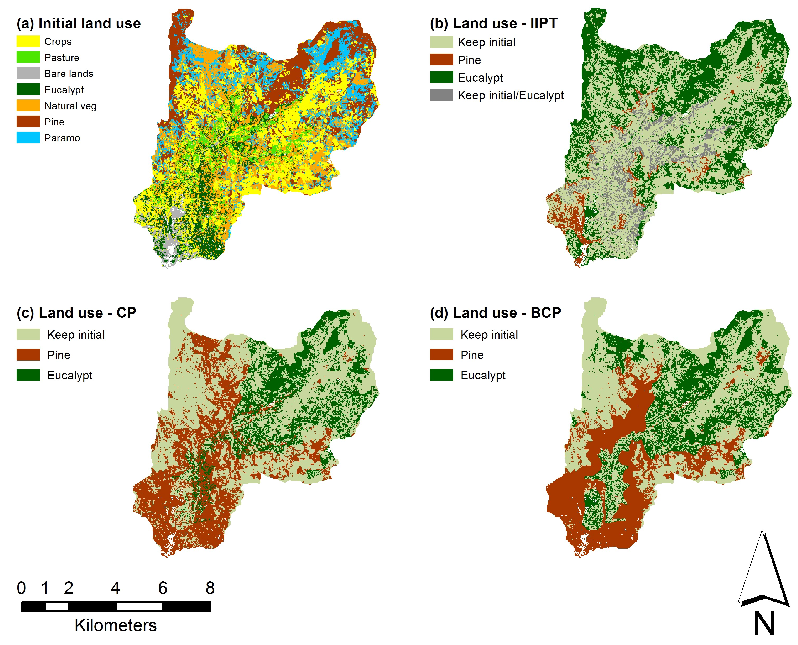
The land use type distribution suggested by each of the studied methods is shown in Figure 2. The initial land use map is included for reference.

Figure 2. (a) Initial land use map; LUT distribution resulting from: (b) IIPT; (c) CP; and (d) BCP.

Figure 2. (a) Initial land use map; LUT distribution resulting from: (b) IIPT; (c) CP; and (d) BCP.

When maps (b–d) are compared, it is noticeable that both CP-derived models favor the change to pine, while IIPT suggests to mostly keep land units under the iLUT or change them to eucalypt. It is especially remarkable that IIPT suggests to change most pine forests at higher altitudes to eucalypt. This may be an indication of the emphasis that the interval-based approach of IIPT puts on the criteria with higher relative importance (smaller intervals), as is the case for income in this study, since, according to the available data, eucalypt forests produce considerably larger profits than pine forests. In other words, IIPT focuses more on optimizing criteria with high weights at the expense of solution balance, even when compared to the canonical CP.

The LUT distributions proposed by CP and BCP are quite comparable for the particular combination of parameter values that was chosen. This similarity in the output was already revealed by the coincidence index. However, when more emphasis is given to solution balance, by increasing the λ parameter, it is expected that the difference between the output of CP and BCP increases.

4. Discussion and Conclusions

Two established MCDM, namely IIPT and CP, and BCP as a novel one, were applied to a database representing the expected cumulative performance in terms of five ecosystem services of the 417 land units covering the Tabacay River catchment after 30 years of continuation of the initial land use type and 30 years after a land use change to pine or eucalypt forest. The goal was to design a LUT-configuration to be applied to the full study region in order to optimize integrated land performance.

These methods are all part of a family of MCDM that select alternatives based on their closeness to an “ideal point”, which corresponds to the optimal value of every criterion when evaluated independently of each other. IIPT was used to select the best performing LUT for every land unit separately from any other land unit. The LUT distributions generated by the CP-derived models, on the other hand, are targeted to the optimization of the integrated land performance of the full study region as a whole. The other difference between IIPT- and CP-based models is the way in which they search for optimal solutions. In the case of IIPT, thresholds are defined in such a way that separate deviations from the ideal value for each criterion are kept within restricted limits. In the CP-based models, on the other hand, deviations from the ideal point are normalized and then combined into a single distance function, which then becomes the objective function (to be minimized) of the resulting linear programming models. Additionally, the definition of these methods mean that CP and BCP can be applied to either discrete or continuous decision problems, while the IIPT requires that the set of decision alternatives is finite, i.e., it is only applicable to discrete problems.

A particular issue in IIPT, which can be seen as a drawback in some cases, is its incapability to distinguish among decision alternatives that present similar, although not identical, performance. Since IIPT uses an iterative procedure in which a threshold is defined and used at each step to filter alternatives with high performance, whenever more than one alternative meets a given threshold, a case of multi-alternative selection will occur. The presence of these cases in IIPT output complicates the interpretation of results and decreases the amount of information that can be distilled. Trends observed in the results indicate that IIPT is more targeted to achieve solutions that are most influenced by the criterion with the highest relative importance, which makes this method prone to producing unbalanced solutions, that is solutions that correspond to a near-to-optimal performance for the most important criterion and that perform poorly regarding the other criteria.

On the other hand, judging by the general similarity of the results produced by both CP-derived models, it can be concluded that they are suitable methods when a balanced solution is required. This fact is even more evident when considering the deviations from the ideal performance corresponding to the LUT distributions suggested by these methods. In particular, deviations for both methods is confined to similar levels, although this behavior is expected to change when more emphasis is allocated to solution balance in BCP. This expectation is not completely in line with, e.g., [27], who obtained virtually the same results with λ = 1 and with λ = 0 when applying CP to an environmental resources management problem, neglecting in practice the influence of the λ parameter on their model output. On the other hand, [28] found that both instances of CP (with λ = 0 and λ = 1) produced results differing within a limited range, which is much more comparable with the findings we made in our study. Note that, unlike BCP, the CP formulations of [27,28] do not allow values of λ different from zero and one. Clearly, discrepancies between applications of CP can be explained to a large extent by differences in the parameter settings, e.g., the relative importance assigned to criteria, and to the underlying database, in addition to the value set for the parameter λ.

For the parameter values used in our tests, CP and BCP performed in a similar way regarding solution balance, even though this aspect is not explicitly included in the CP model formulation. It is important to stress the importance of extending CP into BCP, since the explicit inclusion of solution balance considerations allows the user of this method a greater degree of flexibility, with the capability of emphasizing either solution balance or combined optimization achievement.

Regarding modularity, since the CP-derived methods rely on concepts of mathematical programming, they do not impose a great deal of effort to make specific adaptations to the model formulation. In particular, to integrate restrictions with respect to minimum and maximum areas for certain LUT or ESS-level thresholds to be met by the proposed land use type distribution, it would be sufficient to ideate and include the appropriate constraints in the model formulation. To introduce such adaptations in IIPT would undoubtedly require more effort, given its algorithmic nature and its lower level of modularity when compared to mathematical programming models.

Whereas in this study, only on-site ESS, like sediment production and carbon storage, were considered, a challenge is to also incorporate off-site ESS, like sediment transport and delivery [29], into the optimization of the land use distributions.

Another possibility for further elaboration of the presented methods is to accommodate temporal aspects either into the algorithm, in the case of IIPT, or into the model formulation, in the case of the CP-based models. The incorporation of time-related issues into the problem would require the availability of datasets corresponding to several points in time, so that answering questions like when to intervene in a territory or for how long to keep a given LUT becomes possible.

In-depth insights about the nature and functioning of these methods can be obtained from studying the impact that variations in the values of the different parameters have on the methods’ output. In particular, tests involving different parameter settings would provide a clearer idea about the solution space being dealt with. In this context, a sensitivity analysis involving the λ parameter in the case of the CP-based models and different weights values for all of the applied methods would shed some light on their behavior and internal working under different scenarios and would allow the user of the methods to determine more reasonable parameter values.

From our comparison of three ideal point-based multi-criteria decision methods, we recommend a regionally-integrated CP-based approach over the per-land unit IIPT approach to establish land use distributions that can serve as base maps for further operational land use planning. This suggestion does not imply that IIPT should be discarded without further consideration. IIPT can still be useful in other problem instances, as it has been shown in the past [9,10,11]. IIPT can be considered as a valid alternative, especially when the input data structure permits a clear differentiation among the values of individual criteria, since this characteristic will counteract the possibility of IIPT not being able to distinguish among several alternatives. Special care when setting criteria weights is also a requirement for using IIPT. As has been shown above, differences in weights have a large impact on the method outputs. Therefore, it is advised to avoid radical differences when expressing relative importance, especially in problem instances for which reasonable improvements for all criteria involved are required.