Article

Assessment of Low Density Full-Waveform Airborne Laser Scanning for Individual Tree Detection and Tree Species Classification

1
Finnish Geodetic Institute, Geodeetinrinne 2, Masala 02340, Finland
2
Department of Forest Sciences, University of Helsinki, P.O. Box 27, Helsinki FI-00014, Finland
*
Author to whom correspondence should be addressed.
Forests 2014, 5(5), 1011-1031; https://doi.org/10.3390/f5051011
Submission received: 7 March 2014 / Revised: 5 May 2014 / Accepted: 14 May 2014 / Published: 21 May 2014

Abstract

:
The paper investigated the possible gains in using low density (average 1 pulse/m2) full-waveform (FWF) airborne laser scanning (ALS) data for individual tree detection and tree species classification and compared the results to the ones obtained using discrete return laser scanning. The aim is to approach a low-cost, fully ALS-based operative forest inventory method that is capable of providing species-specific diameter distributions required for wood procurement. The point data derived from waveform data were used for individual tree detection (ITD). Features extracted from segmented tree objects were used in random forest classification by which both feature selection and classification were performed. Experiments were conducted with 5532 ground measured trees from 292 sample plots and using FWF data collected with Leica ALS60 scanner over a boreal forest, mainly consisting of pine, spruce and birch, in southern Finland. For the comparisons, system produced multi-echo discrete laser data (DSC) were also analyzed with the same procedures. The detection rate of individual trees was slightly higher using FWF point data than DSC point data. Overall detection accuracy, however, was similar because commission error was increased when omission error was decreasing. The best overall classification accuracy was 73.4% which contains an 11 percentage points increase when FWF features were included in the classification compared with DSC features alone. The results suggest that FWF ALS data contains more information about the structure and physical properties of the environment that can be used in tree species classification of pine, spruce and birch when comparing with DSC ALS data.

1. Introduction

The successful identification and characterization of individual trees is critical for precise forest mapping and modeling [1], particularly for more precise mapping of tree quality attributes, timber assortments [2], biomass and individual tree growth modeling [3,4,5,6]. Many modern systems for forest management planning also require forest information at the individual tree level [7,8,9].
Airborne Laser Scanning (ALS) is an active remote sensing technique which is capable of providing 3-Dimensional (3D) point clouds. It has been shown to be an efficient technique to characterize both forest structure [10,11,12,13,14,15,16,17], and ground topography [18,19,20,21]. In a growing number of countries, operational forest attribute inventory for forest management is based on ALS data, field plots and so-called area-based approach (ABA) [22]. ABA prediction of forest inventory attributes is based on the statistical dependency between the attributes measured in the field plots and the predictor features derived from ALS data. The sample unit in the ABA is most often a grid cell, the size of which corresponds to the field-measured training plots. Stand-level forest inventory results are aggregated by summing and weighting the grid-level predictions inside the stand. Non-parametric estimation is often favored to obtain all the required attributes simultaneously [22]. The increasing requirement of forest data users is towards species-specific diameter or volume distribution. The use of individual tree based ALS technology [23] is a potential solution for obtaining diameter and volume class distributions, but the species information is still needed.
Conventional laser scanner systems record multiple echoes from a single laser pulse. As the development of the technologies, full-waveform (FWF) scanners are capable of recording the complete echo signal. Multiple echoes are recorded in real time during the acquisition in the case of conventional systems whereas they are usually detected in a post-processing step in FWF systems by a FWF decomposition algorithm. Two types of laser scanners are available according to footprint: small-footprint and large-footprint systems. The former often acquires data from airborne platforms and the latter from satellite. Most FWF commercial systems are small-footprint (0.2–3 m diameter) and capture data from airborne platforms [24].
Previous studies have demonstrated the high information content of ALS FWF measurements and many methods have been developed to analyse the received waveform of the backscattered laser pulse in order to improve point extraction and/or obtain additional target information from the waveform shape [25,26,27]. For example, Persson et al [28] modeled FWF as a sum of Gaussian distributions. The estimated models were then used for extracting 3D points and other parameters associated with the distribution components. The number of additional points that were extracted ranged between 18% and 57% depending on the type of vegetation. In [25], Wagner et al. also used Gaussian distribution function to model the FWF. The fitted model parameters, i.e., amplitude, echo width, distance and cross-section, were then used for separating between vegetation and terrain, vegetation and non-vegetation. Thus, FWF data provide not only additional points but also additional information about reflecting objects compared to the conventional multi-echo ALS data. In addition, FWF-derived features have been demonstrated to be useful in tree species classification [29,30,31], for segmenting ALS point clouds in city areas [32] and in estimation of 3D vegetation structure [28,33]. A detailed state-of-the-art on FWF laser scanning can be found in [24].
A common practice for individual tree detection (ITD) is to combine tree top finding and crown delineating. Normally, the local maximum techniques are used to locate tree tops and then segmentation techniques are used for crown delineation. Morsdorf et al. [34] demonstrated an ITD method using cluster analysis. Reitberger et al. [35] used the combination of the stem detection method and normalized cut segmentation in 3D has led to the improvement in segmentation results. Moreover, the experiments showed clearly that using FWF data is superior to using first/last pulse data.
Following the tree delineation, a tree species classification is in most applications required. Several researchers have proposed methods of using multi-return discrete (DSC) ALS data for tree species classification [36,37,38,39]. Holmgren et al. [36] demonstrated an accuracy of 95% when classifying Scots pine and Norway spruce with the high density DSC data. In Brandtberg [37], a digraph process was used for tree species classification of leaf-off deciduous (oaks, red maple, and yellow poplar) based on DSC data (12 first returns/m2). The maximum total classification accuracy of 64% was achieved. Ørka et al. [38] reported an accuracy of 73% when classifying conifers and deciduous trees solely based on intensity measurements of DSC data (6.6 points/m2 in average). Kim et al. [39] showed that coniferous and the deciduous trees can be classified with an accuracy of 83.4% for the leaf-off state and 73.1% for the leaf-on state. Combining both leaf-on and leaf-off datasets they reached an accuracy of 90.6%. The leaf-off data have a point density up to 20 points/m2 and the leaf-on data up to 5 points/m2.
Most of the studies using DSC data for tree species classification were restricted to two or three species or species groups. To increase the probability for differentiating more species and/or improve the accuracy, features derived from FWF data have been used alone or in combination with features derived from DSC data. Vaughn et al. [40] reported an accuracy of 79.2% when classifying five species based solely on DSC data. Incorporating waveform information improved the overall accuracy to 85.4% using the FWF data of approximately 10 pulses/m2. Reitberger et al. [30] studied the use of intensity and pulse width for discriminating conifer and deciduous trees. With two data sets, both leaf-on and leaf-off conditions, they reached classification accuracies of 85% and 95%, respectively and mean pulse width of single reflections within a beam revealed to be the strongest discriminator. Höfle et al. [41] investigated mean echo width and backscatter cross section derived from FWF data to separate larch from deciduous trees using the FWF data of 16 points/m2 in average. Hollaus et al. [42] performed tree species classification in mixed woodland area using echo width, backscatter cross section, as well as the distribution of the echoes in vertical direction. The achieved overall accuracy was 83% based on a dataset of density ranging from 2–50 points/m2. Furthermore, the standard deviation of the echo widths per crown segment was proven useful for a separation of spruce and larch. Heinzel and Koch [43] explored a large suite of features including various intensity-related features for tree species classification with FWF data of 16 points/m2 and achieved an accuracy of 57% for six classes and 91% for two (conifers and broadleaved trees).
In practical forestry, costs of the inventory have to be minimized thus no one wants to pay for higher costs of ALS data acquisitions or several data sets. Therefore, the most desired solution for practical forestry is to use only slightly higher point density (e.g. 2 points/m2) that is already used to enable individual tree techniques. On the other hand, it would be beneficial if the tree species classification could be performed with ALS data and there would not be need for optical images that are often acquired to improve estimation of tree-species specific attributes.
Most of the research on FWF analysis was based on high density data due to the ability of such data to derive individual tree structure. With such data, both good-quality individual tree recognition and tree species classification can be performed [30,41,42,43]. On the other hand, in an international comparison study [44], it was found that the impact of point density of ALS data on ITD was marginal when 2, 4 and 8 points/m2 datasets were compared in boreal forest conditions. Thus, the use of a low density FWF data could be beneficial due to possible improvement in tree species classification and only a slight increase in costs. Therefore, the current study presents approaches to detect individual trees from relatively low density (1 pulse/m2) FWF ALS data, and to classify tree species and explore the most significant features for tree species classification using random forest technique [45]. The analyses are performed with the aim to investigate whether the low density small footprint waveform data performs better than conventional multi-echo data obtained simultaneously in individual tree detection and tree species classification.

2. Study Area and Material
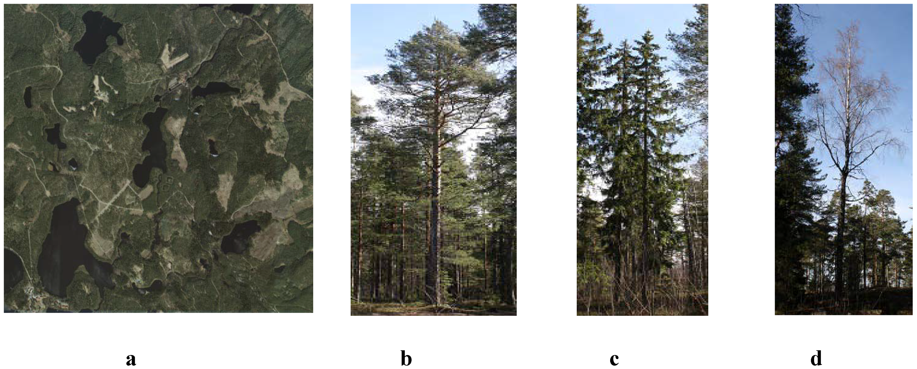
2.1. Study Area

The study area is located in Evo, southern Finland (61.19° N, 25.11° E). The 5 km × 5 km test area is part of the southern Boreal Forest Zone. It contains approximately 2000 ha of managed boreal forest, having an average stand size of slightly less than 1 ha. The elevation of the area varies from 125–185 m above sea level. Scots pine (Pinus sylvestris) and Norway spruce (Picea abies) are the dominant tree species in the area, and they contribute 40% and 35% of the total volume, respectively, whereas the share of deciduous trees, mainly birch (Betula sp.), is 24% of the total volume. Therefore, we concentrated our study on classification of these three tree species. Figure 1a shows a section of an orthophoto taken from the study area. Figure 1b–d shows a ground photo of each of three major tree species.
Figure 1. Test site photos: (a) a section of orthophoto; (b) a pine; (c) a spruce and (d) a birch; photos were taken at the different date than ALS (Airborne Laser Scanning) acquisition.
Forests 05 01011 g001

2.2. Field Measurements

Field measurements were undertaken in summer 2009 on 292 circular plots (10-m fixed radius). Sampling of the field plots was based on pre-stratification of existing stand inventory data. The plots were selected so that they would represent different forest densities, ages, site types and tree species. The center of the plots was measured with a global positioning system (GPS) device and the locations were post-processed with local base station data. The resulting accuracy was expected to be 1–5 m. The positions of the trees were determined using the direction and distance of trees relative to the plot centre with an accuracy of 10–20 cm. Therefore, tree positions have a high precision, but low accuracy. In order to remove the bias in the measurements of the tree positions, each sample plot was visually examined against ALS data and possible errors in the measurements of plot center were corrected. Within the field plot, all trees with a diameter at breast height (DBH) of over 5 cm were tallied and tree species was recorded. Tree height was measured using Vertex clinometers and DBH with steel calipers. The descriptive statistics of the trees are summarized in Table 1.
Table 1. Summary of the field measurements data for the 292 sample plots (5532 trees) located in the study area.
Tree speciesMin.Max.MeanStandard deviationNumber of trees
Tree height (m)Pine4.335.216.85.72613
Spruce4.234.218.67.11726
Deciduous3.633.015.45.71193
DBH (cm)Pine7.063.118.17.8
Spruce7.069.816.08.7
Deciduous7.059.513.56.8
Plot density (trees/ha) 31.82037.2603.0388.6

2.3. ALS Data

Laser scanning data were collected in July 2010 when trees were in leaf-on conditions, using a Leica ALS60 system operating at a pulse rate of 117 kHz and a wavelength of 1064 nm. The system enables both FWF and DSC data collections that operates in parallel. The data were acquired at a flight altitude of 2000 m above ground level, resulting in an average density of 1 pulse/m2 in non-overlapping areas and a footprint size of 44 cm in diameter. The system digitally sampled and stored the entire echo waveform of the reflected laser pulse at a sample interval of 2 ns resulting in maximum 128 samples. This is equivalent to a discrete vertical section of 38.4 m. Up to four returns were recorded for DSC data. A total area of 9 km2 was covered with a scan angle of a total 30 degrees by 11 parallel flight tracks, which had a width of approximately 1100 m and an overlap of 50%. When plots are covered by more than one flight, data from the flight with a smaller scan angle were used in the analyses.

3. Methods

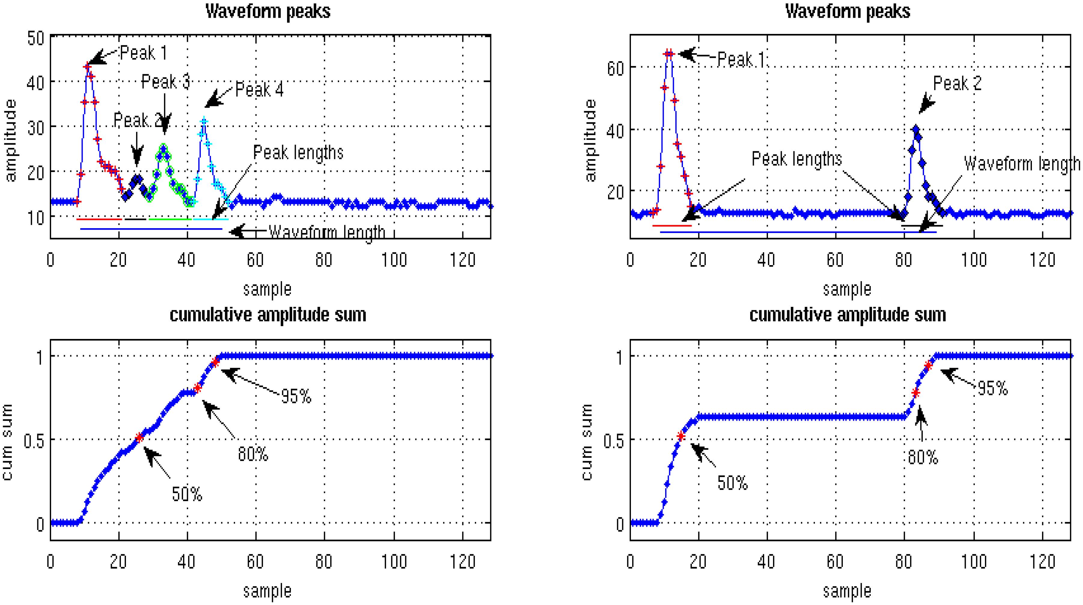
3.1. Full Waveform Decomposition and Features

The received waveform is generally decomposed by fitting Gaussians to the waveform [30,33]. In this study, we use a simple algorithm to detect peaks and retrieve the FWF features. The waveform is basically a list of amplitudes taken in small time intervals. These amplitudes are called samples in the following. The first and last parts of the waveform recordings were used to determine a common noise level to be used for all waveform recordings in this data. We used the difference (discrete derivative) between samples above noise level to mark the different peaks. When the signal amplitude drops below noise level, the value of the discrete derivative is greater than one. To avoid noise induced small peaks, a minimum length was set and all peaks with smaller length were discarded. To find peaks that were not separated by a drop to the noise level, the above noise parts were cut into peaks by taking the sign of the discrete derivative and following the rise (positive difference) to descent (negative difference), the start of a new rise started a new peak. The peaks and their amplitudes for two waveforms are plotted in the top row of Figure 2. Position of the detected peak echoes were calculated based on the range at maximum for each peak. The position of the waveform points is thus slightly different from the DSC points, because the trigger rule is different.
In addition to these extracted points from waveform data, the following FWF features were also computed.
  • N: Number of peaks extracted from the waveform;
  • E: Sum of the waveform samples above the noise level;
  • A_i: peak amplitude for the first four returns (peaks), i = 1, 2, 3, 4;
  • W_i: number of samples that constitute the peak for the first four returns (peaks), i = 1, 2, 3, 4;
  • R: waveform range calculated as the Euclidean distance between the first and the last peaks that was extracted from the waveform. This is shown as a blue line at the bottom of the top row waveform pictures in Figure 2;
  • DB_i: distance between first above noise point and the point at which 50%, 80% and 95% of the energy is received (cumulative sum of amplitudes), i = 50, 80, 95;
  • DA_i: Above ground height for 50%, 80% and 95% of the total waveform (cumulative sum of amplitudes), i = 50, 80, 95.
DB_i and DA_i features were used to describe the distribution of the total received energy which was estimated by computing the cumulative sum of the waveform and dividing with the total sum of the waveform (noise excluded in both). The bottom row of Figure 2 illustrates the cumulative amplitude sum for two waveforms.
Figure 2. Illustration of features computed from the waveforms; on the top row, the waveforms are divided into peaks; peak lengths are marked below the waveform with corresponding colors; the total waveform length is shown below the peak lengths; the minimum peak length is five samples; the noise threshold level used is 14; the cumulative amplitude sum is shown in the bottom row.
Forests 05 01011 g002

3.2. Individual Tree Detection

DSC data were first classified into ground or non-ground points using the standard approach of the TerraScan based on the method explained in [46]. A digital terrain model as a triangulated irregular network (TIN) was then created using classified ground points. The DSC points and FWF points were then normalized (normalized height or canopy height) by subtracting the ground elevations from both DSC points and FWF points at corresponding positions using DSC TIN model. Normalized points close to zero were considered as the returns from ground and those greater than 2 m from vegetation. The returns from vegetation were used for tree feature extraction.
A raster canopy height model (CHM) with a 0.5 m grid size was created from normalized data for all plots inside the coverage of ALS data for individual tree detection and crown segmentation. CHM was smoothed by applying a Gaussian filtering. Single-tree segmentations were then performed on smoothed CHM images using a minimum curvature-based region detector [47]. During the segmentation processes, the tree crown shape and location of individual trees were determined based on the segment outline and the location of maximum hit within the segment.
Detected trees were linked with the trees measured in the field by an automatic matching algorithm [48]. In the matching procedure, the distance between detected tree and the ground measured tree location was used as a matching criterion. If the ground-measured tree is the closest to one tree segments and vice versa and the distance between them is less than a threshold, then the tree is treated as correctly detected. Considering the possible difference in tree location measurements from ALS data (at tree top) and in the field (at tree root) and tree height underestimation by laser scanning, a 5 m threshold was used. The ground measured trees without any link to a tree segment are considered as non-detectable trees and a tree segment without a link to a reference tree results in a commission error.

3.3. ALS-Derived Features for Trees

For each detected tree, FWF data were extracted if it falls within the boundary of the detected tree and FWF descriptive statistical values (maximum, mean, and standard deviation) are derived from all FWF per tree segment for all FWF features, i.e., features described in Section 3.1. In addition, 27 DSC features were calculated from all normalized vegetation points of DSC data as some of them have been used in previous studies for individual tree attributes estimation [47]. Table 2 gives a list of the DSC and FWF features used in this study. FWF features were described in Section 3.1. Altogether, there are 78 features.
Table 2. DSC (Discrete) features calculated from all normalized vegetation points of DSC data and descriptive statistical values of full-waveform (FWF) features.
IndexFeatureDescription
DSC Features
1 PPulse penetration as the ratio of ground hit to total hits
2 mHArithmetic mean of heights
3 sHStandard deviation of heights
4 rHRange of height
5 CACrown area as the area of convex hull in 2D
6 CVCrown volume as the convex hull in 3D
7–16 H_i0th to 90th percentile of canopy height distribution with a interval of 10%
17 maxHHeight Maximum
18–26 DS_iPercentage of returns below 10%–90% of total height with a interval of 10%
27 MaxDMaximum crown diameter when crown was considered an ellipse
FWF Features
28–44 Mean (X)Average of all FWF hitting a tree for each feature described in Section 3.1, where X = {N, E, A_i, W_i, R, DB_i, DA_i}
45–61 Max (X)Maximum of all FWF hitting a tree for each feature described in Section 3.1, where X = {N, E, A_i, W_i, R, DB_i, DA_i}
62–78 Std (X)Standard deviation of all FWF hitting a tree for each feature described in Section 3.1, where X = {N, E, A_i, W_i, R, DB_i, DA_i}

3.4. Random Forest for Feature Selection and Classification

To classify tree species using the combination of DSC and FWF features, we are faced with a problem of high dimensional inputs (78 features). We need powerful algorithms for the classification and feature selection methods that can reduce input dimension.
Random forests (RF) technique is a type of ensemble classification that uses decision tree as the base classifier [45]. Given a set of class variables as responses and a list of potential features as predictors, the RF algorithm develops classifications by growing numerous decision trees. Each decision tree is constructed based on bootstrap samples selected randomly from a training dataset. The samples that are not used in the training are called “out-of-bag” (OOB) observations. RF computes the final class (prediction) by a majority vote over all constructed trees.
RF includes two important properties: random feature subspace and OOB estimates. The former enables a much faster construction of trees and the latter the possibility of evaluating the relative importance of each input feature [49]. One can use OOB data to estimate the feature importance by randomly permuting them across one feature at a time and estimating the increase in error due to this permutation; The larger the increase, the more important the feature. In addition, OOB estimates provide RF with a built-in cross-validation mechanism and therefore needs no separate validation dataset for evaluating the performance because the OOB data act in the same way as the validation dataset and give realistic prediction error estimates.
RF has been used in multisource and multivariate vegetation classification [50]. In Hudak et al. [51], RF technique was applied for imputing plot-level basal area and tree density for managed mixed-conifer forests in USA, using ALS data and compared with several other nonparametric regression methods. They concluded that the RF technique was the most robust and flexible method among those tested. Ørka et al. [38] used the RF method to classify tree species based on laser-derived features or a subset of features in Norway and compared the results with those of support vector machines (SVMs) and linear discriminant analysis (LDA). They obtained fairly similar accuracies, using all features and RF or SVM methods, compared with LDA and a feature-selection strategy.
Since a large number of laser features were tested, a trial and error procedure was used to identify the features which would contribute most in the classification. We started the iteration with all features and discarded the least important features in each trial until only 10 features remained. Classification accuracy was also calculated for each trial and analyzed. Fifteen features were selected because inclusion of more features did not increase the classification accuracy significantly. After determining the most important features, RF was run with 100 decision trees, four variables at each split of decision trees and 15 most important features selected for the tree species classification.

3.5. Accuracy Assessment

The accuracy of individual tree detection was evaluated by comparing the segmented trees with the reference trees measured in the field. Three measures were calculated as follows [1,52,53]:
Forests 05 01011 i001
Forests 05 01011 i002
Forests 05 01011 i003
where r is the tree detection rate, p is precision which indicates the correctness of the detected trees and F is F-score which gives an overall accuracy taking both commission and omission errors into consideration. Nt is the number of the detected trees which correctly linked with field-measured trees, No is the number of the trees which were not detected by laser data (omission error), Nc is the number of detected trees which do not exist in the field (commission error).
The accuracy of tree species classification was evaluated by comparing the classified tree species with the reference tree species recorded in the field. The result of the comparison can be represented by an error matrix. Three widely used measures, i.e., producer’s accuracy, user’s accuracy and overall accuracy, were computed for evaluating the performance of the classification. The producer’s accuracy refers to the probability that a certain tree species on the ground is classified as such, while the user’s accuracy refers to the probability that a segmented tree labeled as a certain species is really this class [54].

4. Results

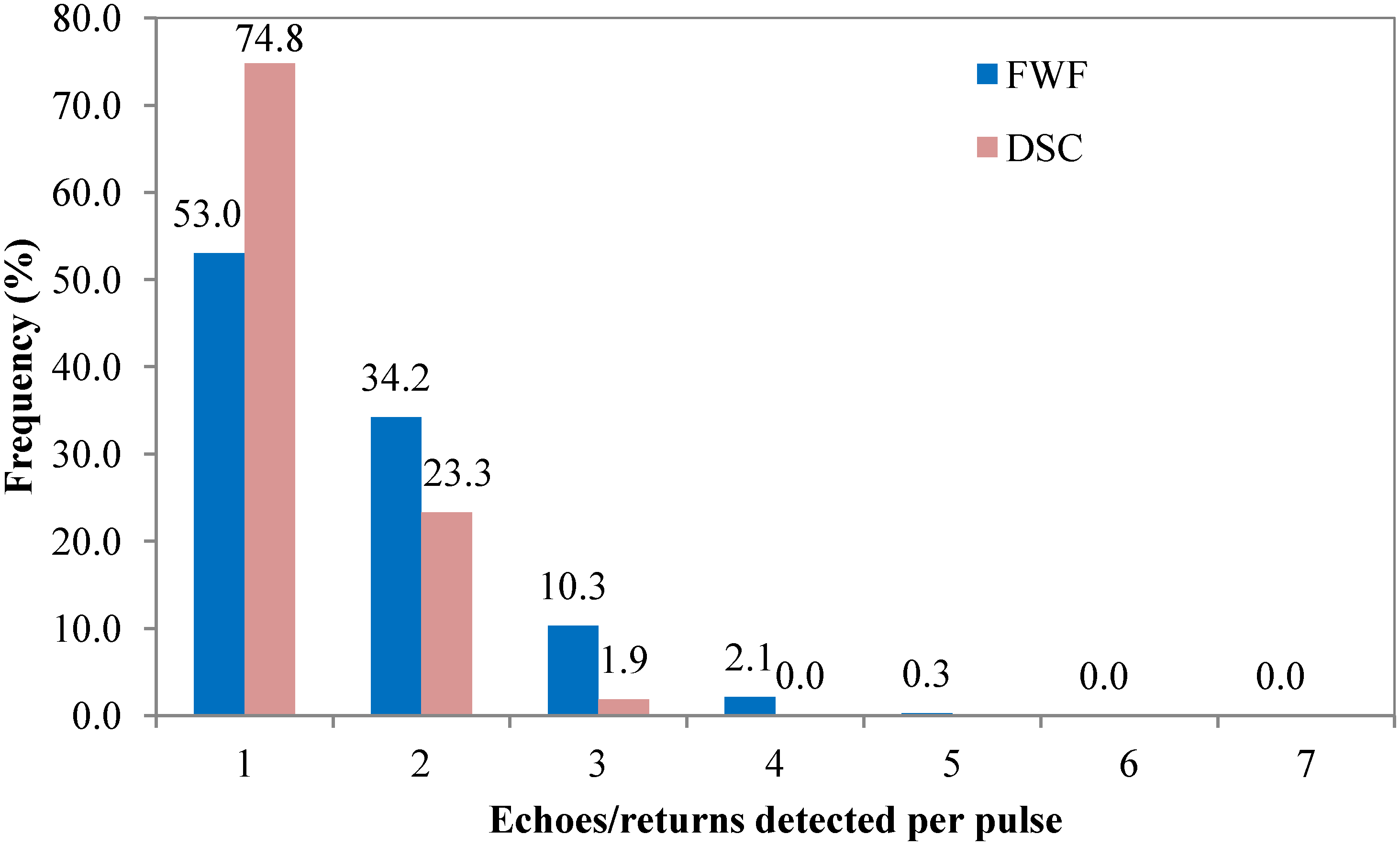
4.1. FWF(Full-Waveform) Decomposition

Up to seven echoes could be detected by FWF decomposition, while up to four returns were detected by the system. However, most of the pulses (over 95%) only produced up to three echoes from FWF data and up to two returns from the system (Figure 3). On average, DSC has a density of 1.5 points/m2 and FWF data a density of 2.4 points/m2. Figure 4 shows point clouds produced by the system and detected from FWF data for one sample plot.
Figure 3. Proportion of total detected echoes (returns) per pulse.
Forests 05 01011 g003
Figure 4. Point clouds produced by the system and detected from FWF in one sample plot; three hundred and ninety-one points recorded by the system and 639 points detected from FWF.
Forests 05 01011 g004

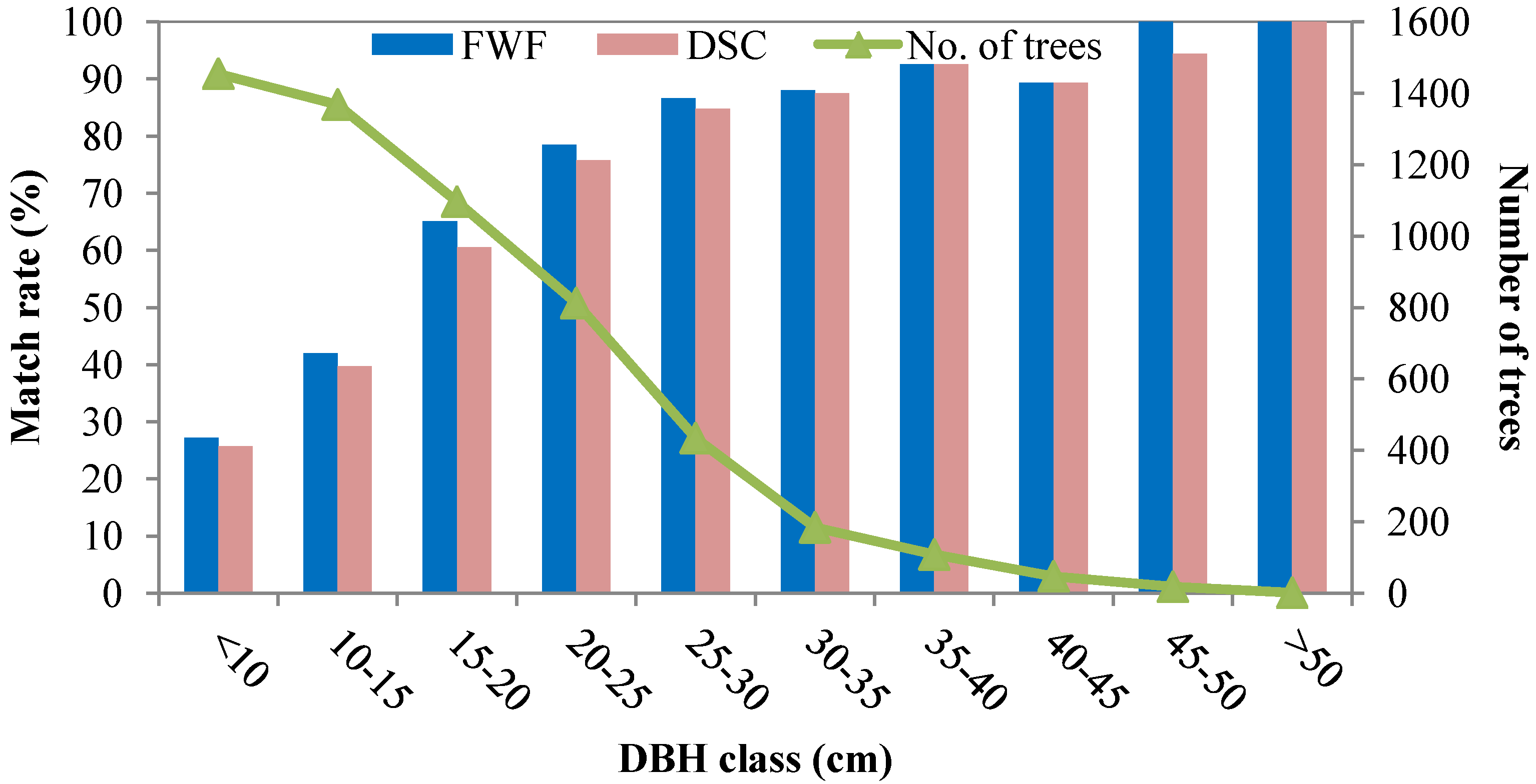
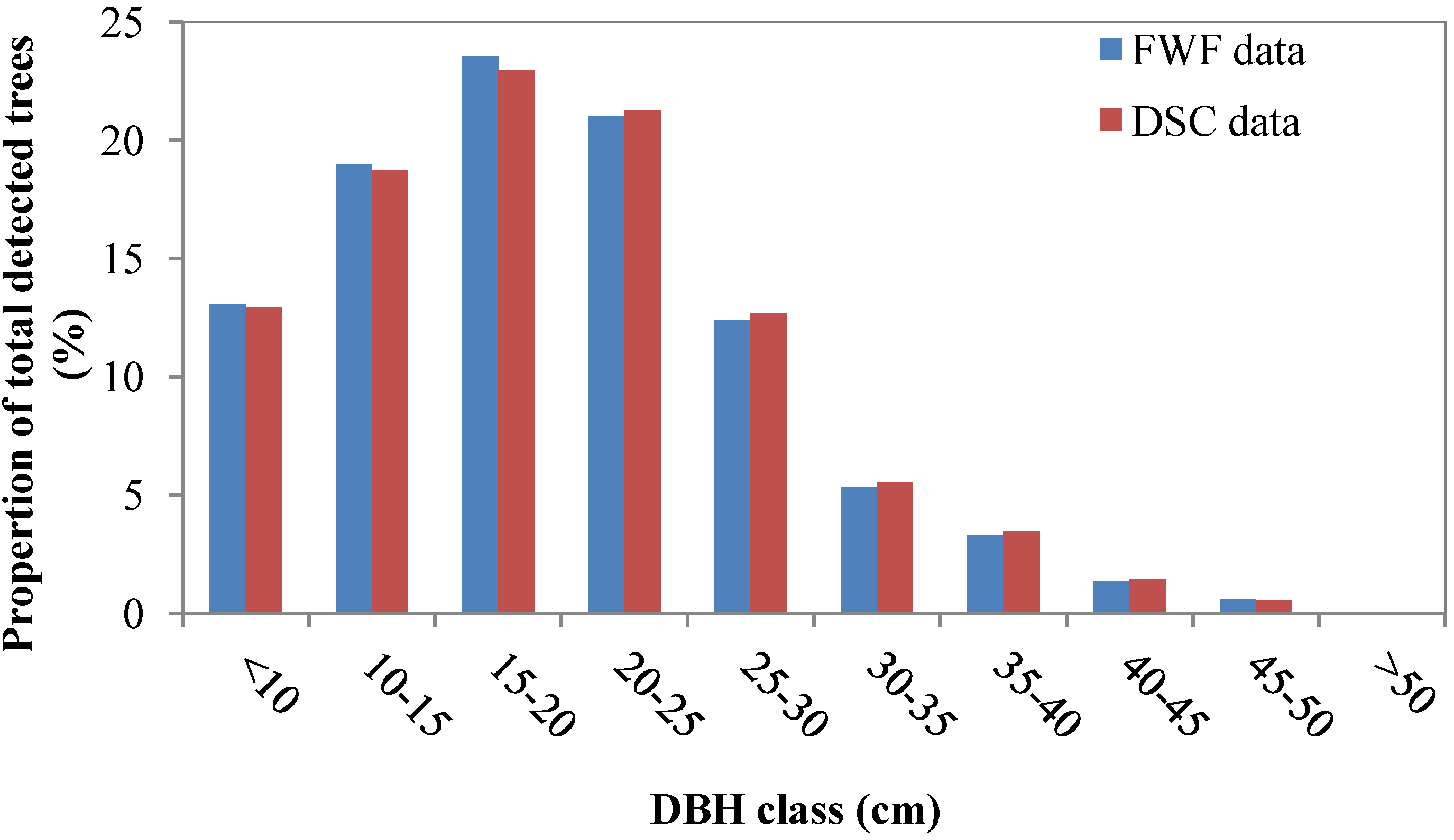
4.2. Individual Tree Detection

Individual trees were segmented separately from both FWF-derived point and DSC data as described in Section 3.2 for comparisons. The segmented trees were then compared with the reference trees in 292 plots. More trees were detected from FWF data (54.8% detection rate which corresponds 78% of the total stem volume) compared to DSC data (52.3% detection rate which corresponds 76% of the total stem volume). Figure 5 shows the individual tree detections as a function of DBH classes. As can be seen, trees not detected from the DSC data were detectable by the FWF point data, especially for smaller trees. DBH class distribution of mature trees is rather well represented by both FWF and DSC data (over 90% mature trees are correctly detected). This trend can also be illustrated by Figure 6 which shows the DBH distribution of detected trees from both data sets. However, the improvement is marginal as shown in Table 3 for the accuracy assessment of individual tree detection from both data sets. In Figure 7, detection rate is given by tree species.
Figure 5. Results of the individual tree detections: match rate as a function of DBH classes; the number of the trees in each diameter class is also shown in the figure.
Forests 05 01011 g005
Figure 6. The DBH distribution of correctly detected trees for DSC and FWF data sets.
Forests 05 01011 g006
Figure 7. Detection rate by tree species.
Forests 05 01011 g007
Table 3. Accuracy assessment for individual tree detection from DSC data and FWF data.
No. of detected treesNtNcNor (%)p (%)F (%)
DSC point data33622895467263752.386.165.1
FWF point data36953030665250254.882.065.7

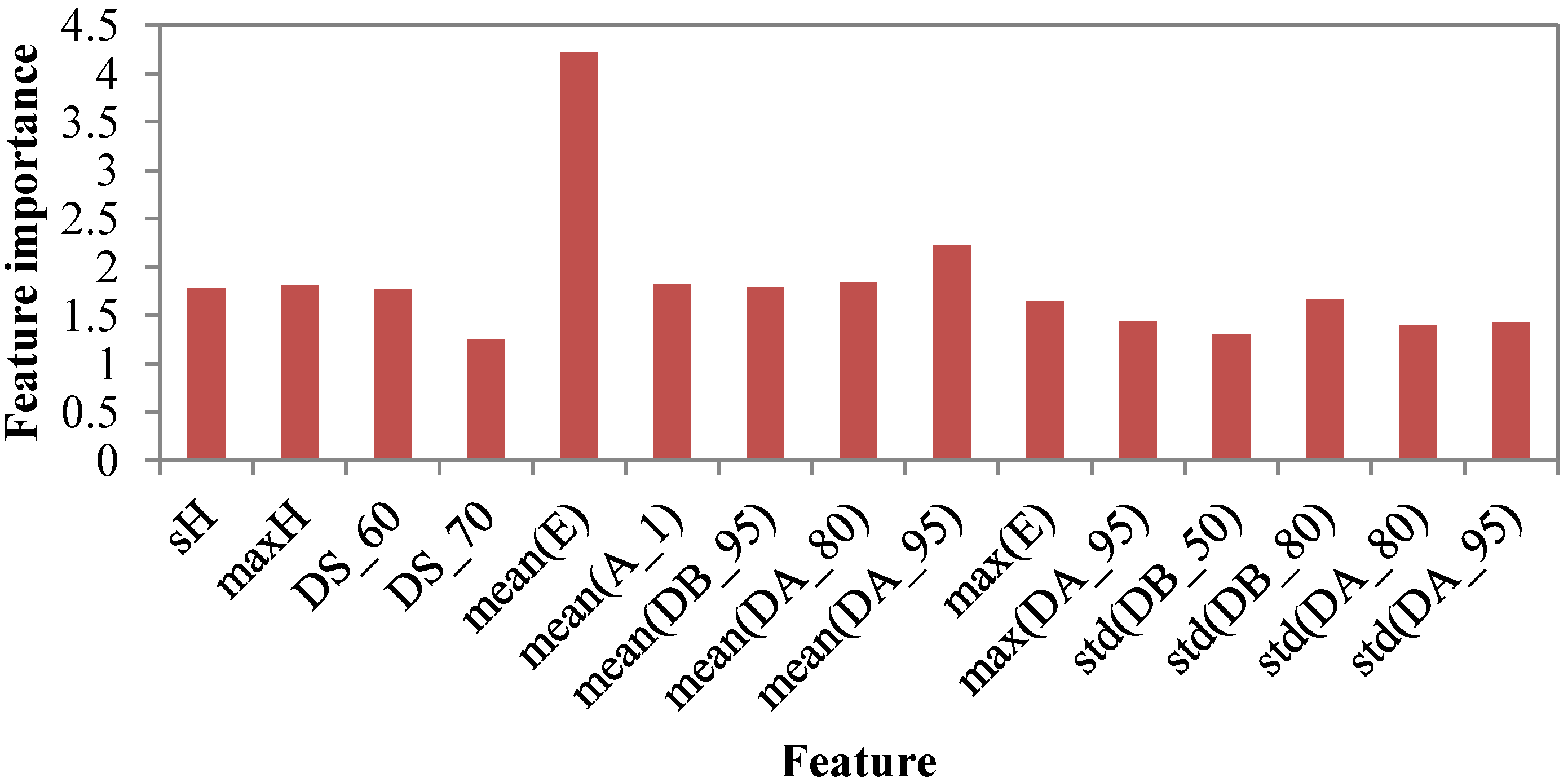
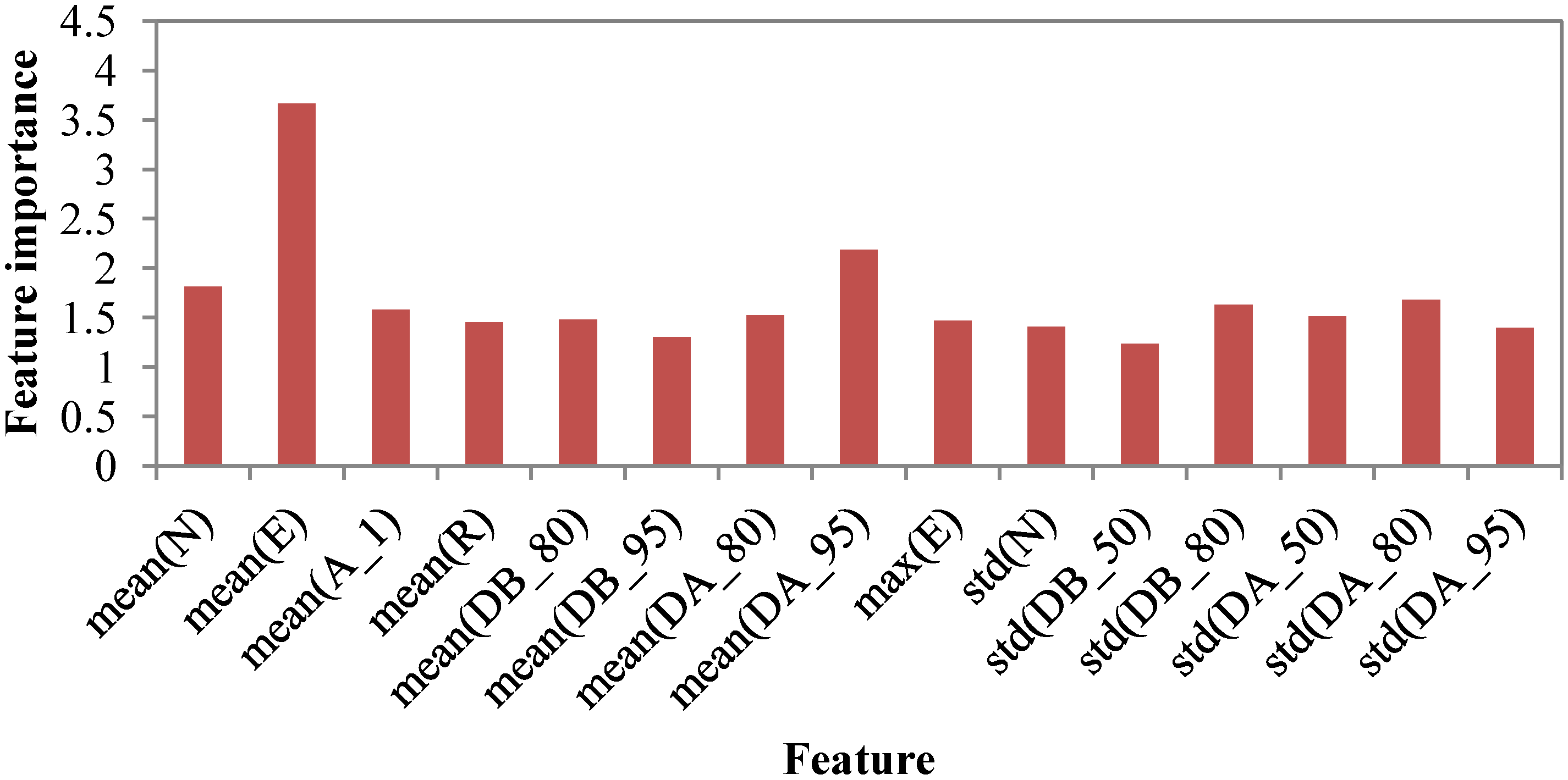
4.3. Feature Importance

Feature importance as a measure of prediction power is shown in Figure 8 where both DSC and FWF features were used as input in the tree species classification. Among 15 most significant features selected, four are DSC features (Figure 8, first four) and 11 are FWF features (Figure 8, last 11). As a comparison, 15 most significant features among FWF features and their importance are presented in Figure 9.
Figure 8. Feature importance for 15 most significant features selected from both DSC and FWF features; the greater the value, the more important the feature.
Forests 05 01011 g008
Figure 9. Feature importance for 15 most significant features selected from FWF features; the greater the value, the more important the feature.
Forests 05 01011 g009

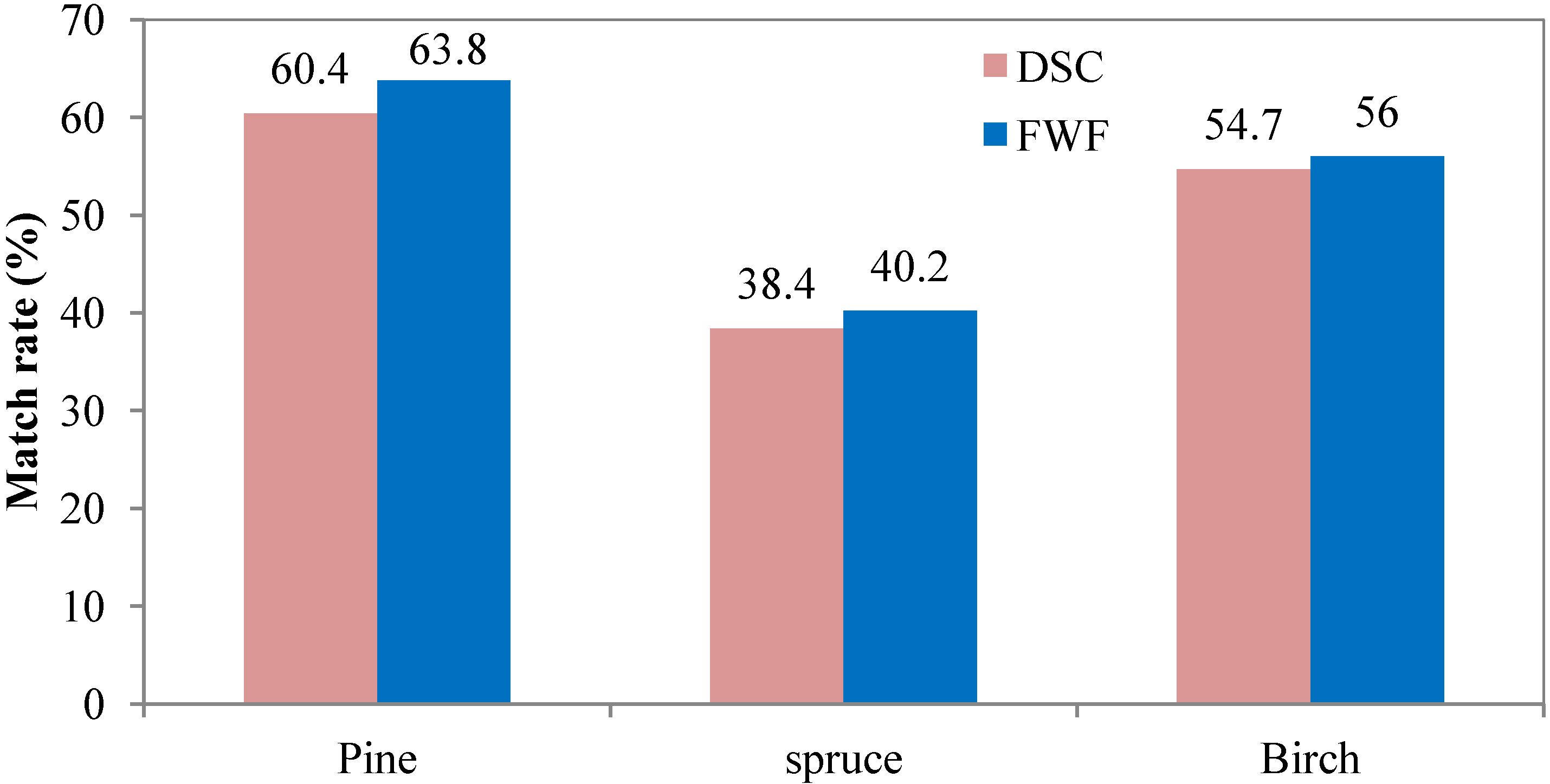
4.4. Tree Species Classification

Tree species classification was performed only for correctly detected trees based on DSC and FWF features combined as well as DSC features alone to investigate how FWF features improved the classification accuracy.
Classifications were performed based on 15 selected features for both cases and error matrix between reference and predicted classes is given in Table 4. Table 5 shows accuracy assessment by three measures for the classifications. It can be seen that all the accuracies were improved with varying degree for different species when FWF features were included in the classification. The overall accuracy was 62.1% with DSC features alone and 73.4% with both DSC and FWF features. The producer’s accuracies were improved by 5–30 percentage points and the user’s accuracy by 8–23 percentage points. For individual species, 81.3% of pine, 47.1% of spruce and 30.8% of birch were correctly classified with DSC data. Incorporating the FWF features improved accuracy from 81.3% to 86.2% for pine, from 47.1% to 55.4% for spruce and from 30.8% to 60.5% for birch. The biggest improvement was for birch (nearly 30 percentage points).
Table 4. Error matrix for the classifications using two sets of features.
Predicted class
With DSC featuresWith DSC and FWF features
PineSpruceBirchPineSpruceBirch
Reference classPine1284139156136212295
Spruce235312116186367110
Birch33911320116890395
Table 5. Three accuracy measures for the classifications using DSC features and together with FWF features.
With DSC FeaturesWith DSC and FWF features
Producer’s accuracyUser’s accuracyOverall accuracyProducer’s accuracyUser’s accuracyOverall accuracy
Pine81.369.1 86.379.4
Spruce47.155.3 55.463.4
Birch30.842.5 60.565.8
62.1 73.4
As a comparison, tree species classification was also carried out based on solely 15 most significant FWF features. The error matrix and accuracy measures of the classification are presented in Table 6. Overall classification accuracy is decreased from 73.4% to 71.5% using solely FWF features compared with FWF and DSC features combined (Table 5). However, accuracy of 71.5% is much higher than 62.1% accuracy when solely DSC features were used in the classification.
Table 6. Error matrix and accuracy of the classification with solely FWF features.
Predicted class
PineSpruceBirchProducer’s accuracy (%)
Reference classPine135612310085.9
Spruce21733710950.8
Birch1859137757.7
User’s accuracy (%) 77.161.264.3overall = 71.5

5. Discussion

5.1. Individual Tree Detection

In comparison to the use of DSC points, overall improvement for individual tree detection using FWF derived points are found to be marginal (from 52.3% to 54.8%) although FWF data is capable of detecting more smaller trees. There are several factors that can contribute to this. Firstly, Kaartinen et al. [55] found that detection method was a major factor of influencing the tree detection results. The marginal improvement in ITD could partially contribute to the method used which is based on CHM. Normally, CHM is created by taking the highest point value within a given area and the rest of the points in the area are ignored. Thus, the ability of producing more returns from FWF data is not fully utilized. In order to take full advantage of FWF data we recommend using the techniques based on point cloud clustering when FWF data is involved for ITD.
Secondly, leaf-on condition of trees during the laser data acquisition also prevented laser pulse from penetrating the canopy layers of deciduous trees. In closed canopy forests, there is also a significant reduction in the number of laser pulses that reach the forest understory. Reitberger et al. [35] demonstrated that a higher detection rate for the leaf-off data set mainly in the lower and intermediate layers because of the higher penetration of the deciduous trees in the leaf-off situation and higher density data.
Finally, the low density of laser data is another factor which may contribute the relatively low detection rate. Normally, data with the density of more than 5 points/m2 have been used for ITD to achieve an acceptable degree of accuracy [34,35]. In this study, data with an average of 1 pulse/m2 were used, thus lower detection accuracy was expected. However, the obtained detection rates are comparable to the results obtained with denser ALS data [56,57] and thus the use of low-density FWF could be beneficial for forest industry to get more detailed size information of the standing trees if detection rate can be improved as for example in [35] where a robust 3D clustering algorithm is used for ITD.

5.2. Tree Species Classification

Classification accuracy was improved in this study for all tree species with the use of full waveform data. The producer’s accuracy of the birch is poor, which is only 30%, using DSC features alone in the classification. The reason for the low accuracy of this class with DSC data is probably related to the difficulties in accurate delineation of birch because of more complex crown shape and structure. ITD algorithm used tends to split large deciduous trees into multiple crown parts which results in one segment for each part. However, the classification accuracy is much higher (60.5%) when FWF were also used in the classification. This indicated that the vertical distribution of the FWF information yields specific characteristics for each tree species.
Errors in the classification can also be attributed to the data being acquired on leaf-on conditions. As previously noted, percent canopy cover strongly affects returns due to fractional interception of energy by scattered foliage within the laser footprint. Dense canopy (both conifer and deciduous trees) where the laser beam is fully intercepted in the crown will cause a low number of echo returns compared to leaf-off condition where otherwise will produce more intermediate returns which provide more information on the vertical structure of the trees.
Classification accuracy is not balanced between the tree species. Pine trees were classified with a relatively high accuracy. There is, however, a relatively high degree of confusion between pine and birch and between pine and spruce, i.e., the trend existed that more birch and spruce were misclassified as pine, regardless which feature group was used, resulting in a relatively low accuracy for spruce and birch. The higher classification accuracy for pine is probably due to the larger number of samples distributed across diverse stands.
In terms of feature importance, It can be seen that segment-based mean values have more predictive power than segment-based maximum and standard deviation values. Among the segment-based mean value, the sum of waveform samples are the most powerful features to separate the tree species, followed by above ground height of 95% FWF energy indicating that the structure difference between tree species contributed greatly to the reflectance difference. Regarding DSC features, standard deviation of the height, maximum height and canopy cover percentile at 60% of the tree height have almost equal power for classifying pine, spruce and birch. These DSC features can be replaced by FWF features without scarifying much classification accuracy (Table 6). We found that overall classification accuracy based on FWF features alone is slightly decreased compared with the accuracy based on both FWF and DSC features. In this case, four selected DSC features are replaced by mean and standard deviation of the number of peaks and mean value of the waveform range (Figure 9). The rest of the significant FWF features turned out to be almost the same as in the classification of combining DSC and FWF features.
It should be noted that species classification results are representative for trees that were detectable in dominant and co-dominant crown layers because suppressed trees are difficult to detect by the segmentation methods based on CHM. Further investigations are needed for studying the impact of ITD on species classification.
It would be interesting to know how well the low density data used in this study worked compared to other studies whereby higher density data were used. However, it should be noted that direct comparison is not possible because the results are highly data and site dependent. The accuracy achieved in this study is promising given that the density of data is much lower than the data used in other studies. For example, in Heinzel and Koch [43], accuracy of 78% was achieved for four species (pinus, spruce, oak and beech) classification. In Hollaus et al, [42], an accuracy of 75% for three tree species (red beech, larch and spruce) was reached. In both studies, the density of the data is higher than the one used in this study (16 points/m2 in [43] and 2–5 points/m2 in [42]). Höfle et al. [58] investigated the effect of data densities on the classification of the city scene and found out that classification accuracy remained relatively stable for point densities higher than 5 points/m2 and with point densities lower than 5 points/m2 classification accuracy can drop dramatically.

6. Conclusions

In this study, we assess the utility of relatively low density FWF data for individual tree detection and species classification in mixed coniferous forests in boreal zone to meet the needs of future forest inventories: improvements to species-specific results. Data with an average of 1 pulse/m2 resulted in comparable accuracies that have been obtained with higher point densities, for example 5 pulses/m2, at individual tree level. It should be noted that detection rate of individual trees is relatively low (54.8% and 52.3%) in this study. Further improvements are possible for individual tree detection by using 3D segmentation techniques which can take advantage of more spatial points that the full waveform data provided.
The results suggest that additional FWF features may be a valuable source of information for tree species classification of pine, spruce and birch which are the main tree species in boreal forest zone. The best overall classification accuracy was 73.4%. Exploration of other waveform features such as intensity features is recommended for future research related to tree species classification.

Acknowledgments

The Academy of Finland is acknowledged for its financial support in the form of the projects “Science and Technology Towards Precision Forestry”, “Towards Improved Characterization of Map Objects”, “Interaction of LiDAR/Radar Beams with Forests Using Mini-UAV and Mobile Forest Tomography”, and “Centre of Excellence in Laser Scanning Research, www.fgi.fi/coelasr, decision 272195”.

Author Contributions

Xiaowei Yu carried out the research and wrote the first draft of the paper. Paula Litkey processed the full-waveform data. Markus Holopainen and Mikko Vastaranta were responsible for the field measurements. Juha Hyyppä provided the scientific guidance. All co-authors assisted with improving the manuscript.

Conflicts of Interest

The authors declare no conflict of interest.

References

  1. Li, W.; Guo, Q.; Jakubowski, M.K.; Kelly, M. A new method for segmenting individual trees from the LiDAR point cloud. Photogramm. Eng. Remote Sens. 2012, 78, 75–84. [Google Scholar] [CrossRef]
  2. Kankare, V.; Räty, M.; Yu, X.; Holopainen, M.; Vastaranta, M.; Kantola, T.; Hyyppä, J.; Hyyppä, H.; Alho, P.; Viitala, R. Single tree biomass modelling using airborne laser scanning. ISPRS J. Photogramm. Remote Sens. 2013, 85, 66–73. [Google Scholar] [CrossRef]
  3. Popescu, S.C.; Wynne, R.H.; Nelson, R.H. Measuring individual tree crown diameter with LiDAR and assessing its influence on estimating forest volume and biomass. Can. J. Remote Sens. 2003, 29, 564–577. [Google Scholar] [CrossRef]
  4. Yu, X.; Hyyppä, J.; Kaartinen, H.; Maltamo, M. Automatic detection of harvested trees and determination of forest growth using airborne laser scanning. Remote Sens. Environ. 2004, 90, 451–462. [Google Scholar] [CrossRef]
  5. Falkowski, M.; Hudak, A.; Crookston, N.; Gessler, P.; Smith, A. Landscape-scale parameterization of a tree-level forest growth model: A k-NN imputation approach incorporating LiDAR data. Can. J. For. Res. 2010, 40, 184–199. [Google Scholar] [CrossRef]
  6. Vepakomma, U.; St-Onge, B.; Kneeshaw, D. Response of a boreal forest to canopy gap openings: Assessing vertical and horizontal tree growth with multi-temporal LiDAR data. Ecolo. Appl. 2011, 21, 99–121. [Google Scholar] [CrossRef]
  7. Söderbergh, I.; Ledermann, T. Algorithms for simulating thinning and harvesting in five European individual-tree growth simulators: A review. Computers Electron. Agric. 2003, 39, 115–140. [Google Scholar] [CrossRef]
  8. Kärkkäinen, L.; Matala, J.; Härkönen, K.; Kellomäki, S.; Nuutinen, T. Potential recovery of industrial wood and energy wood raw material in different cutting and climate scenarios for Finland. Biomass Bioenergy 2008, 32, 934–943. [Google Scholar] [CrossRef]
  9. Lindberg, E.; Holmgren, J.; Olofsson, K.; Wallerman, J.; Olsson, H. Estimation of tree lists from airborne laser scanning by combining single-tree and area-based methods. Int. J. Remote Sens. 2010, 31, 1175–1192. [Google Scholar] [CrossRef]
  10. Næsset, E. Predicting forest stand characteristics with airborne scanning laser using a practical two-stage procedure and field data. Remote Sens. Environ. 2002, 80, 88–99. [Google Scholar] [CrossRef]
  11. Lim, K.; Treitz, P.; Wulder, M.; St-Onge, B.; Flood, M. LiDAR remote sensing of forest structure. Prog. Phys. Geogra. 2003, 27, 88–106. [Google Scholar] [CrossRef]
  12. Zimble, D.A.; Evans, D.L.; Carlson, G.C.; Parker, R.C.; Grado, S.C.; Gerard, P.D. Characterizing vertical forest structure using small-footprint airborne LiDAR. Remote Sens. Environ. 2003, 87, 171–182. [Google Scholar] [CrossRef]
  13. Coops, N.C.; Hilker, T.; Wulder, M.A.; St-Onge, B.; Newnham, G.; Siggins, A.; Trofymow, J.A. Estimating canopy structure of Douglas-fir forest stands from discrete-return LiDAR. Trees Struct. Funct. 2007, 21, 295–310. [Google Scholar] [CrossRef]
  14. Vastaranta, M.; Wulder, M.A.; White, J.; Pekkarinen, A.; Tuominen, S.; Ginzler, C.; Kankare, V.; Holopainen, M.; Hyyppä, J.; Hyyppä, H. Airborne laser scanning and digital stereo imagery measures of forest structure: Comparative results and implications to forest mapping and inventory update. Can. J. Remote Sens. 2013, 39, 382–395. [Google Scholar]
  15. White, J.C.; Wulder, M.A.; Vastaranta, M.; Coops, N.C.; Pitt, D.; Woods, M. The utility of image-based point clouds for forest inventory: A comparison with airborne laser scanning. Forests 2013, 3, 518–536. [Google Scholar]
  16. Wulder, M.A.; Coops, N.C.; Hudak, A.T.; Morsdorf, F.; Nelson, R.; Newnham, G.; Vastaranta, M. Status and prospects for LiDAR remote sensing of forested ecosystems. Can. J. Remote Sens. 2013, 39. [Google Scholar] [CrossRef]
  17. Jaskierniak, D.; Lane, P.N.J.; Robinson, A.; Lucieer, A. Extracting LiDAR indices to characterize multilayered forest structure using mixture distribution functions. Remote Sens. Environ. 2011, 115, 573–585. [Google Scholar] [CrossRef]
  18. Kraus, K.; Pfeifer, N. Determination of terrain models in wooded areas with airborne laser scanner data. ISPRS J. Photogramm. Remote Sens. 1998, 53, 193–203. [Google Scholar] [CrossRef]
  19. Lee, H.S.; Younan, N. DTM extraction of LiDAR returns via adaptive processing. IEEE Trans. Geosci. Remote Sens. 2003, 41, 2063–2069. [Google Scholar] [CrossRef]
  20. Chen, Q.; Gong, P.; Baldocchi, D.; Xie, G. Filtering airborne laser scanning data with morphological methods. Photogramm. Eng. Remote Sens. 2007, 73, 175–185. [Google Scholar] [CrossRef]
  21. Mongus, D.; Žalik, B. Parameter-free ground filtering of LiDAR data for automatic DTM generation. ISPRS J. Photogramm. Remote Sens. 2012, 67, 1–12. [Google Scholar] [CrossRef]
  22. White, J.C.; Wulder, M.A.; Varhola, A.; Vastaranta, M.; Coops, N.C.; Cook, B.D.; Pitt, D.; Woods, M. A Best Practices Guide for Generating Forest Inventory Attributes from Airborne Laser Scanning Data Using the Area-Based Approach; Information Report FI-X-10; Natural Resources Canada, Canadian Forest Service, Canadian Wood Fibre Centre, Pacific Forestry Centre: Victoria, BC, Canada, 2013; p. 50. [Google Scholar]
  23. Hyyppä, J. Method for Determination of Stand Attributes and a Computer Program to Perform the Method. U.S. Patent 6,792,684, 28 October 1999. [Google Scholar]
  24. Mallet, C.; Bretar, F. Full-waveform topographic LiDAR: State-of-the-art. ISPRS J. Photogramm. Remote Sens. 2009, 64, 1–16. [Google Scholar] [CrossRef]
  25. Wagner, W.; Hollaus, M.; Briese, C.; Ducic, V. 3D vegetation mapping using small-footprint full-waveform airborne laser scanners. Int. J. Remote Sens. 2008, 29, 1433–1452. [Google Scholar] [CrossRef]
  26. Chauve, A.; Vega, C.; Durrieu, S.; Bretar, F.; Allouis, T.; Deseilligny, M.P.; Puech, W. Advanced full-waveform LiDAR data echo detection: Assessing quality of derived terrain and tree height models in an alpine coniferous forest. Int. J. Remote Sens. 2009, 30, 5211–5228. [Google Scholar] [CrossRef]
  27. Roncat, A.; Wagner, W.; Melzer, T.; Ullrich, A. Echo detection and localization in full-waveform airborne laser scanner data using the averaged square difference function estimator. Photogramm. J. Finl. 2008, 21, 62–75. [Google Scholar]
  28. Persson, A.; Söderman, U.; Töpel, J.; Ahlberg, S. Visualization and analysis of full-waveform airborne laser scanner data. In International Archives of Photogrammetry, Remote Sensing and Spatial Information Sciences; Copernicus Publications: Enschede, The Netherlands, 2005; Volume 36, (Part 3/W19); pp. 103–108. [Google Scholar]
  29. Reitberger, J.; Krzystek, P.; Stilla, U. Analysis of full waveform LiDAR data for tree species classification. In International Archives of Photogrammetry, Remote Sensing and Spatial Information Sciences; Copernicus Publications: Bonn, Germany, 2006; Volume 36, (Part 3); pp. 228–233. [Google Scholar]
  30. Reitberger, J.; Krzystek, P.; Stilla, U. Analysis of full waveform LiDAR data for the classification of deciduous and coniferous trees. Int. J. Remote Sens. 2008, 29, 1407–1431. [Google Scholar] [CrossRef]
  31. Rutzinger, M.; Höfle, B.; Hollaus, M.; Pfeifer, N. Object-based point cloud analysis of full-waveform airborne laser scanning data for urban vegetation classification. Sensors 2008, 8, 4505–4528. [Google Scholar] [CrossRef]
  32. Melzer, T. Non-parametric segmentation of ALS point clouds using mean shift. J. Appl. Geod. 2007, 1, 159–170. [Google Scholar]
  33. Lindberg, E.; Olofsson, K.; Holmgren, J.; Olsson, H. Estimation of 3D vegetation structure from waveform and discrete return airborne laser scanning data. Remote Sens. Environ. 2012, 118, 151–161. [Google Scholar] [CrossRef]
  34. Morsdorf, F.; Meier, E.; Kötz, B.; Itten, K.I.; Bobbertin, M.; Allgöwer, B. LiDAR-based geometric reconstruction of boreal type forest stands at single tree level for forest and wildland fire management. Remote Sens. Environ. 2004, 92, 353–362. [Google Scholar] [CrossRef]
  35. Reitberger, J.; Schnörr, Cl.; Krzystek, P.; Stilla, U. 3D segmentation of single trees exploiting full waveform LiDAR data. ISPRS J. Photogramm. Remote Sens. 2009, 64, 561–574. [Google Scholar] [CrossRef]
  36. Holmgren, J.; Persson, A. Identifying species of individual trees using airborne laser scanner. Remote Sens. Environ. 2004, 90, 415–423. [Google Scholar] [CrossRef]
  37. Brandtberg, T. Classifying individual tree species under leaf-off and leaf-on conditions using airborne LiDAR. ISPRS J. Photogramm. Remote Sens. 2007, 61, 325–340. [Google Scholar] [CrossRef]
  38. Ørka, H.O.; Naesset, E.; Bollandsas, O.M. Classifying species of individual trees by intensity and structure features derived from airborne laser scanner data. Remote Sens. Environ. 2009, 113, 1163–1174. [Google Scholar] [CrossRef]
  39. Kim, S.; McGaughey, R.J.; Andersen, H.E.; Schreuder, G. Tree species differentiation using intensity data derived from leaf-on and leaf-off airborne laser scanner data. Remote Sens. Environ. 2009, 113, 1575–1586. [Google Scholar] [CrossRef]
  40. Vaughn, N.R.; Moskal, L.M.; Turnblom, E.C. Tree species detection accuracies using discrete point LiDAR and airborne waveform LiDAR. Remote Sens. 2012, 4, 377–403. [Google Scholar] [CrossRef]
  41. Höfle, B.; Hollaus, M.; Lehner, H.; Pfeifer, N.; Wagner, W. Area-based parameterization of forest structure using full-waveform airborne laser scanning data. In Proceedings of SilviLaser 2008 the 8th International Conference on LiDAR Applications in Forest Assessment and Inventory, Edinburgh, Scotland, UK, 17–19 September 2008; pp. 229–235.
  42. Hollaus, M.; Mücke, W.; Höfle, B.; Dorigo, W.; Pfeifer, N.; Wagner, W.; Bauerhansl, C.; Regner, B. Tree species classification based on full-waveform airborne laser scanning data. In Proceedings of SilviLaser 2009the 9th International Conference on LiDAR Applications for Assessing Forest Ecosystems, College Station, TX, USA, 14–16 October 2009; pp. 54–62.
  43. Heinzel, J.; Koch, B. Exploring full-waveform LiDAR parameters for tree species classification. Int. J. Appl. Earth Obs. Geoinf. 2011, 13, 152–160. [Google Scholar] [CrossRef]
  44. Kaartinen, H.; Hyyppä, J. EuroSDR/ISPRS Project Commission II, Tree Extraction, Final Report. EuroSDR. 2008. Available online: http://bono.hostireland.com/~eurosdr/publications/53.pdf (accessed on 10 November 2012).
  45. Breiman, L. Random forests. Mach. Learn. 2001, 45, 5–32. [Google Scholar] [CrossRef]
  46. Axelsson, P. DEM generation from laser scanner data using adaptive TIN models. In Proceedings of the XIXth ISPRS Congress Commission I–VII, Amsterdam, The Netherlands, 16–23 July 2000; pp. 110–117.
  47. Yu, X.; Hyyppä, J.; Holopainen, M.; Vastaranta, M.; Viitala, R. Predicting individual tree attributes from airborne laser point clouds based on random forest technique. ISPRS J. Photogramm. Remote Sens. 2011, 66, 28–37. [Google Scholar] [CrossRef]
  48. Yu, X.; Hyyppä, J.; Kukko, A.; Maltamo, M.; Kaartinen, H. Change detection techniques for canopy height growth measurements using airborne laser scanning data. Photogram. Eng. Remote Sens. 2006, 72, 1339–1348. [Google Scholar] [CrossRef]
  49. Chan, J.C.W.; Paelinckx, D. Evaluation of random forest and adaboost tree-based ensemble classification and spectral band selection for ecotope mapping using airborne hyperspectral imagery. Remote Sens. Environ. 2008, 112, 2999–3011. [Google Scholar] [CrossRef]
  50. Reese, H.; Nyström, M.; Nordkvist, K.; Olsson, H. Combining airborne laser scanning data and optical satellite data for classification of alpine vegetation. Int. J. Appl. Earth Obs. Geoinf. 2014, 27, 81–90. [Google Scholar] [CrossRef]
  51. Hudak, A.T.; Crookston, N.L.; Evans, J.S.; Hall, D.E.; Falkowski, M.J. Nearest neighbor imputation of species-level, plot-scale forest structure attributes from LiDAR data. Remote Sens. Environ. 2008, 112, 2232–2245. [Google Scholar] [CrossRef]
  52. Goutte, G.; Gaussier, E. A probabilistic interpretation of precision, recall and F-score, with implication for evaluation. Adv. Inf. Retr. 2005, 3408, 345–359. [Google Scholar] [CrossRef]
  53. Sokolova, M.; Japkowicz, N.; Szpakowicz, S. Beyond Accuracy, F-Score and ROC: A Family of Discriminant Measures for Performance Evaluation, AI 2006; Advances in Artificail Intelligence; Sattar, S., Kang, B.H., Eds.; Springer Berlin: Heidelberg, Germany, 2006; pp. 1015–1021. [Google Scholar]
  54. Congalton, R.G. A review of assessing the accuracy of classifications of remotely sensed data. Remote Sens. Environ. 1991, 37, 35–46. [Google Scholar] [CrossRef]
  55. Kaartinen, H.; Hyyppä, J.; Yu, X.; Vastaranta, M.; Hyyppä, H.; Kukko, A.; Holopainen, M.; Heipke, C.; Hirschmugl, M.; Morsdorf, F.; et al. An international comparison of individual tree detection and extraction using airborne laser scanning. Remote Sens. 2012, 4, 950–974. [Google Scholar] [CrossRef] [Green Version]
  56. Heinzel, J.N.; Weinacker, H.; Koch, B. Prior-knowledge-based single-tree extraction. Int. J. Remote Sens. 2011, 32, 4999–5020. [Google Scholar] [CrossRef]
  57. Falkowski, M.J.; Smith, A.M.S.; Gessler, P.E.; Hudak, A.T.; Vierling, L.A.; Evans, J.S. The influence of conifer forest canopy cover on the accuracy of two individual tree measurement algorithms using LiDAR data. Can. J. Remote Sens. 2008, 34, 338–350. [Google Scholar] [CrossRef]
  58. Höfle, B.; Hollaus, M.; Hagenauer, J. Urban vegetation detection using radiometrically calibrated smallfootprint full-waveform airborne LiDAR data. ISPRS J. Photogramm. Remote Sens. 2012, 67, 134–147. [Google Scholar] [CrossRef]

