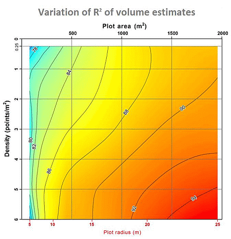
Analysis of the Influence of Plot Size and LiDAR Density on Forest Structure Attribute Estimates


Abstract
:
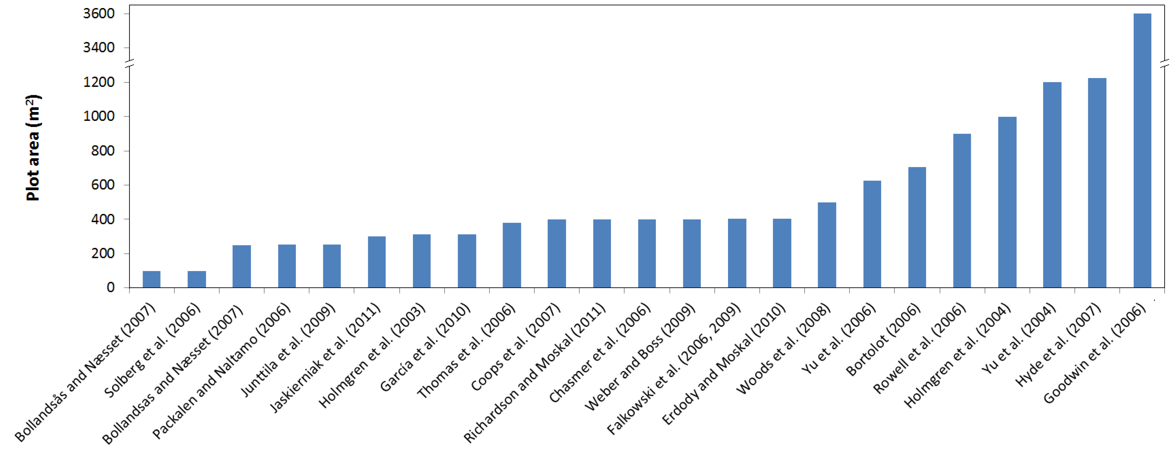
1. Introduction

2. Materials and Methods
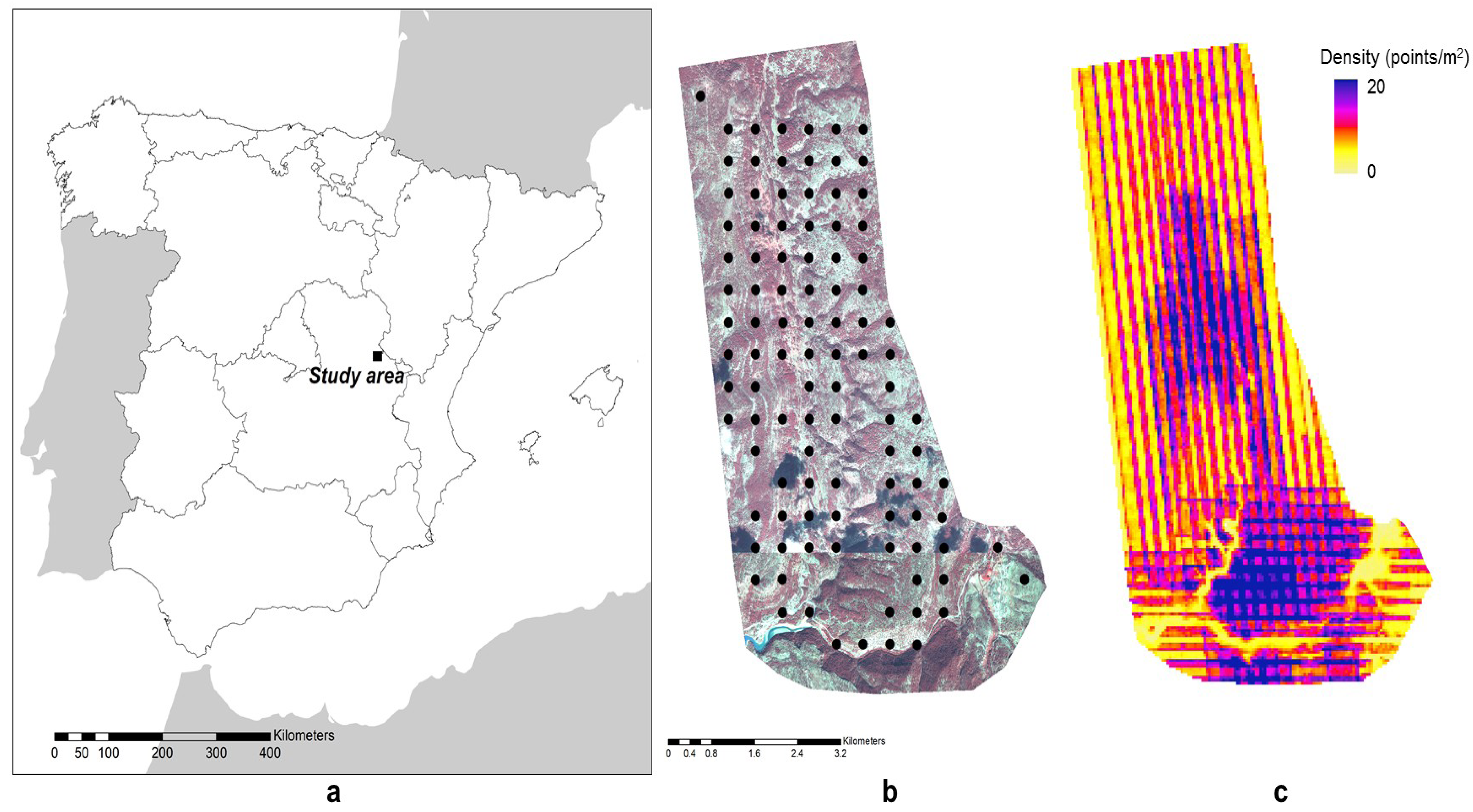
2.1. Study Area

2.2. Field Data

| Structure Attribute | Unit | Min. | Max. | Mean | Std Deviation |
|---|---|---|---|---|---|
| Volume | m3/ha | 0.13 | 271.70 | 65.80 | 49.61 |
| Total biomass | kg/ha | 274.9 | 167,518.7 | 50,010.7 | 30,299.9 |
| Basal area | m2/ha | 0.06 | 34.52 | 11.41 | 6.86 |
| Canopy cover | % | 0.14 | 63.86 | 25.55 | 12.80 |
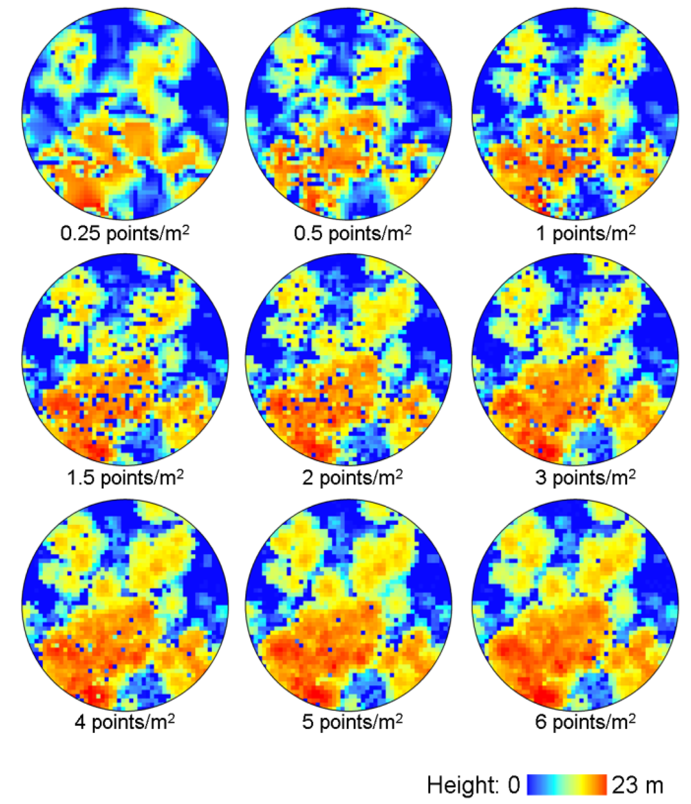
2.3. LiDAR Data
| Density (points/m2) | 0.25 | 0.5 | 1 | 1.5 | 2 | 3 | 4 | 5 | 6 |
| Number of plots | 102 | 102 | 102 | 102 | 100 | 98 | 91 | 58 | 50 |

2.4. Extraction of LiDAR Metrics and Model Generation for Forest Structure Estimates
| Symbol | Descriptive Feature |
|---|---|
| CHMμ | Average of the CHM height distribution |
| CHMσ | Standard deviation of the CHM height distribution |
| CHMRange | Range of the CHM height distribution |
| CHMKurtosis | Kurtosis of the CHM height distribution |
| CHMSkewness | Skewness of the CHM height distribution |
| CHMμedge | Average of the edgeness factor |
| CHMσedge | Standard deviation of the edgeness factor |
| Hμ | Average of the normalized point cloud height values |
| Hσ | Standard deviation of the normalized point cloud height values |
| HRange | Range of the normalized point cloud height values |
| HKurtosis | Kurtosis of the normalized point cloud height values |
| HSkewness | Skewness of the normalized point cloud height values |
| HP25 | 25th percentile of the normalized point cloud height values |
| HP50 | 50th percentile of the normalized point cloud height values |
| HP75 | 75th percentile of the normalized point cloud height values |
| HP100 | 100th percentile of the normalized point cloud height values |
| DPGP | Percentage of ground points in the density profile |
| DP1H | Height of the first peak of the density profile |
| DP1P | Percentage of points at the first peak of the density profile |
| DP2H | Height of the second peak of the density profile |
| DP2P | Percentage of points at the second peak of the density profile |
3. Results and Discussion


4. Conclusions
Acknowledgments
Author Contributions
Conflicts of Interest
References
- Mäkelä, H.; Pekkarinen, A. Estimation of forest stand volumes by Landsat TM imagery and stand-level field-inventory data. For. Ecol. Manag. 2004, 196, 245–255. [Google Scholar] [CrossRef]
- McRoberts, R.E.; Tomppo, E.O. Remote sensing support for national forest inventories. Remote Sens. Environ. 2007, 110, 412–419. [Google Scholar] [CrossRef]
- Van Leeuwen, M.; Nieuwenhuis, M. Retrieval of forest structural parameters using LiDAR remote sensing. Eur. J. For. Res. 2010, 129, 749–770. [Google Scholar] [CrossRef]
- Hyyppä, J.; Yu, X.; Hyyppä, H.; Vastaranta, M.; Holopainen, M.; Kukko, A.; Kaartinen, H.; Jaakkola, A.; Vaaja, M.; Koskinen, J.; et al. Advances in forest inventory using airborne laser scanning. Remote Sens. 2012, 4, 1190–1207. [Google Scholar] [CrossRef]
- Junttila, V.; Kauranne, T.; Leppänen, V. Estimation of forest stand parameters from airborne laser scanning using calibrated plot databases. For. Sci. 2010, 56, 257–270. [Google Scholar]
- Lovell, J.L.; Jupp, D.L.B.; Newnham, G.J.; Coops, N.C.; Culvenor, D.S. Simulation study for finding optimal LiDAR acquisition parameters for forest height retrieval. For. Ecol. Manag. 2005, 214, 398–412. [Google Scholar] [CrossRef]
- Gobakken, T.; Naesset, E. Assessing effects of laser point density on biophysical stand properties derived from airborne laser scanner data in mature forest. Int. Arch. Photogramm. Remote Sens. Spat. Inf. Sci. 2007, 36, 150–155. [Google Scholar]
- Frazer, G.W.; Magnussen, S.; Wulder, M.A.; Niemann, K.O. Simulated impact of sample plot size and co-registration error on the accuracy and uncertainty of LiDAR-derived estimates of forest stand biomass. Remote Sens. Environ. 2011, 115, 636–649. [Google Scholar] [CrossRef]
- Bollandsås, O.M.; Næsset, E. Estimating percentile-based diameter distributions in uneven-sized Norway spruce stands using airborne laser scanner data. Scand. J. For. Res. 2007, 22, 33–47. [Google Scholar] [CrossRef]
- Solberg, S.; Næsset, E.; Hanssen, K.H.; Christiansen, E. Mapping defoliation during a severe insect attack on Scots pine using airborne laser scanning. Remote Sens. Environ. 2006, 102, 364–376. [Google Scholar] [CrossRef]
- Packalén, P.; Maltamo, M. Predicting the volume by tree species using airborne laser scanning and aerial photographs. For. Sci. 2006, 52, 611–622. [Google Scholar]
- Jaskierniak, D.; Lane, P.N.J.; Robinson, A.; Lucieer, A. Extracting LiDAR indices to characterise multilayered forest structure using mixture distribution functions. Remote Sens. Environ. 2011, 115, 573–585. [Google Scholar] [CrossRef]
- Holmgren, J.; Nilsson, M.; Olsson, H. Estimation of tree height and stem volume on plots using airborne laser scanning. For. Sci. 2003, 49, 419–428. [Google Scholar]
- García, M.; Riaño, D.; Chuvieco, E.; Danson, F.M. Estimating biomass carbon stocks for a Mediterranean forest in central Spain using LiDAR height and intensity data. Remote Sens. Environ. 2010, 114, 816–830. [Google Scholar] [CrossRef]
- Thomas, V.; Treitz, P.; McCaughey, J.H.; Morrison, I. Mapping stand-level forest biophysical variables for a mixedwood boreal forest using LIDAR: An examination of scanning density. Can. J. For. Res. 2006, 36, 34–47. [Google Scholar] [CrossRef]
- Coops, N.C.; Hilker, T.; Wulder, M.A.; St-Onge, B.; Newnham, G.; Siggins, A.; Trofymow, J.A.T. Estimating canopy structure of Douglas-fir stands from discrete-return LiDAR. Trees Struct. Funct. 2007, 21, 295–310. [Google Scholar] [CrossRef]
- Richardson, J.J.; Moskal, L.M. Strengths and limitations of assessing forest density and spatial configuration with aerial LiDAR. Remote Sens. Environ. 2011, 115, 2640–2651. [Google Scholar] [CrossRef]
- Chasmer, L.; Hopkinson, C.; Smith, B.; Treitz, P. Examining the influence of changing laser pulse repetition frequencies on conifer forest canopy returns. Photogramm. Eng. Remote Sens. 2006, 72, 1359–1367. [Google Scholar] [CrossRef]
- Weber, T.C.; Boss, D.E. Use of LiDAR and supplemental data to estimate forest maturity in Charles County, MD, USA. For. Ecol. Manag. 2009, 258, 2068–2075. [Google Scholar] [CrossRef]
- Falkowski, M.J.; Smith, A.M.S.; Hudak, A.T.; Gessler, P.E.; Vierling, L.A.; Crookston, N.L. Automated estimation of individual conifer tree height and crown diameter via two dimensional spatial wavelet analysis of lidar data. Can. J. Remote Sens. 2006, 32, 153–161. [Google Scholar] [CrossRef]
- Falkowski, M.F.; Evans, J.S.; Martinuzzi, S.; Gessler, P.E.; Hudak, A.T. Characterizing forest succession with lidar data: An evaluation for the Inland Northwest, USA. Remote Sens. Environ. 2009, 113, 946–956. [Google Scholar] [CrossRef]
- Erdody, T.; Moskal, L.M. Fusion of lidar and imagery for estimating forest canopy fuels. Remote Sens. Environ. 2010, 114, 725–737. [Google Scholar] [CrossRef]
- Jakubowski, M.K.; Guo, Q.; Kelly, M. Tradeoffs between lidar pulse density and forest measurement accuracy. Remote Sens. Environ. 2013, 130, 245–253. [Google Scholar] [CrossRef]
- Woods, M.; Lim, K.; Treitz, P. Predicting forest stand variables from LiDAR data in the Great Lakes-St. Lawrence forest of Ontario. For. Chron. 2008, 84, 827–839. [Google Scholar] [CrossRef]
- Yu, X.; Hyyppä, J.; Vastaranta, M.; Holopainen, M.; Viitala, R. Predicting individual tree attributes from airborne laser point clouds based on the random forests technique. ISPRS J. Photogramm. Remote Sens. 2011, 66, 28–37. [Google Scholar] [CrossRef]
- Bortolot, Z. Using tree clusters to derive forest properties from small footprint lidar data. Photogram. Eng. Remote Sens. 2006, 72, 1389–1397. [Google Scholar] [CrossRef]
- Rowell, E.; Seielstad, C.; Vierling, L.; Queen, L.; Shepperd, W. Using laser altimetry-based segmentation to refine automated tree identificantion in managed forests of the Black Hills, South Dakota. Photogramm. Eng. Remote Sens. 2006, 72, 1379–1388. [Google Scholar] [CrossRef]
- Holmgren, J. Prediction of tree height, basal area and stem volume in forest stands using airborne laser scanning. Scand. J. For. Res. 2004, 19, 543–553. [Google Scholar] [CrossRef]
- Yu, X.; Hyyppä, J.; Kaartinen, H.; Maltamo, M. Automatic detection of harvested trees and determination of forest growth using airborne laser scanning. Remote Sens. Environ. 2004, 90, 451–462. [Google Scholar] [CrossRef]
- Hyde, P.; Nelson, R.; Kimes, D.; Levine, E. Exploring LiDAR–Radar synergy predicting aboveground biomass in a southwestern ponderosa pine forest using LiDAR, SAR and InSAR. Remote Sens. Environ. 2007, 106, 28–38. [Google Scholar] [CrossRef]
- Goodwin, N.R.; Coops, N.C.; Culvenor, D.S. Assessment of forest structure with airborne LiDAR and the effects of platform altitude. Remote Sens. Environ. 2006, 103, 140–152. [Google Scholar] [CrossRef]
- Bater, C.W.; Wulder, M.A.; Coops, N.C.; Nelson, R.F.; Hilker, T.; Nasset, E. Stability of sample-based scanning-LiDAR-derived vegetation metrics for forest monitoring. IEEE Trans. Geosci. Remote Sens. 2011, 49, 2385–2392. [Google Scholar] [CrossRef]
- Magnusson, M.; Fransson, J.E.S.; Holmgren, J. Effects on estimation accuracy of forest variables using different pulse density of laser data. For. Sci. 2007, 53, 619–626. [Google Scholar]
- Junttila, V.; Maltamo, M.; Kauranne, T. Sparse Bayesian Estimation of Forest Stand Characteristics from ALS. For. Sci. 2008, 54, 543–552. [Google Scholar]
- Magnussen, S.; Naesset, E.; Gobakken, T. Reliability of LiDAR derived predictors of forest inventory attributes: A case study with Norway spruce. Remote Sens. Environ. 2010, 114, 700–712. [Google Scholar] [CrossRef]
- Mauro, F.; Valbuena, R.; Manzanera, J.A.; García-Abril, A. Influence of global navigation satellite system errors in positioning inventory plots for tree-height distribution studies. Can. J. For. Res. 2011, 41, 11–23. [Google Scholar] [CrossRef]
- Ene, L.; Næsset, E.; Gobakken, T. Simulating sampling efficiency in airborne laser scanning based forest inventory. Int. Arch. Photogram. Remote Sens. Spatial Inf. Sci. 2007, 36, 114–118. [Google Scholar]
- Gobakken, T.; Næsset, E. Assessing effects of positioning errors and sample plot size on biophysical stand properties derived from airborne laser scanner data. Can. J. For. Res. 2009, 39, 1036–1052. [Google Scholar] [CrossRef]
- White, J.C.; Wulder, M.A.; Varhola, A.; Vastaranta, M.; Coops, N.C.; Cook, B.D.; Pitt, D.; Woods, M. A best practices guide for generating forest inventory attributes from airborne laser scanning data using an area-based approach. For. Chron. 2013, 89, 722–723. [Google Scholar]
- Gobakken, T.; Næsset, E. Assessing effects of laser point density, ground sampling intensity, and field sample plot size on biophysical stand properties derived from airborne laser scanner data. Can. J. For. Res. 2008, 38, 1095–1109. [Google Scholar] [CrossRef]
- Montero, G.; Muñoz, M.; Ruiz-Peinado, R. Producción de Biomasa y Fijación de CO2 por los Bosques Españoles; Instituto Nacional de Investigación y Tecnología Agraria y Alimentaria, Ministerio de Educación y Ciencia: Madrid, Spain, 2005; p. 270. [Google Scholar]
- Estornell, J.; Ruiz, L.A.; Velázquez-Martí, B.; Hermosilla, T. Analysis of the factors affecting LiDAR DTM accuracy in a steep shrub area. Int. J. Digit. Earth 2011, 4, 521–538. [Google Scholar] [CrossRef]
- Sutton, N.; Hall, E.L. Texture measures for automatic classification of pulmonary disease. IEEE Trans. Comput. 1972, 21, 667–676. [Google Scholar] [CrossRef]
- Ruiz, L.A.; Recio, J.A.; Fernández-Sarría, A.; Hermosilla, T. A feature extraction software tool for agricultural object-based image analysis. Comput. Electron. Agric. 2011, 76, 284–296. [Google Scholar] [CrossRef]
- Hermosilla, T.; Almonacid, J.; Fernández-Sarría, A.; Ruiz, L.A.; Recio, J.A. Combining features extracted from imagery and lidar data for object-oriented classification of forest areas. Int. Arch. Photogramm. Remote Sens. Spatial Inf. Sci. 2010, 38, 194–200. [Google Scholar]
- Fukunaga, K. Introduction to Statistical Pattern Recognition; Academic Press: New York, NY, USA, 1990; p. 592. [Google Scholar]
- Treitz, P.; Lim, K.; Woods, M.; Pitt, D.; Nesbitt, D.; Etheridge, D. LiDAR sampling density for forest resource inventories in Ontario, Canada. Remote Sens. 2012, 4, 830–848. [Google Scholar] [CrossRef]
© 2014 by the authors; licensee MDPI, Basel, Switzerland. This article is an open access article distributed under the terms and conditions of the Creative Commons Attribution license (http://creativecommons.org/licenses/by/3.0/).
Share and Cite
Ruiz, L.A.; Hermosilla, T.; Mauro, F.; Godino, M. Analysis of the Influence of Plot Size and LiDAR Density on Forest Structure Attribute Estimates. Forests 2014, 5, 936-951. https://doi.org/10.3390/f5050936
Ruiz LA, Hermosilla T, Mauro F, Godino M. Analysis of the Influence of Plot Size and LiDAR Density on Forest Structure Attribute Estimates. Forests. 2014; 5(5):936-951. https://doi.org/10.3390/f5050936
Chicago/Turabian StyleRuiz, Luis A., Txomin Hermosilla, Francisco Mauro, and Miguel Godino. 2014. "Analysis of the Influence of Plot Size and LiDAR Density on Forest Structure Attribute Estimates" Forests 5, no. 5: 936-951. https://doi.org/10.3390/f5050936