Large Area Mapping of Boreal Growing Stock Volume on an Annual and Multi-Temporal Level Using PALSAR L-Band Backscatter Mosaics


Abstract
:1. Introduction
2. Data
2.1. SAR Data
2.2. Forest Inventory Data

3. Methods
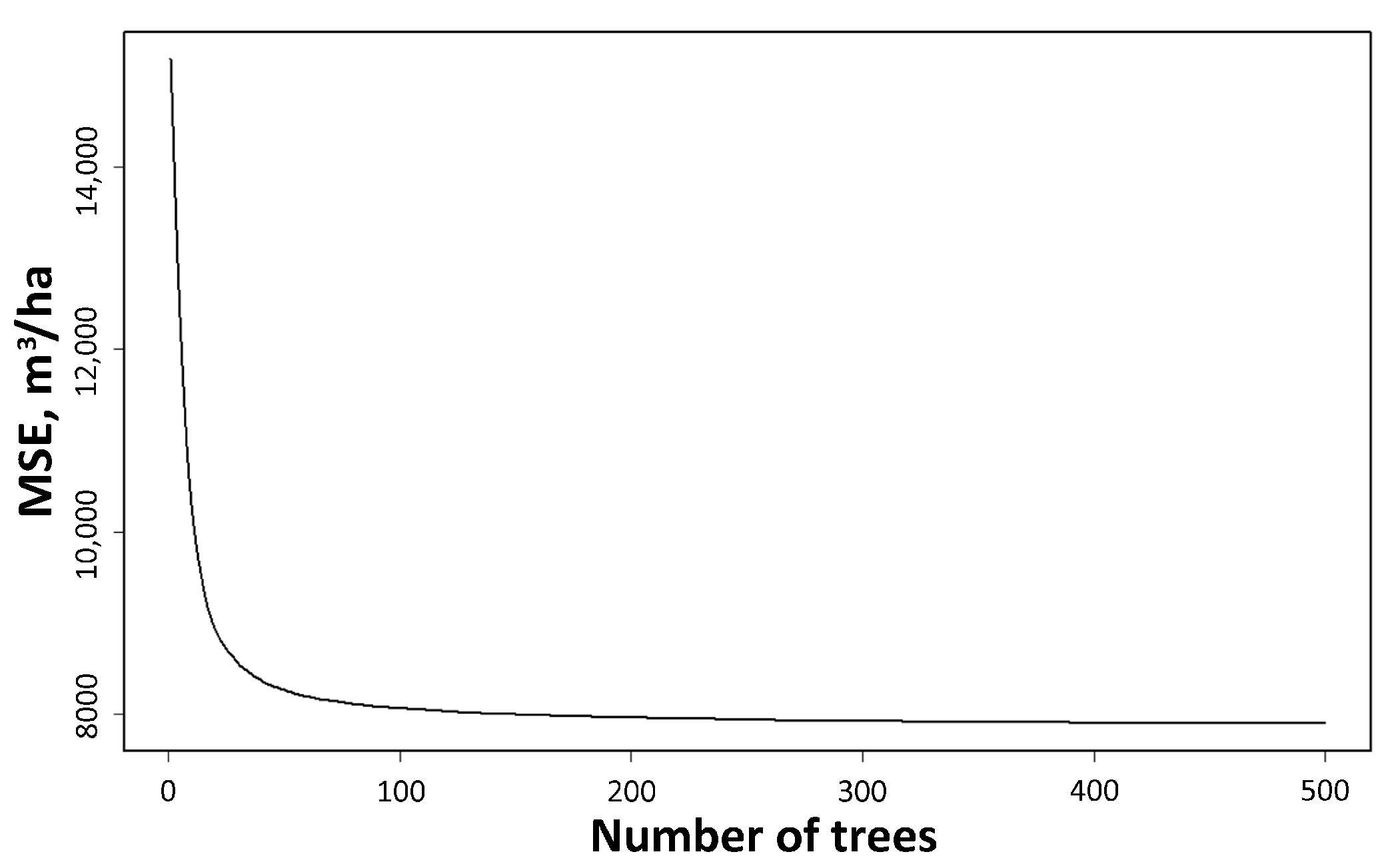
3.1. Random Forest Classifier
3.2. GSV Modeling
4. Results
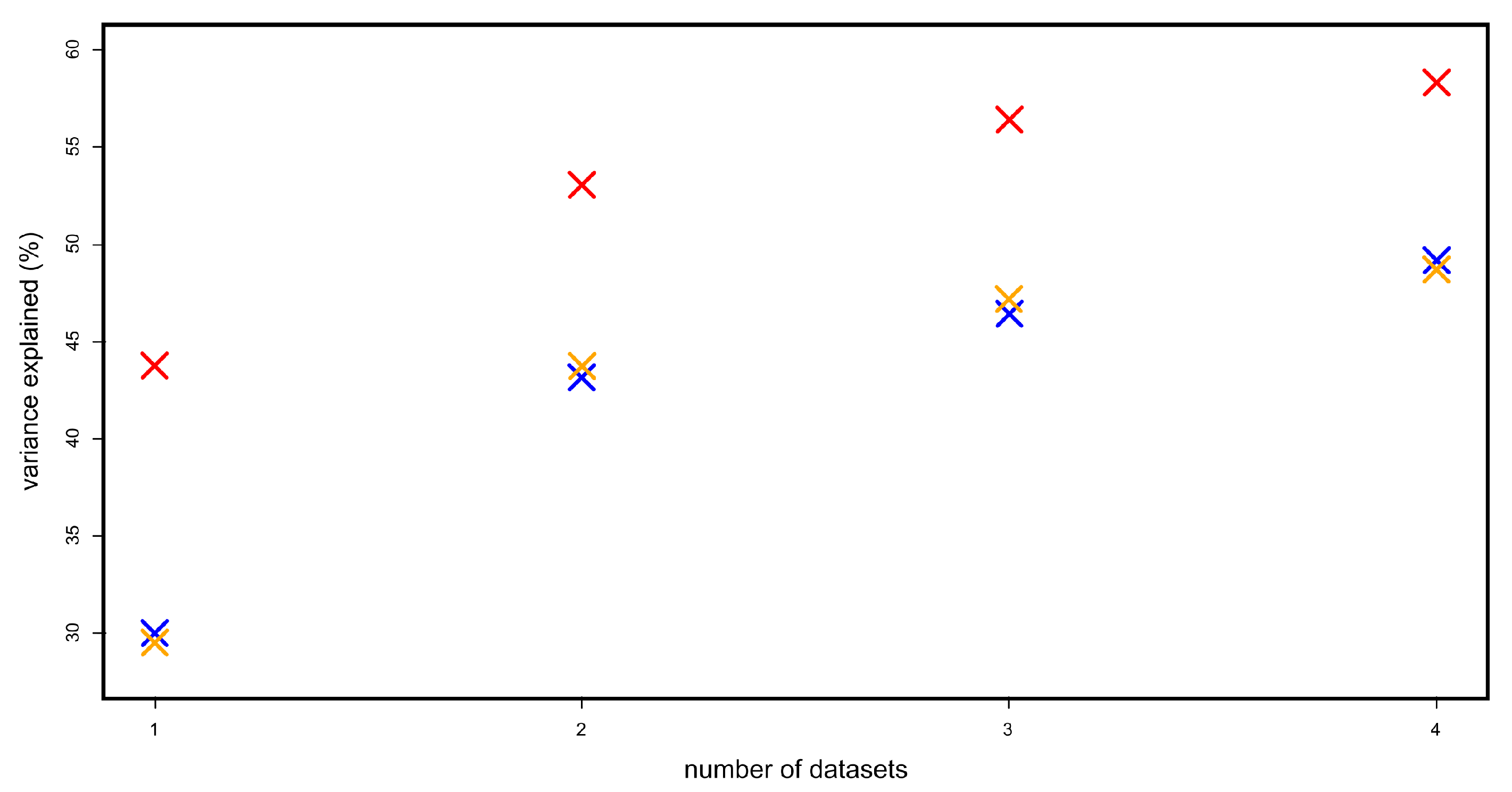
4.1. Random Forest Performance


| Year | 2007 | 2008 | 2009 | 2010 | Multi-Temporal |
|---|---|---|---|---|---|
| Variance explained | 29.83% | 32.33% | 29.92% | 30.14% | 46.63% |

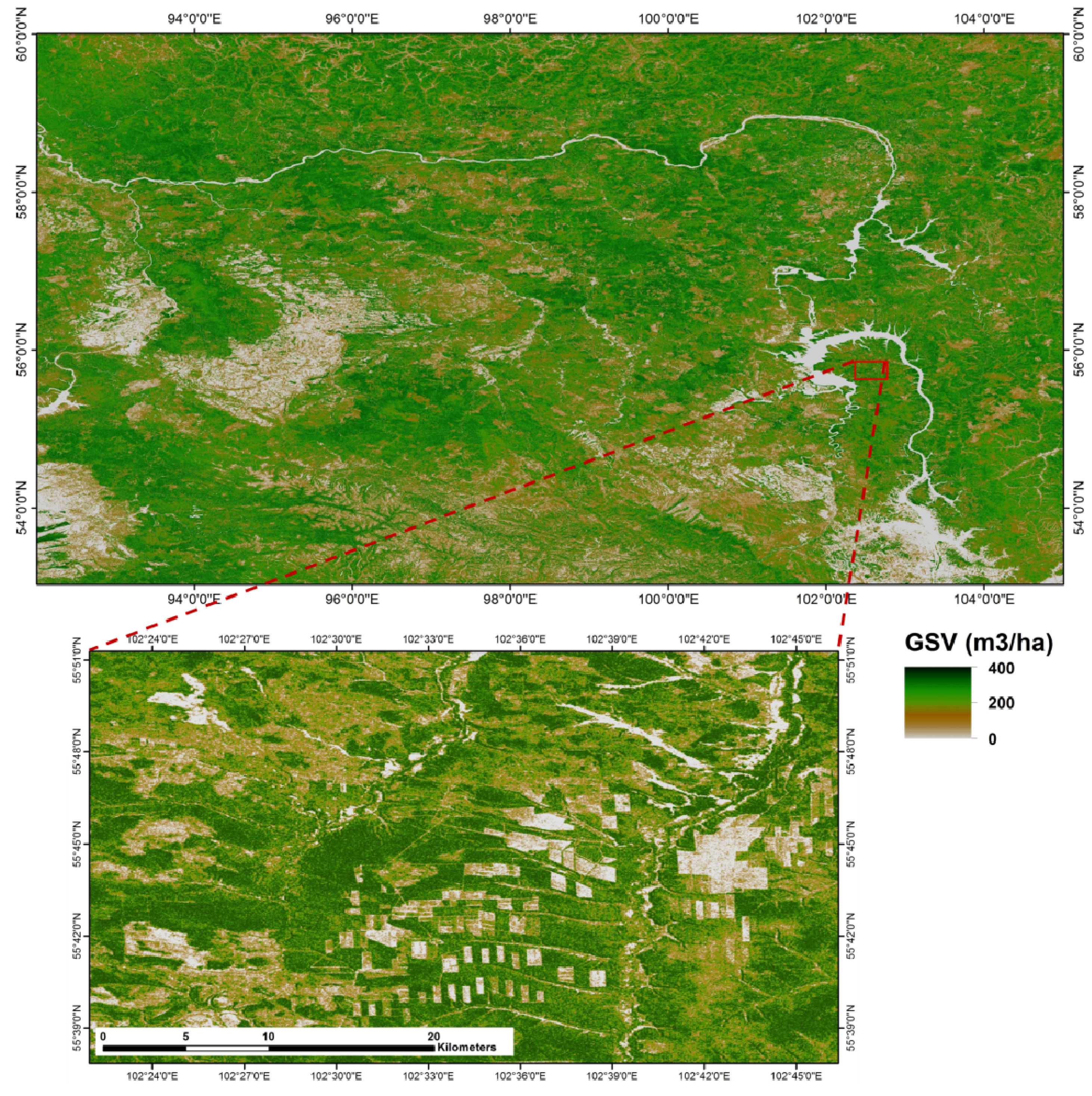
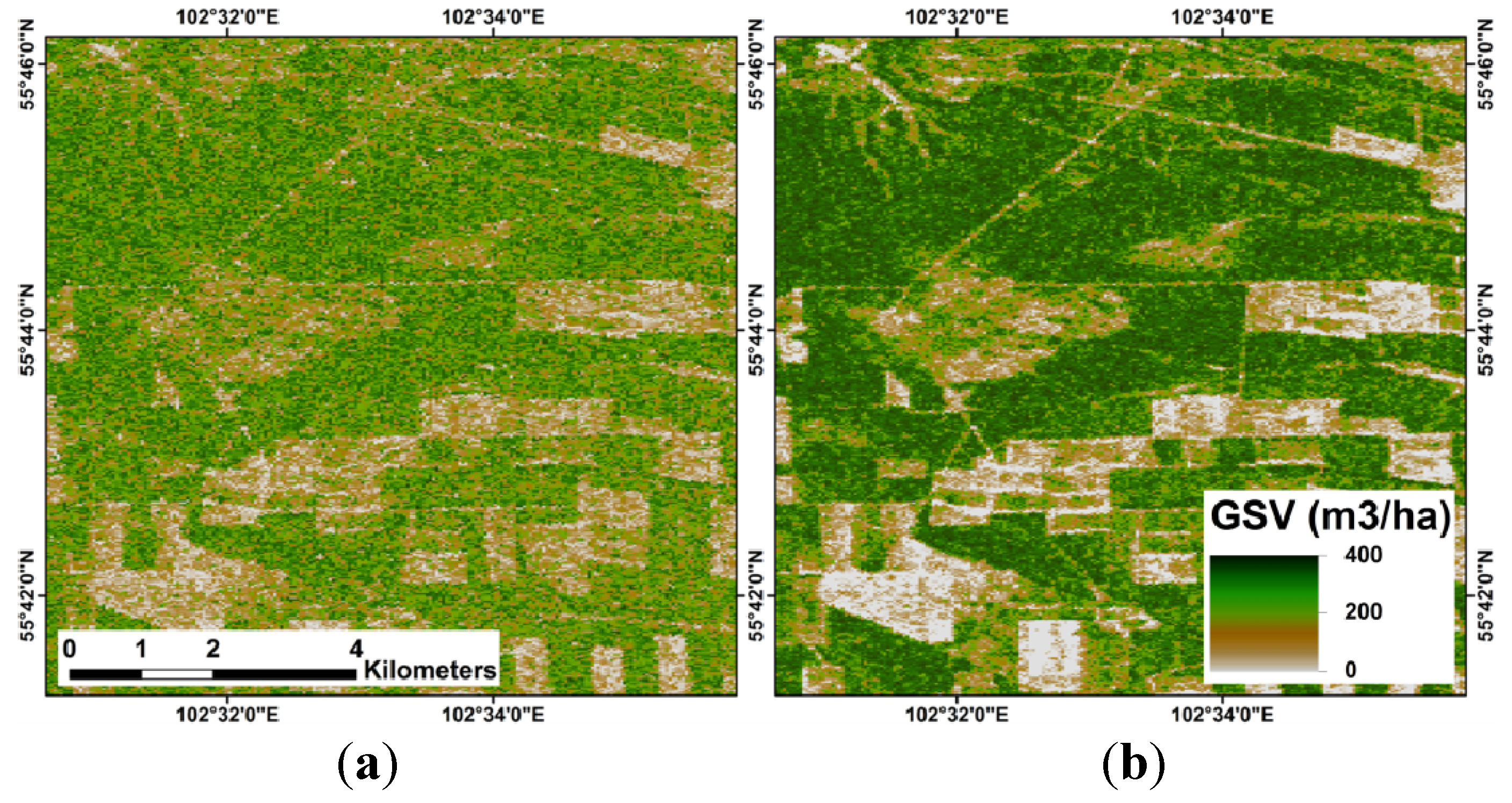
4.2. Mapping Results

| Year | 2007 | 2008 | 2009 | 2010 | Multi-Temporal |
|---|---|---|---|---|---|
| Range | 0–412 | 0–401 | 0–408 | 0–421 | 0–409 |


4.3. Validation
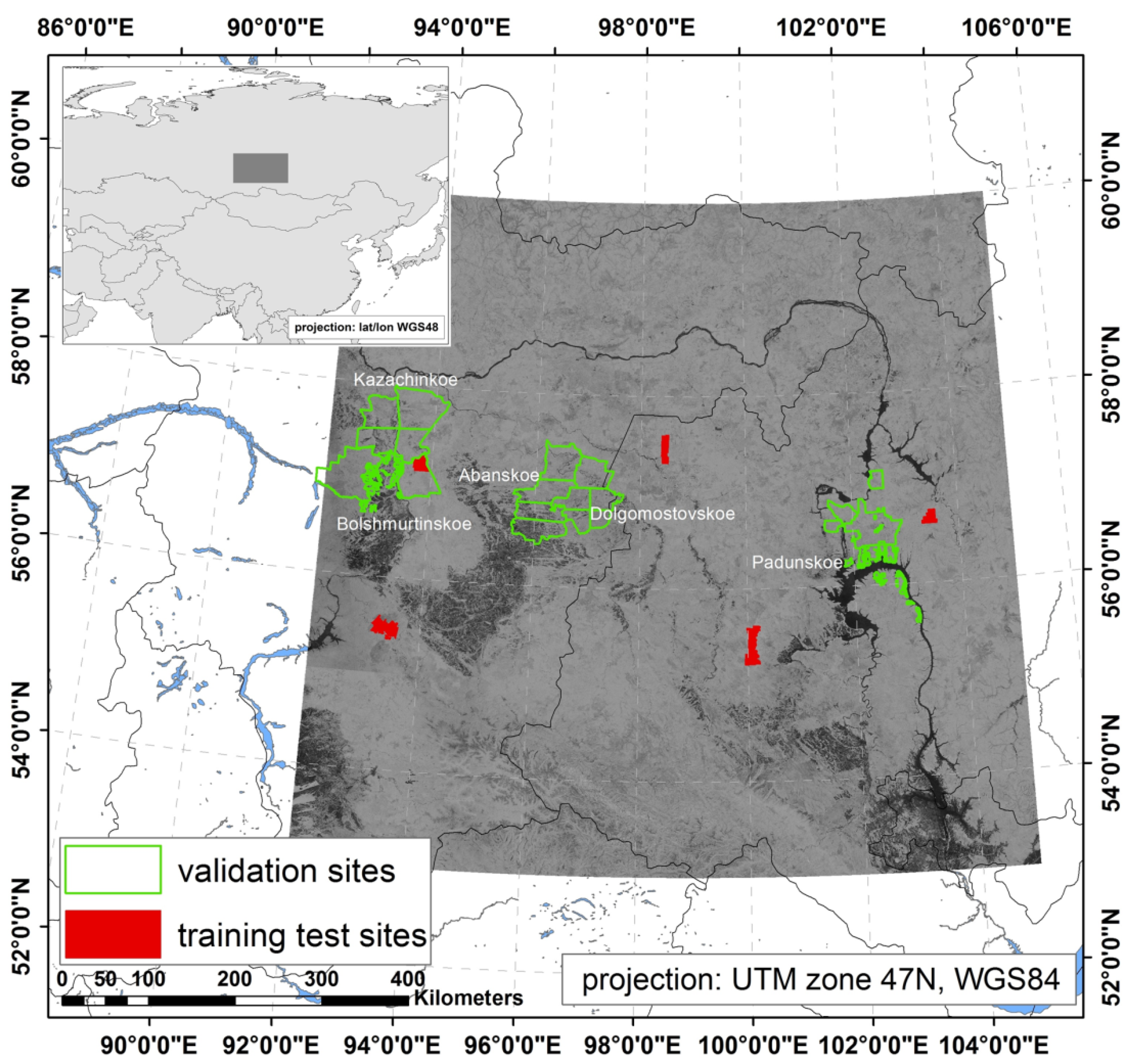
| Site number | Site Name (FMA Name) | Area, ha | FIP Number | Region |
|---|---|---|---|---|
| 1 | Kazachinskoe and Bolshemurtinskoe | 903,573 | 47,962 | Krasnoyarsk kray |
| 2 | Abanskoe and Dolgomostovskoe | 698,479 | 41,241 | Krasnoyarsk kray |
| 3 | Padunskoe | 366,696 | 22,318 | Irkutsk oblast |
| Total for all test sites | 1,968,748 | 111,521 |
| Label | Characteristics | 2007 | 2008 | 2009 | 2010 | Multi-Temporal |
|---|---|---|---|---|---|---|
| Emin | ∆ GSVmin | −259.1 | −249.6 | −264.9 | −285.8 | −247.9 |
| Emax | ∆ GSVmax | 202.5 | 216.5 | 217.6 | 208 | 221.2 |
| ME | Mean ∆ GSV (SAR-FI) | −1.3 | 1.4 | 6.3 | −14.6 | 3.7 |
| SD | ∆ GSV SD | 55.3 | 55.2 | 57.6 | 61.6 | 54.3 |
| RMSE | Root Mean Square Error | 55.3 | 55.2 | 57.9 | 63.3 | 54.4 |

| Dominant tree species | Emin | Emax | ME | SD | RMSE |
|---|---|---|---|---|---|
| Aspen | −184.3 | 210.7 | −5.9 | 56.3 | 56.6 |
| Birch | −170.0 | 186.7 | 21.1 | 46.5 | 51.1 |
| Fir | −270.0 | 221.2 | 29.2 | 72.0 | 72.1 |
| Larch | −171.1 | 131.2 | −3.4 | 45.2 | 45.3 |
| Pine | −247.9 | 193.6 | −16.9 | 58.0 | 60.4 |
| Siberian Pine | −310.0 | 209.0 | −39.1 | 63.3 | 74.4 |
| Spruce | −260.0 | 219.5 | 9.9 | 51.4 | 52.4 |
5. Discussion
6. Conclusions and Outlook
Acknowledgments
Author Contributions
Conflict of Interest
References
- Eriksson, L.E.B.; Santoro, M.; Wiesmann, A.; Schmullius, C.C. Multitemporal JERS repeat-pass coherence for growing-stock volume estimation of Siberian forest. IEEE Trans. Geosci. Remote Sens. 2003, 41, 1561–1570. [Google Scholar] [CrossRef]
- Dolman, A.J.; Shvidenko, A.; Schepaschenko, D.; Ciais, P.; Tchebakova, N.; Chen, T.; van der Molen, M.K.; Marchesini, L.B.; Maximov, T.C.; Maksyutov, S.; et al. An estimate of the terrestrial carbon budget of Russia using inventory-based, eddy covariance and inversion methods. Biogeosciences 2012, 9, 5323–5340. [Google Scholar] [CrossRef] [Green Version]
- Thiel, C.J.; Thiel, C.; Schmullius, C.C. Operational Large-Area Forest Monitoring in Siberia Using ALOS PALSAR Summer Intensities and Winter Coherence. IEEE Trans. Geosci. Remote Sens. 2009, 47, 3993–4000. [Google Scholar] [CrossRef]
- Hüttich, C.; Schmullius, C.C.; Thiel, C.J.; Pathe, C.; Bartalev, S.; Emelyanov, K.; Korets, M.; Shvidenko, A.; Schepaschenko, D. ZAPÁS: Assessment and monitoring of forest resources in the framework of the EU-Russia space dialogue. In Let’s Embrace Space, Volume Ⅱ—Space Research achievements under the 7th Framework Programme; Directorate-General for Enterprise and Industry, European Commission: Luxembourg, 2012; pp. 164–171. [Google Scholar]
- Beaudoin, A.; Toan, T.L.E.; Goze, S.; Nezry, E.; Lopes, A.; Mougin, E.; Hsu, C.C. Retrieval of forest biomass from SAR data. Int. J. Remote Sens. 1994, 15, 2777–2796. [Google Scholar] [CrossRef]
- Wang, Y.; Davis, F.W.; Melack, J.M.; Kasischke, E.S.; Christensen, N.L. The effects of changes in forest biomass on radar backscatter from tree canopies. Int. J. Remote Sens. 1995, 16, 503–513. [Google Scholar]
- Santoro, M.; Shvidenko, A.; Mccallum, I.; Askne, J.; Schmullius, C. Properties of ERS-1/2 coherence in the Siberian boreal forest and implications for stem volume retrieval. Remote Sens. Environ. 2007, 106, 154–172. [Google Scholar] [CrossRef]
- Ni, W.; Sun, G.; Member, S.; Guo, Z.; Zhang, Z.; He, Y. Retrieval of forest biomass from ALOS PALSAR data using a lookup table method. IEEE J. Sel. Top. Appl. Earth Obs. Remote Sens. 2013, 6, 875–886. [Google Scholar]
- Pulliainen, J.T.; Kurvonen, L.; Hallikainen, M.T. Multitemporal behavior of L- and C-band SAR observations of boreal forests. IEEE Trans. Geosci. Remote Sens. 1999, 37, 927–937. [Google Scholar]
- Rignot, E.; Way, J.; Williams, C.; Viereck, L. Radar estimates of aboveground biomass in boreal forests of interior Alaska. IEEE Trans. Geosci. Remote Sens. 1994, 32, 1117–1124. [Google Scholar] [CrossRef]
- Santoro, M.; Beer, C.; Cartus, O.; Schmullius, C.; Shvidenko, A.; McCallum, I.; Wegmüller, U.; Wiesmann, A. Retrieval of growing stock volume in boreal forest using hyper-temporal series of Envisat ASAR ScanSAR backscatter measurements. Remote Sens. Environ. 2011, 115, 490–507. [Google Scholar] [CrossRef]
- Dobson, M.; Ulaby, F.T.; LeToan, T.; Beaudoin, A.; Kasischke, E.S.; Christensen, N. Dependence of radar backscatter on coniferous forest biomass. IEEE Trans. Geosci. Remote Sens. 1992, 30, 412–415. [Google Scholar]
- Santoro, M.; Eriksson, L.; Askne, J.; Schmullius, C. Assessment of stand-wise stem volume retrieval in boreal forest from JERS-1 L-band SAR backscatter. Int. J. Remote Sens. 2006, 27, 3425–3454. [Google Scholar] [CrossRef]
- Sarker, M.L.R.; Nichol, J.; Ahmad, B.; Busu, I.; Rahman, A.A. Potential of texture measurements of two-date dual polarization PALSAR data for the improvement of forest biomass estimation. ISPRS J. Photogramm. Remote Sens. 2012, 69, 146–166. [Google Scholar] [CrossRef]
- Harrell, P.A.; Bourgeau-Chavez, L.L.; Kasischke, E.S.; French, N.H.F.; Christensen, N.L. Sensitivity of ERS-1 and JERS-1 radar data to biomass and stand structure in Alaskan boreal forest. Remote Sens. Environ. 1995, 54, 247–260. [Google Scholar]
- Fransson, J.E.S.; Israelsson, H. Estimation of stem volume in boreal forests using ERS-1 C- and JERS-1 L- band SAR data. Int. J. Remote Sens. 1990, 20, 123–137. [Google Scholar] [CrossRef]
- Rauste, Y. Multi-temporal JERS SAR data in boreal forest biomass mapping. Remote Sens. Environ. 2005, 97, 263–275. [Google Scholar] [CrossRef]
- Luckman, A.; Baker, J.; Honza, M.; Lucas, R. Tropical forest biomass density estimation using JERS-1 SAR: Seasonal variation, confidence limits, and application to image mosaics. Remote Sens. Environ. 1998, 63, 126–139. [Google Scholar] [CrossRef]
- Lucas, R.; Armston, J.; Fairfax, R.; Fensham, R.; Accad, A.; Carreiras, J.; Kelley, J.; Bunting, P.; Clewley, D.; Bray, S.; et al. An evaluation of the ALOS PALSAR L-band backscatter—Above ground biomass relationship Queensland, Australia: Impacts of surface moisture condition and vegetation structure. IEEE J. Sel. Top. Appl. Earth Obs. Remote Sens. 2010, 3, 576–593. [Google Scholar]
- Rosenqvist, A.; Shimada, M.; Ito, N.; Watanabe, M. ALOS PALSAR: A pathfinder mission for global-scale monitoring of the environment. IEEE Trans. Geosci. Remote Sens. 2007, 45, 3307–3316. [Google Scholar] [CrossRef]
- Ogawa, T.; Shimada, M.; Igarashi, T. Initiating the ALOS Kyoto & carbon initiative. In Proceedings of the IEEE 2001 International Geoscience and Remote Sensing Symposium (IGARSS), Sydney, NSW, Austrilia, 9–13 July 2001; pp. 546–548.
- Shimada, M.; Ohtaki, T. Generating large-scale high-quality SAR mosaic datasets: Application to PALSAR data for global monitoring. IEEE J. Sel. Top. Appl. Earth Obs. Remote Sens. 2010, 3, 637–656. [Google Scholar]
- Breiman, L. Random forests. Mach. Learn. 2001, 45, 5–32. [Google Scholar] [CrossRef]
- Carreiras, J.M.B.; Pereira, J.M.C.; Shimabukuro, Y.E. Land-cover mapping in the Brazilian Amazon using SPOT-4 vegetation data and machine learning classification methods. Photogramm. Eng. Remote Sens. 2006, 72, 897–910. [Google Scholar] [CrossRef]
- Moisen, G.G.; Freeman, E.A.; Blackard, J.A.; Frescino, T.S.; Zimmermann, N.E.; Edwards, T.C. Predicting tree species presence and basal area in Utah: A comparison of stochastic gradient boosting, generalized additive models, and tree-based methods. Ecol. Model. 2006, 199, 176–187. [Google Scholar] [CrossRef]
- Carreiras, J.M.B.; Melo, J.B.; Vasconcelos, M.J. Estimating the above-ground biomass in Miombo Savanna woodlands (Mozambique, East Africa) using L-band synthetic aperture radar data. Remote Sens. 2013, 5, 1524–1548. [Google Scholar] [CrossRef]
- Breiman, L.; Friedman, J.H.; Olshen, R.A.; Stone, C.J. Classification and Regression Trees; Wadsworth: Pacific Grove, CA, USA, 1984; p. 368. [Google Scholar]
- Prasad, A.M.; Iverson, L.R.; Liaw, A. Newer classification and regression tree techniques: Bagging and random forests for ecological prediction. Ecosystems 2006, 9, 181–199. [Google Scholar] [CrossRef]
- Cutler, D.R.; Edwards, T.C.; Beard, K.H.; Cutler, A.; Hess, K.T.; Gibson, J.; Lawler, J.J. Random forests for classification in ecology. Ecology 2007, 88, 2783–2792. [Google Scholar] [CrossRef]
- Hüttich, C.; Herold, M.; Strohbach, B.J.; Dech, S. Integrating in-situ, Landsat, and MODIS data for mapping in Southern African savannas: Experiences of LCCS-based land-cover mapping in the Kalahari in Namibia. Environ. Monit. Assess. 2011, 176, 531–547. [Google Scholar] [CrossRef]
- Carreiras, J.M.B.; Pereira, J.M.C.; Campagnolo, M.L.; Shimabukuro, Y.E. Assessing the extent of agriculture/pasture and secondary succession forest in the Brazilian Legal Amazon using SPOT VEGETATION data. Remote Sens. Environ. 2006, 101, 283–298. [Google Scholar] [CrossRef]
- Houghton, R.A.; Butman, D.; Bunn, A.G.; Krankina, O.N.; Schlesinger, P.; Stone, T.A. Mapping Russian forest biomass with data from satellites and forest inventories. Environ. Res. Lett. 2007, 2. [Google Scholar] [CrossRef]
- Gislason, P.O.; Benediktsson, J.A.; Sveinsson, J.R. Random forests for land cover classification. Pattern Recognit. Lett. 2006, 27, 294–300. [Google Scholar] [CrossRef]
- Simard, M.; Pinto, N.; Fisher, J.B.; Baccini, A. Mapping forest canopy height globally with spaceborne lidar. J. Geophys. Res. 2011, 116, 1–12. [Google Scholar]
- Cartus, O.; Kellndorfer, J.; Rombach, M.; Walker, W. Mapping canopy height and growing stock volume using Airborne Lidar, ALOS PALSAR and Landsat ETM+. Remote Sens. 2012, 4, 3320–3345. [Google Scholar] [CrossRef]
- Liaw, A.; Wiener, M. Classification and regression by randomForest. R News 2002, 2, 18–22. [Google Scholar]
- Rauste, Y.; Hame, T.; Pulliainen, J.; Heiska, K.; Hallikainen, M. Radar-based forest biomass estimation. Int. J. Remote Sens. 1994, 15, 2797–2808. [Google Scholar] [CrossRef]
- Le Toan, T.; Beaudoin, A.; Riom, J.; Guyon, D. Relating forest biomass to SAR data. IEEE Trans. Geosci. Remote Sens. 1994, 30, 403–411. [Google Scholar]
- Sandberg, G.; Ulander, L.M.H.; Fransson, J.E.S.; Holmgren, J.; Le Toan, T. L- and P-band backscatter intensity for biomass retrieval in hemiboreal forest. Remote Sens. Environ. 2011, 115, 2874–2886. [Google Scholar] [CrossRef]
- Cartus, O.; Santoro, M.; Kellndorfer, J. Mapping forest aboveground biomass in the Northeastern United States with ALOS PALSAR dual-polarization L-band. Remote Sens. Environ. 2012, 124, 466–478. [Google Scholar] [CrossRef]
- Peregon, A.; Yamagata, Y. The use of ALOS/PALSAR backscatter to estimate above-ground forest biomass: A case study in Western Siberia. Remote Sens. Environ. 2013, 137, 139–146. [Google Scholar] [CrossRef]
- Harrell, P.A.; Kasischke, E.S.; Bourgeau-chavez, L.L.; Haney, E.M.; Christensen, N.L, Jr. Evaluation of approaches to estimating aboveground biomass in southern pine forests using SIR-C data. Remote Sens. Environ. 1997, 59, 223–233. [Google Scholar] [CrossRef]
- Kasischke, E.S.; Tanase, M.A.; Bourgeau-Chavez, L.L.; Borr, M. Soil moisture limitations on monitoring boreal forest regrowth using spaceborne L-band SAR data. Remote Sens. Environ. 2011, 115, 227–232. [Google Scholar] [CrossRef]
- Santoro, M.; Askne, J.; Eriksson, L.; Schmullius, C.; Wiesmann, A. Seasonal dynamics and stem volume retrieval in boreal forests using JERS-1 backscatter. Proc. SPIE 2002, 41, 231–242. [Google Scholar]
- Suzuki, R.; Kim, Y.; Ishii, R. Sensitivity of the backscatter intensity of ALOS/PALSAR to the above-ground biomass and other biophysical parameters of boreal forest in Alaska. Polar Sci. 2013, 7, 100–112. [Google Scholar] [CrossRef]
- De Grandi, G.D.; Bouvet, A.; Lucas, R.M.; Shimada, M.; Monaco, S.; Rosenqvist, A. The K&C PALSAR mosaic of the African continent: Processing issues and first thematic results. IEEE Trans. Geosci. Remote Sens. 2011, 49, 3593–3610. [Google Scholar] [CrossRef]
- Patenaude, G.; Milne, R.; Dawson, T.P. Synthesis of remote sensing approaches for forest carbon estimation: reporting to the Kyoto Protocol. Environ. Sci. Policy 2005, 8, 161–178. [Google Scholar] [CrossRef]
- Watanabe, M.; Shimada, M. Relation between coherence, forest biomass, and L-band σ0. In Proceedings of the IEEE International Conference on International Geoscience and Remote Sensing Symposium (IGARSS), Denver, CO, USA, 31 July–4 August 2006; pp. 1651–1654.
- Gaveau, D.L.A.; Balzter, H.; Plummer, S. Forest woody biomass classification with satellite-based radar coherence over 900 000 km2 in Central Siberia. Forest Ecol. Management 2003, 174, 65–75. [Google Scholar] [CrossRef]
- Okada, Y.; Hamasaki, T.; Tsuji, M.; Iwamato, M.; Hariu, K.; Kankaku, Y.; Suzuki, S.; Osawa, Y. Hardware performance of L-band SAR system onboard ALOS-2. In Proceedings of the 2001 IEEE International Geoscience and Remote Sensing Symposium (IGARSS), Vancouver, BC, Canada, 24–29 July 2011; pp. 894–897.
© 2014 by the authors; licensee MDPI, Basel, Switzerland. This article is an open access article distributed under the terms and conditions of the Creative Commons Attribution license (http://creativecommons.org/licenses/by/3.0/).
Share and Cite
Wilhelm, S.; Hüttich, C.; Korets, M.; Schmullius, C. Large Area Mapping of Boreal Growing Stock Volume on an Annual and Multi-Temporal Level Using PALSAR L-Band Backscatter Mosaics. Forests 2014, 5, 1999-2015. https://doi.org/10.3390/f5081999
Wilhelm S, Hüttich C, Korets M, Schmullius C. Large Area Mapping of Boreal Growing Stock Volume on an Annual and Multi-Temporal Level Using PALSAR L-Band Backscatter Mosaics. Forests. 2014; 5(8):1999-2015. https://doi.org/10.3390/f5081999
Chicago/Turabian StyleWilhelm, Sebastian, Christian Hüttich, Mikhail Korets, and Christiane Schmullius. 2014. "Large Area Mapping of Boreal Growing Stock Volume on an Annual and Multi-Temporal Level Using PALSAR L-Band Backscatter Mosaics" Forests 5, no. 8: 1999-2015. https://doi.org/10.3390/f5081999