
Decision Support Systems (DSS) Optimal—A Case Study from the Czech Republic


Abstract
:1. Introduction
2. Material and Methods
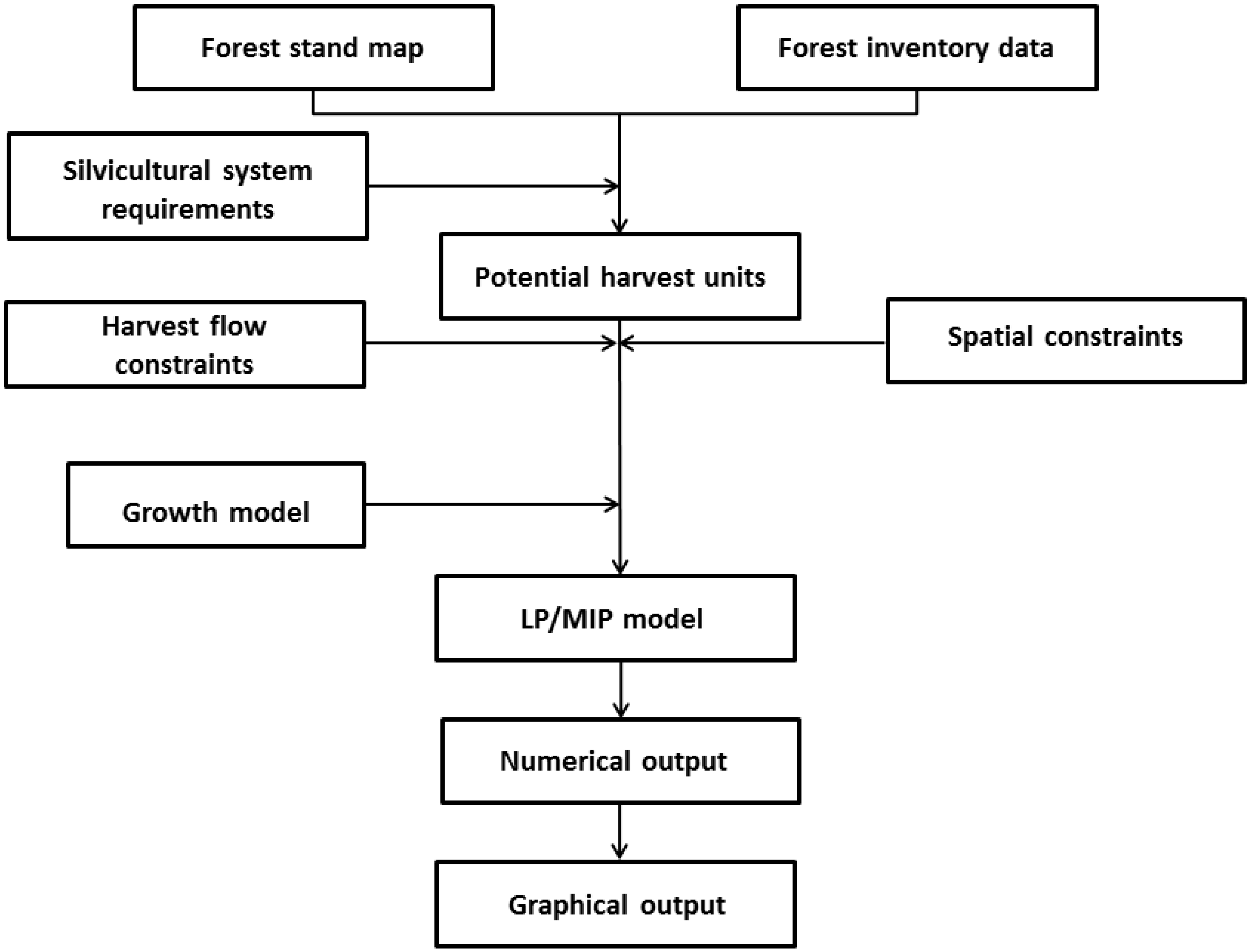
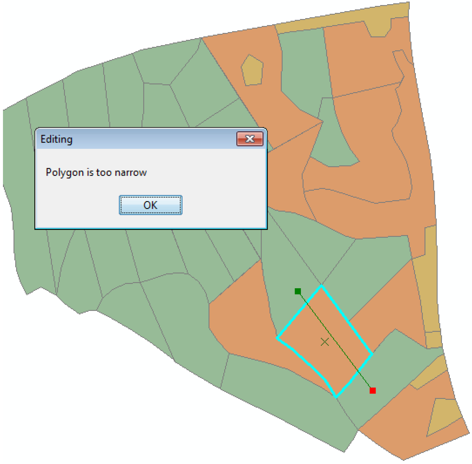
2.1. DSS Optimal


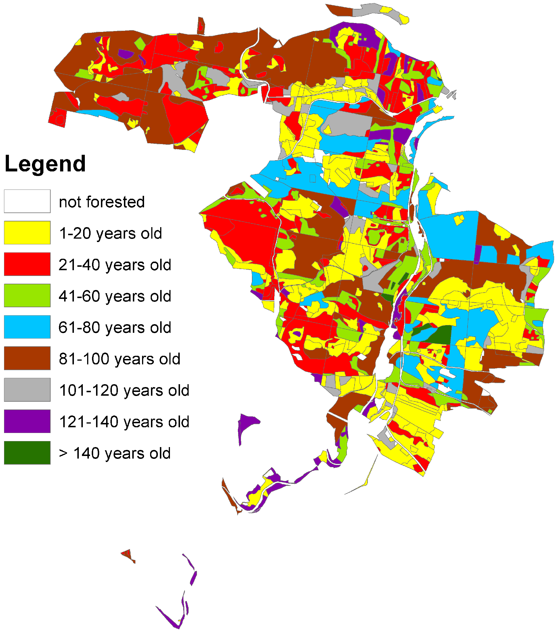
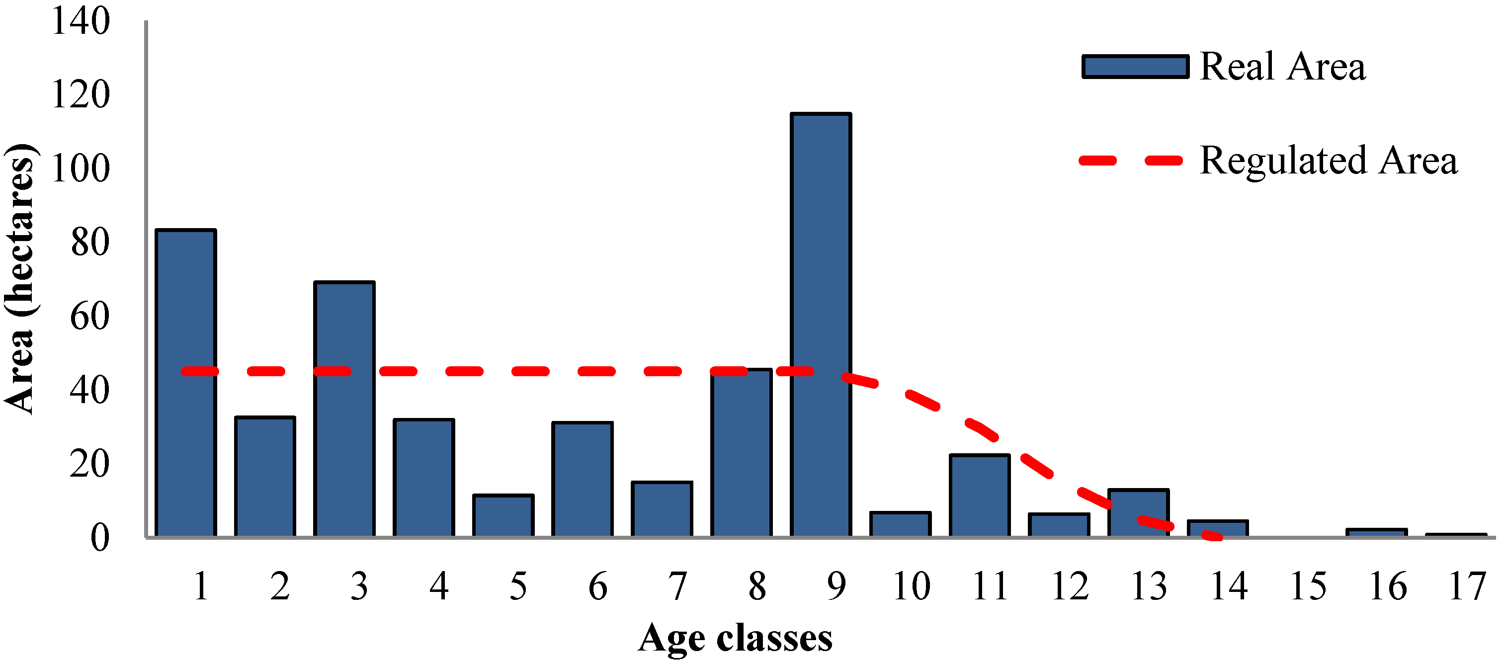
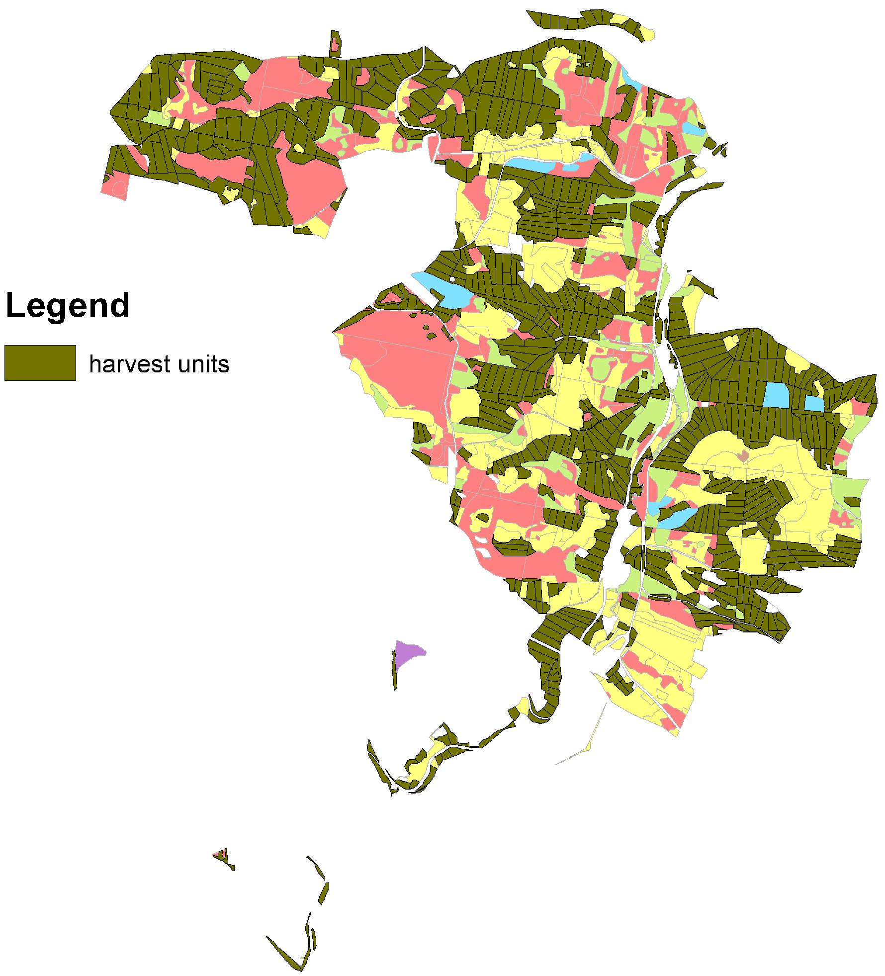
2.2. Case Study


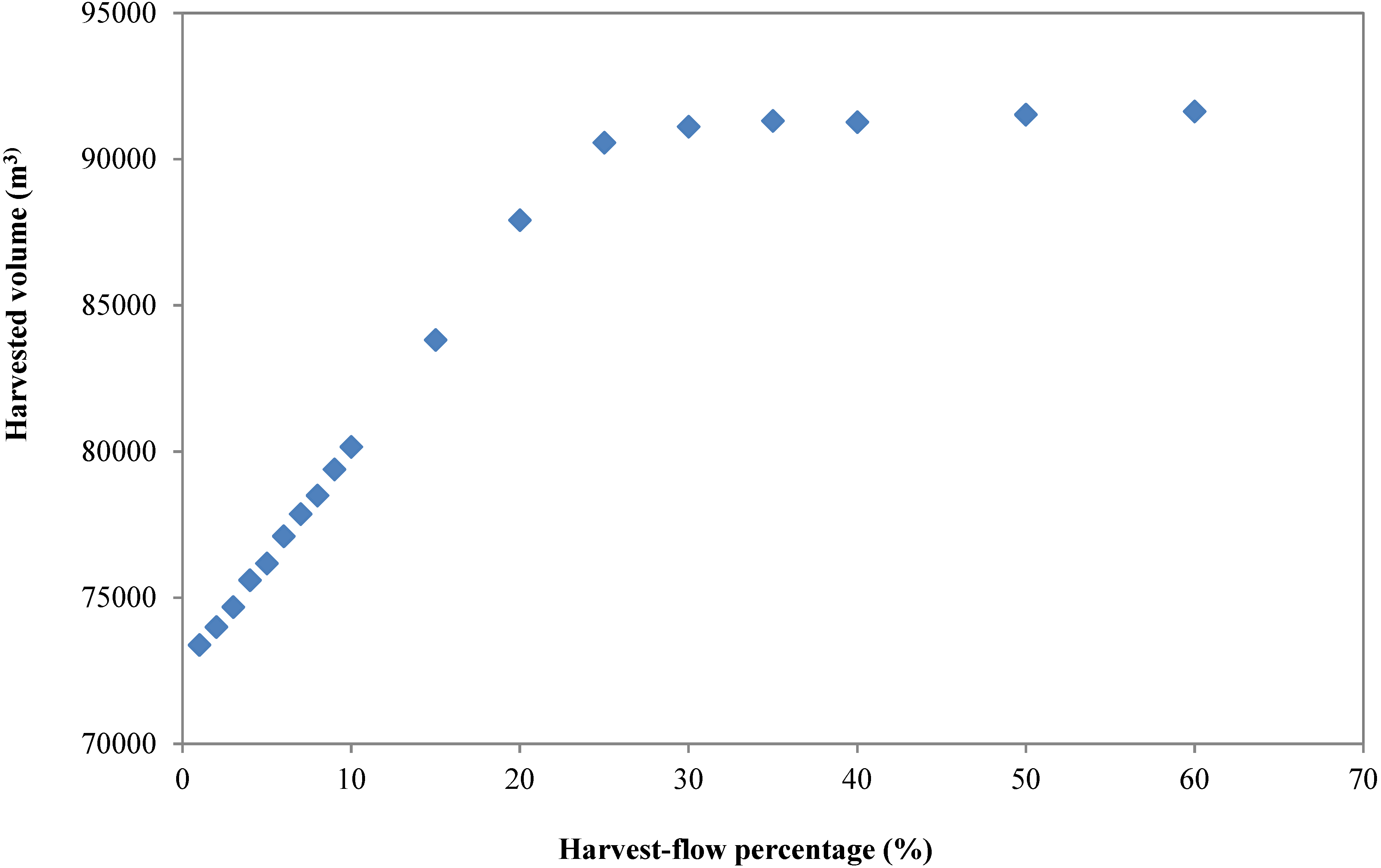
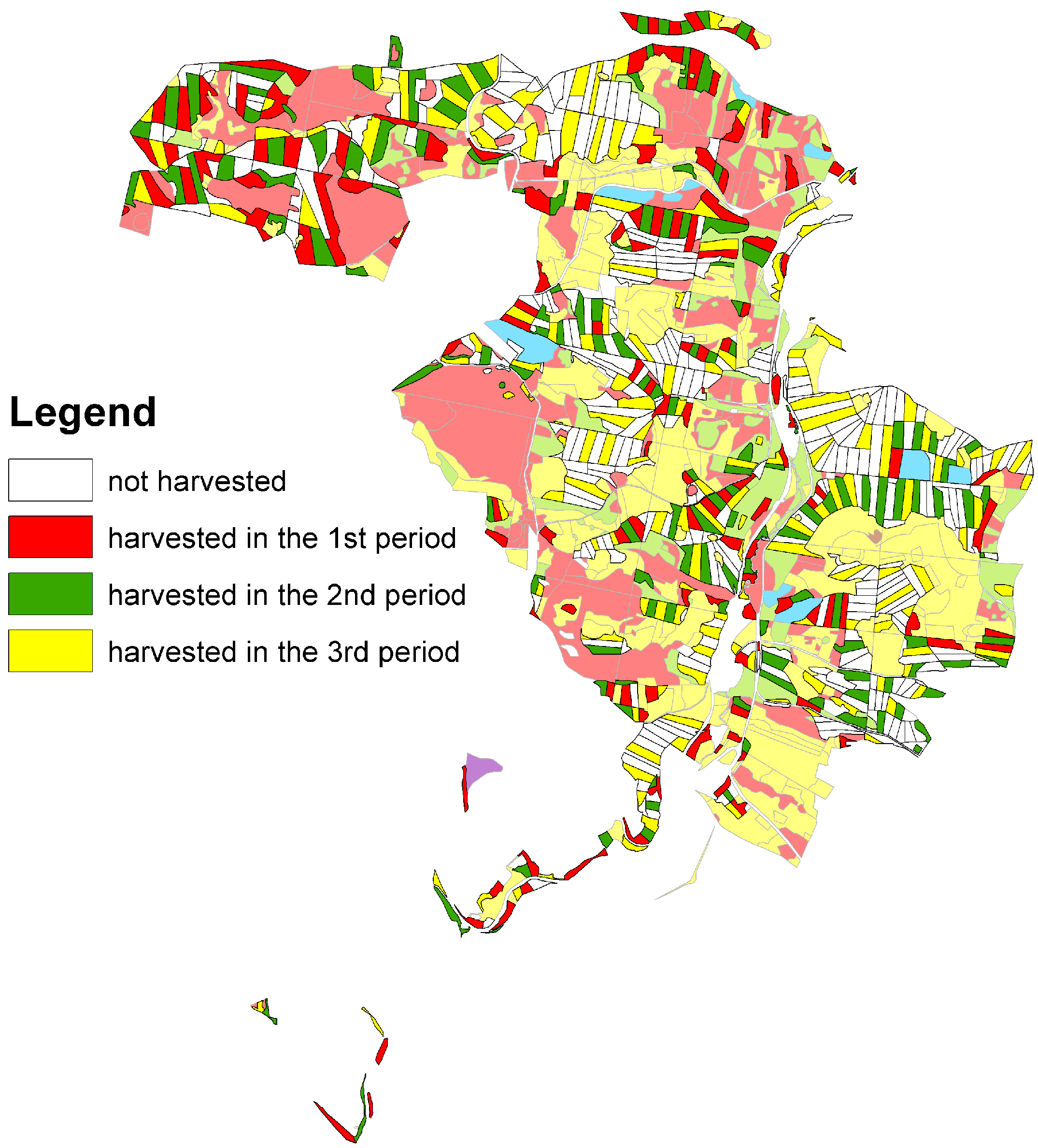
3. Results and Discussion

| Total Harvested Amount (m3) | Harvest in 1st Period (m3) | Harvest in 2nd Period (m3) | Harvest in 3rd Period (m3) |
|---|---|---|---|
| 102,032 | 31,824 | 32,598 | 37,610 |
| Gap tolerance | Resulted gap | Total harvested amount (m3) | Harvest in 1st period (m3) | Harvest in 2nd period (m3) | Harvest in 3rd period (m3) | Elapsed time of solver (s) | Elapsed time of Optimal (s) |
|---|---|---|---|---|---|---|---|
| The harvest flow difference 10% | |||||||
| 1.00 × 10⁻⁴ | 0.0022% | 80,157 | 24,217 | 26,638 | 29,302 | 0.45 | 242 |
| 1.00 × 10⁻³ | 0.0517% | 80,157 | 24,217 | 26,638 | 29,302 | 0.40 | 230 |
| 1.00 × 10⁻² | 0.7606% | 79,701 | 24,101 | 26,450 | 29,150 | 0.34 | 230 |
| 1.00 × 10⁻¹ | 7.8183% | 76,182 | 23,016 | 25,317 | 27,849 | 0.25 | 233 |
| The harvest flow difference 20% | |||||||
| 1.00× 10⁻⁴ | 0.0036% | 88,051 | 24,183 | 29,031 | 34,837 | 1.57 | 236 |
| 1.00× 10⁻³ | 0.0562% | 88,029 | 24,193 | 29,018 | 34,818 | 0.55 | 235 |
| 1.00× 10⁻² | 0.5092% | 87,910 | 24,154 | 28,980 | 34,776 | 0.41 | 245 |
| 1.00× 10⁻¹ | 9.1537% | 82,753 | 22,737 | 27,280 | 32,736 | 0.27 | 232 |
| The harvest flow difference 30% | |||||||
| 1.00× 10⁻⁴ | 0.0007% | 91,216 | 22,867 | 29,722 | 38,627 | 2.24 | 244 |
| 1.00× 10⁻³ | 0.0530% | 91,216 | 22,870 | 29,724 | 38,622 | 1.97 | 239 |
| 1.00× 10⁻² | 0.6636% | 91,108 | 22,877 | 29,674 | 38,557 | 0.50 | 240 |
| 1.00× 10⁻¹ | 9.6607% | 87,141 | 21,882 | 28,375 | 36,884 | 0.21 | 234 |
| Gap tolerance | Resulted gap | Total harvested amount (m3) | Harvest in 1st period (m3) | Harvest in 2nd period (m3) | Harvest in 3rd period (m3) | Elapsed time of solver (s) | Elapsed time of Optimal (s) |
|---|---|---|---|---|---|---|---|
| The harvest flow difference 10% | |||||||
| 1.00× 10⁻⁴ | 0.0089% | 94,782 | 28,635 | 31,499 | 34,648 | 0.42 | 2557 |
| 1.00× 10⁻³ | 0.0298% | 94,778 | 28,635 | 31,497 | 34,646 | 0.36 | 2470 |
| 1.00× 10⁻² | 0.8973% | 94,309 | 28,494 | 31,341 | 34,474 | 0.27 | 2677 |
| 1.00× 10⁻¹ | 8.9499% | 92,202 | 27,856 | 30,641 | 33,705 | 0.18 | 2531 |
| The harvest flow difference 20% | |||||||
| 1.00× 10⁻⁴ | 0.0097% | 104,231 | 28,635 | 34,362 | 41,234 | 0.58 | 2581 |
| 1.00× 10⁻³ | 0.0097% | 104,231 | 28,635 | 34,362 | 41,234 | 0.59 | 2624 |
| 1.00× 10⁻² | 0.8624% | 103,384 | 28,404 | 34,082 | 40,898 | 0.49 | 2560 |
| 1.00× 10⁻¹ | 5.4827% | 99,665 | 27,382 | 32,856 | 39,427 | 0.28 | 2591 |
| The harvest flow difference 30% | |||||||
| 1.00× 10⁻⁴ | 0.0015% | 108,675 | 27,239 | 35,408 | 46,028 | 7.68 | 2613 |
| 1.00× 10⁻³ | 0.0948% | 108,675 | 27,239 | 35,408 | 46,028 | 3.76 | 2634 |
| 1.00× 10⁻² | 0.5647% | 108,436 | 27,188 | 35,330 | 45,918 | 0.53 | 2547 |
| 1.00× 10⁻¹ | 7.9413% | 103,564 | 26,112 | 33,676 | 43,776 | 0.18 | 2841 |
| Harvest Flow Difference | Total Harvested Volume (m3) | Harvest in 1st Period (m3) | Harvest in 2nd Period (m3) | Harvest in 3rd Period (m3) |
|---|---|---|---|---|
| 10% | 136,326 | 41,190 | 45,303 | 49,833 |
| 20% | 136,827 | 37,612 | 45,098 | 54,117 |
| 30% | 137,260 | 34,440 | 44,705 | 58,115 |
| Total Harvested Amount (m3) | Harvest in 1st Period (m3) | Harvest in 2nd Period (m3) | Harvest in 3rd Period (m3) | |
|---|---|---|---|---|
| AdC-M | 92,806 | 12,083 | 29,799 | 50,204 |
| AdC-N | 110,200 | 8,111 | 34,568 | 67,521 |


4. Conclusions
Acknowledgments
Author Contributions
Appendix
Mathematical Formulation
Java programming code for the model transferring to Gurobi
package com.proforesters.solver;
/**
* @author kaspar
*
*/
import gurobi.GRB;
import gurobi.GRBEnv;
import gurobi.GRBException;
import gurobi.GRBLinExpr;
import gurobi.GRBModel;
import gurobi.GRBVar;
import com.esri.arcgis.geodatabase.IFeatureClass;
import com.proforesters.optimal.OptimalExtension;
public class ClearCutSystemSolver {
       public static double[] getSolution (int [][] matrix, int periodCount, int deviation, double [] [] objectiveMatrix, int [] patches, IFeatureClass featureClass, int [][] timeHarvest, int gapTolerance) {
          double [] results = new double [periodCount * matrix.length];
          try{
          GRBEnv env = new GRBEnv("mip1.log");
          GRBModel model = new GRBModel(env);
          double gT = gapTolerance * 1000
          double doubleGapTolerance = gT/ 10000000;
          model.getEnv().set(GRB.DoubleParam.MIPGap,doubleGapTolerance);
          double decimalDeviation =((double)deviation)/100;
          int finalCountOfRow = matrix.length * periodCount + matrix.length  +(2*periodCount − 2) + 1;
          int [] finalConstraints = new int [finalCountOfRow];
          int [] sumRow = new int [matrix.length];
          int [] diagElem = new int [matrix.length];
          for (int i = 0; i < matrix.length; i++) {
           for (int j = 0; j < matrix.length; j++) {
            sumRow [i] += (matrix [i][j]);}}
          for (int i = 0; i < matrix.length; i++) {
           diagElem [i] = (sumRow [i])/2;}
          for (int i = 0; i < periodCount; i++) {
           for (int j = 0; j < matrix.length; j++) {
            finalConstraints [i*matrix.length+j] = diagElem [j];}}
          for (int i = matrix.length * periodCount; i < matrix.length *  periodCount + 2 * periodCount − 2; i++) {
           finalConstraints [i] = 0;}
          for (int i = matrix.length * periodCount + 2 * periodCount − 2; i < finalCountOfRow − 1; i++) {
           finalConstraints [i] = 1;}
          int sumOfPatchesVector=0;
          for (int i = 0; i < patches.length; i++) {
           sumOfPatchesVector += patches [i];}
          for (int i = finalCountOfRow − 1; i < finalCountOfRow; i++) {
           finalConstraints [i] = sumOfPatchesVector;}
          int n = matrix.length * periodCount;
          GRBVar [] x = new GRBVar[n];
          for (int i = 0; i < matrix.length * periodCount; i++) {
           String st = "x" + String.valueOf(i);
           x[i] = model.addVar(0.0, 1.0, 0.0, GRB.BINARY, st);}
          model.update();
          double [] objectiveVector = new double [periodCount * matrix.length];
          for (int i = 0; i < periodCount; i++) {
           for (int j = 0; j < matrix.length; j++){
            objectiveVector [j+i*matrix.length] = objectiveMatrix [i][j];}}
          GRBLinExpr expr = new GRBLinExpr();
          for (int i = 0; i < matrix.length * periodCount; i++) {
           expr.addTerm(objectiveVector[i], x[i]);}
          model.setObjective(expr, GRB.MAXIMIZE);
          int count = matrix.length*periodCount;
          for(int i = 0; i < periodCount;i++){
           for (int j = 0; j < matrix.length; j++) {
            expr = new GRBLinExpr();
             for (int k = 0; k < matrix.length; k++) {
              expr.addTerm(matrix[j][k], x[(matrix.length * i) + k]);}
             String st = "c" +    String.valueOf((matrix.length * i) + j);
            model.addConstr(expr, GRB.LESS_EQUAL, finalConstraints[j], st);}}
          double [][] evenFlowMatrixUP = new double [periodCount-1][matrix.length * periodCount];
          for (int i = 0; i < periodCount − 1; i++) {
           for (int j = 0; j < matrix.length * periodCount; j++){
            evenFlowMatrixUP [i][j] = 0;}}
          for (int i = 0; i < periodCount −+− 1; i++) {
           for (int j = 0; j < matrix.length; j++) {
            evenFlowMatrixUP [i][i*matrix.length+j] = −(1 + decimalDeviation) * objectiveMatrix [i][j];}}
          for (int i = 1; i < periodCount; i++) {
           for (int j = 0; j < matrix.length; j++) {
            evenFlowMatrixUP [i − 1][i*matrix.length + j] = objectiveMatrix [i][j];}}
          for (int i = matrix.length * periodCount; i < matrix.length * periodCount +(periodCount – 1); i++) {
           expr = new GRBLinExpr();
           for (int j = 0; j < matrix.length * periodCount; j++) {
            expr.addTerm(evenFlowMatrixUP[i - (matrix.length * periodCount)][j], x[j]);}
           String st = "c" + String.valueOf(i);
           model.addConstr(expr, GRB.LESS_EQUAL, finalConstraints[i], st);}
          double [][] evenFlowMatrixLO = new double [periodCount-1][matrix.length * periodCount];
          for (int i = 0; i < periodCount − 1; i++) {
           for (int j = 0; j < matrix.length * periodCount; j++){
            evenFlowMatrixLO [i][j] = 0;}}
          for (int i = 0; i < periodCount − 1; i++) {
           for (int j = 0; j < matrix.length; j++) {
            evenFlowMatrixLO [i][i*matrix.length + j] = − (1 − decimalDeviation) * objectiveMatrix [i][j];}}
          for (int i = 1; i < periodCount; i++) {
           for (int j = 0; j < matrix.length; j++) {
            evenFlowMatrixLO [i − 1][i*matrix.length + j] = objectiveMatrix [i][j];}}
          for (int i = matrix.length * periodCount +(periodCount − 1); i < matrix.length * periodCount + 2*(periodCount − 1); i++) {
           expr = new GRBLinExpr();
           for (int j = 0; j < matrix.length * periodCount; j++) {
            expr.addTerm(evenFlowMatrixLO[i − (matrix.length * periodCount + (periodCount − 1))][j], x[j]);}
           String st = "c" + String.valueOf(i);
           model.addConstr(expr, GRB.GREATER_EQUAL, finalConstraints[i], st);}
          for (int k=0; k < matrix.length; k++){
           int [] oneForPeriodMatrix= new int [matrix.length * periodCount];
           for (int j = 0; j < matrix.length*periodCount ; j++){
            oneForPeriodMatrix [j] = 0;}
            for (int j = 0; j < periodCount ; j++){
             oneForPeriodMatrix [j * matrix.length + k] = 1;}
            expr = new GRBLinExpr();
           for(int j = 0; j < matrix.length * periodCount; j++){
             expr.addTerm (oneForPeriodMatrix[j], x[j]);}
            String st = "c" + String.valueOf(200000+k);
            model.addConstr(expr, GRB.LESS_EQUAL, 1, st);}
          patchesVector [] = new int [matrix.length * periodCount];
          for (int i = 0; i < patches.length; i++) {
           patchesVector [i] = patches [i];}
          for (int i = finalCountOfRow − 1; i < finalCountOfRow; i++) {
           expr = new GRBLinExpr();
            for (int j = 0; j < matrix.length * periodCount; j++) {
             expr.addTerm(patchesVector [j], x[j]);}
           String st = "c" + String.valueOf(i);
          model.addConstr(expr, GRB.LESS_EQUAL, finalConstraints[i], st);
          for(int i = 1; i < periodCount;i++){
           for (int j = 0; j < matrix.length; j++) {
            if(timeHarvest[i][j]==1){
             for(int k = 0; k < i;k++){
              expr = new GRBLinExpr();
              expr.addTerm(timeHarvest[i][j], x[j + matrix.length * (k)]);
              String st = "a" + String.valueOf((matrix.length * i) + j);
           model.addConstr(expr, GRB.EQUAL, 0, st);}}}}
          model.optimize();
          for (int i = 0; i < matrix.length * periodCount; i++) {
           results [i] = x[i].get(GRB.DoubleAttr.X);}
            for (int i = 0; i < periodCount; i++){double suma = 0;for (int j = 0; j < matrix.length; j++){
             suma += results[i*matrix.length+j] * objectiveMatrix[i][j] ;}}
          OptimalExtension.setResults (featureClass, results, periodCount);
          model.update();
          model.write("test.lp");
          model.dispose();
          env.dispose();
          return results;
} catch (GRBException e) {
    System.out.println("Error code: " + e.getErrorCode() + ". " +e.getMessage());
          for (int i = 0; i < matrix.length * periodCount; i++) {
           results [i] = 0;}
          return results;}}
Conflicts of Interest
References
- Davis, L.S.; Johnson, K.N.; Bettinger, P.S.; Howard, T.E. Forest Management: To Sustain Ecological, Economic, and Social Values, 4th ed.; McGraw-Hill Higher Education: New York, NY, USA, 2001; p. 394. [Google Scholar]
- Bettinger, P.; Boston, K.; Siry, J.P.; Grebner, D.L. Forest Management and Planning; Academic Press: New York, NY, USA, 2009; p. 329. [Google Scholar]
- Hlásný, T.; Mátyás, C.; Seidl, R.; Kulla, L.; Merganičová, K.; Trombik, J.; Dobor, L.; Barcza, Z.; Konôpka, B. Climate change increases the drought risk in Central European forests: What are the options for adaptation. For. J. 2014, 60, 5–18. [Google Scholar]
- Kašpar, J.; Marušák, R.; Sedmák, R. Spatial and non-spatial harvest scheduling versus conventional timber indicator in over-mature forests. For. J. 2014, 60, 81–87. [Google Scholar]
- Marušák, R. Alternative harvest scheduling for final cut with respect to silvicultural requirements. For. J. 2007, 53, 117–127. [Google Scholar]
- Marušák, R.; Yoshimoto, A. Comparative analysis on cutting possibilities derived from different allowable cut indicators in Slovakia. In Formath Kobe; Japan Society of Forest Planning Press: Tokyo, Japan, 2007; pp. 223–238. [Google Scholar]
- Baskent, E.Z.; Keles, S. Spatial forest planning: A review. Ecol. Mod. 2005, 188, 145–173. [Google Scholar] [CrossRef]
- Kurtilla, M. The spatial structure of forests in the optimization calculations forest planning–A landscape ecological perspective. For. Ecol. Manag. 2001, 142, 129–142. [Google Scholar] [CrossRef]
- Priesol, A.; Polák, L. Forest Management; Priroda: Bratislava, Slovakia, 1991; p. 447. (In Slovak) [Google Scholar]
- Konoshima, M.; Marušák, R.; Yoshimoto, A. Spatially constraints harvest scheduling for strip allocation under Moore and Neumann neighbourhood adjacency. J. For. Sci. 2011, 57, 70–77. [Google Scholar]
- Richards, E.W.; Gunn, E.A. A model and tabu search method to optimize stand harvest and road construction schedules. For. Sci. 2000, 46, 188–203. [Google Scholar]
- Crowe, K.; Nelson, J.; Boyland, M. Solving the area-restricted harvest-scheduling model using the branch and bound algorithm. Can. J. For. Res. 2003, 33, 1804–1814. [Google Scholar] [CrossRef]
- Crowe, K.; Nelson, J. An evaluation of the simulated annealing algorithm for solving the area-restricted harvest scheduling model against optimal benchmarks. Can. J. For. Res. 2005, 35, 2500–2509. [Google Scholar]
- Murray, A.T. Spatial Restrictions in Harvest Scheduling. For. Sci. 1999, 45, 45–52. [Google Scholar]
- Constantino, M.; Martins, I.; Borges, J.G. A new mixed-integer programming model for harvest scheduling subject to maximum area restrictions. Oper. Res. 2008, 56, 542–551. [Google Scholar] [CrossRef]
- Crowe, K.; Nelson, J. An indirect search algortihm for harvest-scheduling under adjacency constraints. For. Sci. 2003, 49, 1–11. [Google Scholar]
- Öhman, K.; Lämås, T. Reducing forest fragmentation in long-term forest planning by using the shape index. For. Ecol. Manag. 2005, 212, 346–357. [Google Scholar] [CrossRef]
- Pasalodos-Tato, M.; Mäkinen, A.; Garcia-Gonzalo, J.; Borges, J.G.; Lämås, T.; Eriksson, L.O. Review. Assessing uncertaintz and risk in forest planning and decision support systems: Revies of classical methods and introduction of innovative approaches. For. Syst. 2013, 22, 282–303. [Google Scholar]
- Palma, C.D.; Nelson, J.D. A robust optimization approach protected harvest scheduling against uncertainty. Can. J. For. Res. 2009, 39, 342–355. [Google Scholar] [CrossRef]
- Wei, R.; Murray, A.T. Spatial uncertainty in harvest scheduling. Ann. Oper. Res. 2012. [Google Scholar] [CrossRef]
- Diaz-Baltero, L.; Romero, C. Making foretry decisions with multiple criteria: A review and an assessment. For. Ecol. Manag. 2008, 255, 3222–3241. [Google Scholar] [CrossRef]
- Öhman, K.; Wikström, P. Incorporating aspects of habitat fragmentation into long-term forest planning using mixed integer programming. For. Ecol. Manag. 2008, 255, 440–446. [Google Scholar] [CrossRef]
- Yoshimoto, A.; Marušák, R. Evaluation of carbon sequestration and thinning regimes within the optimization framework for forest stand management. Eur. J. For. Res. 2007, 126, 315–329. [Google Scholar] [CrossRef]
- Yoshimoto, A.; Surovy, P.; Konoshima, M.; Surova, D. Optimal tourism management considering forest visual impression. In Proceedings of the International Symposium on: A New Era of Forest Management for Ecosystem Services, Seoul National University, Seoul, Korea, 28 June 2012.
- Forest DSS Community of Practise. Available online: http://www.forestdss.org (accesed on 27 November 2014).
- Borges, J.G.; Nordström, E.M.; Garcia-Gonzalo, J.; Hujala, T.; Trasobares, A. Computer-Based Tools for Supporting Forest Management. The Experience and the Expertise World-Wide; Department of Forest Resource Management-SLU: Umeå, Sweden, 2014; p. 507. [Google Scholar]
- Černý, M.; Pařez, J.; Malík, Z. Yields and Enumeration Tables for the Main Tree Species (Spruce, Pine, Beech, Oak); The Institute for Forest Ecosystem Research: Jílové u Prahy, Czech Republic, 1996; p. 245. (In Czech) [Google Scholar]
- Yoshimoto, A.; Brodie, J. Comparative-analysis of algortihms to generate adjacency constraints. Can. J. For. Res. 1994, 24, 1277–1288. [Google Scholar] [CrossRef]
- Gurobi Optimizer Reference Manual, 5.6. Available online: http://www.gurobi.com/documentation/5.6/reference-manual/refman.pdf (accesed on 30 December 2014).
- Konoshima, M.; Marušák, R.; Yoshimoto, A. Harvest scheduling with spatial aggregation for two and three strip cut system under shelterwood management. J. For. Sci. 2011, 57, 271–277. [Google Scholar]
- McDill, M.; Braze, J. Comparing adjacency constraint formulations for randomly generated forest planning problems with four age-class distributions. For. Sci. 2000, 46, 423–436. [Google Scholar]
- Hoganson, H.; Borges, J. Impacts of the time horizon for adjacency constraints in harvest scheduling. For. Sci. 2000, 46, 176–187. [Google Scholar]
© 2015 by the authors; licensee MDPI, Basel, Switzerland. This article is an open access article distributed under the terms and conditions of the Creative Commons Attribution license (http://creativecommons.org/licenses/by/4.0/).
Share and Cite
Marušák, R.; Kašpar, J.; Vopěnka, P. Decision Support Systems (DSS) Optimal—A Case Study from the Czech Republic. Forests 2015, 6, 163-182. https://doi.org/10.3390/f6010163
Marušák R, Kašpar J, Vopěnka P. Decision Support Systems (DSS) Optimal—A Case Study from the Czech Republic. Forests. 2015; 6(1):163-182. https://doi.org/10.3390/f6010163
Chicago/Turabian StyleMarušák, Robert, Jan Kašpar, and Petr Vopěnka. 2015. "Decision Support Systems (DSS) Optimal—A Case Study from the Czech Republic" Forests 6, no. 1: 163-182. https://doi.org/10.3390/f6010163