Comparing ALS and Image-Based Point Cloud Metrics and Modelled Forest Inventory Attributes in a Complex Coastal Forest Environment

Abstract

Digital aerial photogrammetry (DAP) is emerging as an alternate data source to airborne laser scanning (ALS) data for three-dimensional characterization of forest structure. In this study we compare point cloud metrics and plot-level model estimates derived from ALS data and an image-based point cloud generated using semi-global matching (SGM) for a complex, coastal forest in western Canada. Plot-level estimates of Lorey’s mean height (H), basal area (G), and gross volume (V) were modelled using an area-based approach. Metrics and model outcomes were evaluated across a series of strata defined by slope and canopy cover, as well as by image acquisition date. We found statistically significant differences between ALS and SGM metrics for all strata for five of the eight metrics we used for model development. We also found that the similarity between metrics from the two data sources generally increased with increasing canopy cover, particularly for upper canopy metrics, whereas trends across slope classes were less consistent. Model outcomes from ALS and SGM were comparable. We found the greatest difference in model outcomes was for H (ΔRMSE% = 5.04%). By comparison, ΔRMSE% was 2.33% for G and 3.63% for V. We did not discern any corresponding trends in model outcomes across slope and canopy cover strata, or associated with different image acquisition dates.

1. Introduction

Airborne laser scanning (ALS) is now widely acknowledged as an important data source for forest inventories [1]. The three-dimensional information conferred by ALS data enables the characterization of vertical forest structure, and thereby, the estimation of forest inventory attributes of interest such as height, basal area, and volume, among others [2]. Recently, digital aerial photogrammetry (DAP) has emerged as an alternative data source to ALS for three-dimensional characterization of forests [3]. Herein, we use the term DAP to encompass the range of image-based outputs derived from digital air photos that are being used to capture forest structural information, including both image-based point clouds [3], and image-derived, raster-based digital surface models (DSM) [4]. Earlier studies examining the capabilities of DAP in an area-based approach (ABA) to model forest attributes were conducted in highly managed and relatively simple forest environments (i.e., even-aged, single-layer forests) [4,5,6,7]. These studies generally found that DAP outputs could produce area-based predictive models for inventory attributes that had accuracies similar to predictive models generated using ALS data. Subsequent studies conducted in more complex forest environments (i.e., multi-aged, multi-layered) have reached similar conclusions [8,9].

Interest in image-based point clouds continues to grow with the increasing availability of appropriate digital imagery with improved radiometric and geometric properties. In many jurisdictions in Europe, digital aerial imagery are routinely acquired and updated by national mapping agencies [10], and many of these same jurisdictions also have high quality digital terrain models derived from ALS data [3]. Forestry is a discipline with a long history of utilizing aerial photography to inform inventory programs [11], therefore it is logical that there would be great interest in exploiting imagery (via image-based point clouds or DSM) to generate an ALS-like characterization of vegetation three-dimensional structure at a fraction of the cost [3]. Whereas the widespread use of ALS data have been matched with certain standards and conventions such as the LAS file format [12], no similar conventions exist for image-based point clouds. Moreover, there are a number of different algorithms and image-matching software tools available for generating image-based point clouds. Stepper et al. [8] called for a rigorous benchmarking of image matching methods for forest environments, as to-date, benchmarking has only been done for non-forest targets (e.g., [13,14]).

The quality and suitability of digital imagery that is being used for image matching and point cloud generation also varies. Although minimum specifications for suitable imagery have been suggested [8,15], there is little empirical data to support these specifications in terms of their impact on area-based modelled outcomes for forest inventory. Less optimal imagery (i.e., below minimum specification) is actively and opportunistically being used to generate image-based point clouds (e.g., [8,16]) with minimal impact on model outcomes quantified thus far [7]. Moreover, the profusion of image-matching algorithms and variability in image input data make it more difficult to compare model outcomes for existing studies in the scientific literature. This difficulty is further complicated by the fact that most studies focus on model outcomes exclusively, and do not provide a full interrogation of point cloud metrics, or at a minimum, convey some sense of the discrepancies between the ALS and image-derived point clouds (and that may be unique to the forest environment in question). An exception to this is Vastaranta et al. [6], who provide a full exploration of metrics and link model outcomes to variations in metric values. Such a comparison enabled improved understanding of the differences in how ALS and DAP characterize canopy vertical structure [3]. In addition studies that directly compare and report ALS- and DAP-based model outcomes are valuable (Table 1). Gobakken et al. [17] indicate that large-area operational scale implementation of DAP for an area-based approach may be difficult as a result of the impact that variable acquisition conditions (i.e., sun angle, light, growing season) may have on model outcomes. To our knowledge, the actual impact of varying acquisition conditions have yet to be tested and reported in the literature.

Table 1. Results of selected studies that explicitly compare airborne laser scanning (ALS) and digital aerial photogrammetry (DAP) outcomes using the same modelling approaches and calibration/validation data.

		Vastaranta et al., 2013 [4]		Straub et al., 2013 [9]		Rahlf et al., 2014 [18]		Pitt et al., 2014 [19]		Gobakken et al., 2015 [17]
		ALS	DAP	ALS	DAP	ALS	DAP	ALS	DAP	ALS	DAP
Study location		Southern, Finland		Bavaria, Germany		Southeastern, Norway		Central Ontario, Canada		Southeastern, Norway
Dominant tree species		Pinus sylvestris, L.; Picea abies (L.) H. Karst.		Picea abies; Fagus sylvatica L.; Abies alba Mill.; mixed		Picea abies, also Pinus sylvestris		Picea mariana (Mill.) Britton, Sterns & Poggenb. Pinus banksiana Lamb.; mixed		Picea abies, Pinus sylvestris
Height [m]	Attribute	Mean height						Top height		Lorey’s mean height
	bias	−0.03	−0.07
	bias%	−0.16	−0.35
	RMSE	1.47	2.13					1.05	1.55
	RMSE%	7.75	11.18					7.30	10.80	7.5	10.2
Basal area [m2·ha−1]	bias	0.09	0.08
	bias%	0.39	0.37
	RMSE	3.65	4.86	8.68	10.14			5.10	5.66
	RMSE%	17.76	23.62	30.21	35.29			25.40	28.10	15.4	18.3
Volume [m3·ha−1]	Attribute	Total stem volume		Gross merchantable volume		Total stem volume		Gross merchantable volume		Total volume
	bias	0.49	0.42
	bias%	0.26	0.22
	RMSE	33.64	46.1	102.78	121.99	36.20	58.59	28.14	28.71
	RMSE%	17.92	24.50	31.92	37.89	19.42	31.43	26.20	26.80	18.0	21.7

Table 1. Results of selected studies that explicitly compare airborne laser scanning (ALS) and digital aerial photogrammetry (DAP) outcomes using the same modelling approaches and calibration/validation data.

		Vastaranta et al., 2013 [4]		Straub et al., 2013 [9]		Rahlf et al., 2014 [18]		Pitt et al., 2014 [19]		Gobakken et al., 2015 [17]
		ALS	DAP	ALS	DAP	ALS	DAP	ALS	DAP	ALS	DAP
Study location		Southern, Finland		Bavaria, Germany		Southeastern, Norway		Central Ontario, Canada		Southeastern, Norway
Dominant tree species		Pinus sylvestris, L.; Picea abies (L.) H. Karst.		Picea abies; Fagus sylvatica L.; Abies alba Mill.; mixed		Picea abies, also Pinus sylvestris		Picea mariana (Mill.) Britton, Sterns & Poggenb. Pinus banksiana Lamb.; mixed		Picea abies, Pinus sylvestris
Height [m]	Attribute	Mean height						Top height		Lorey’s mean height
	bias	−0.03	−0.07
	bias%	−0.16	−0.35
	RMSE	1.47	2.13					1.05	1.55
	RMSE%	7.75	11.18					7.30	10.80	7.5	10.2
Basal area [m2·ha−1]	bias	0.09	0.08
	bias%	0.39	0.37
	RMSE	3.65	4.86	8.68	10.14			5.10	5.66
	RMSE%	17.76	23.62	30.21	35.29			25.40	28.10	15.4	18.3
Volume [m3·ha−1]	Attribute	Total stem volume		Gross merchantable volume		Total stem volume		Gross merchantable volume		Total volume
	bias	0.49	0.42
	bias%	0.26	0.22
	RMSE	33.64	46.1	102.78	121.99	36.20	58.59	28.14	28.71
	RMSE%	17.92	24.50	31.92	37.89	19.42	31.43	26.20	26.80	18.0	21.7

In this study, we compared ALS and image-based data in the context of natural forest stands in a complex coastal forest ecosystem in western Canada. This represents an environment that heretofore has not been the subject of such comparisons, and that represents certain challenges for both ALS and imagery with its potential for dense canopy cover and steep, rugged terrain. Our first objective was to fully characterize differences between ALS- and image-based point cloud metrics across a range of environmental conditions, defined by topographic slope and canopy cover. Our second objective was to generate area-based plot-level predictive models of Lorey’s mean height, basal area, and gross volume from both sources of point cloud data and compare model outcomes in the context of the differences we observed in the ALS and DAP-derived metrics and in the context of different acquisition conditions for the imagery.

2. Materials and Methods

2.1. Study Area

Our study area covers approximately 52,000 ha and is located on northern Vancouver Island, BC, Canada (Figure 1). The major tree species found within the coastal temperate rainforests in this area are western hemlock (Tsuga heterophylla (Raf.) Sarg.), western red cedar (Thuja plicata Donn ex D. Don), and amabilis fir (Abies amabilis Douglas ex J. Forbes). Other tree species found in the study area include Douglas-fir (Pseudotsuga menziesii (Mirb.) Franco), red alder (Alnus rubra Bong.), yellow cedar (Chamaecyparis nootkatensis (D.Don) Spach), mountain hemlock (Tsuga mertensiana (Bong.) Carrière), and Sitka spruce (Picea sitchensis (Bong.) Carrière). Located primarily within the wetter Coastal Western Hemlock biogeoclimatic zone (CWH), the study area is characterized by high annual precipitation (3000–5000 mm), mild winters (average temperature 0 °C to 2 °C), and cool summers (average temperature 18 °C to 20 °C) [20]. Topography strongly influences local variations in climate, with topography more extreme in the southern portion of the study area. Elevation within the study area ranges from sea level to 1200 m, with an average slope of 23.6° (standard deviation = 13.8°), and average canopy cover was 74.8% (standard deviation = 32.1%). The average age of stands was 144 years (standard deviation = 127 years).

Figure 1. Map of the study area. (a) Location in British Columbia, Canada; (b) location on Northern Vancouver Island; and (c) boundaries of the study area units (WFP1, WFP2, and WFP3).

Figure 1. Map of the study area. (a) Location in British Columbia, Canada; (b) location on Northern Vancouver Island; and (c) boundaries of the study area units (WFP1, WFP2, and WFP3).

2.2. Ground Plot Data

Given that the area-based approach requires response data that covers the full range of structural variability in the forest of interest [21,22] and moreover, given that non-parametric regression methods cannot extrapolate beyond the range of calibration data used to build the model [23], a stratified random sampling design was used to select ground plot locations in this study area. Five initial strata were defined using species information, biogeoclimatic data [20], and elevation data: (1) forests in the CWHvh1 subzone (a very wet hypermaritime subzone within CWH [20]) dominated by western red cedar; (2) low-elevation forests dominated by western hemlock and western red cedar; (3) high-elevation forests dominated by western hemlock and western red cedar; (4) high-elevation forests dominated by mountain hemlock; and (5) deciduous-leading forests. Strata 1–3 accounted for approximately 94% of the study area. A total of 140 ground plots were established, with 85% of plots allocated to the first three strata, and the remainder allocated to the last two strata. Within each stratum, sample locations were selected by a systematic partition of the three-dimensional ALS-derived feature space, as defined by the 80th percentile of ALS heights, the coefficient of variation of ALS heights, and canopy density. In the field, plot centres were established with a Trimble GeoXH GPS receiver equipped with an external Tornado antenna. On average, more than 900 GPS measures were acquired per plot centre. Plot positions were differentially corrected to have sub-metre planimetric precision. Plots were circular in shape, with a radius of 14 m and an area of 615.75 m². Within each plot, all live standing trees with diameter at breast height (dbh) ≥12.0 cm were measured. Individual tree measures included dbh (cm), stem height (m), species, age, and other mensurational data. Individual tree-based estimates of stem height and diameter were used to compute estimates of Lorey’s mean height (m), basal area (m²·ha⁻¹), and gross volume (m³·ha⁻¹). Ground plot characteristics for Lorey’s mean height (H), basal area (G), and gross volume (V), are summarized in Table 2 and Figure 2.

Table 2. Summary of ground plot characteristics (n = 140).

	Minimum	1st Quartile	Median	3rd Quartile	Maximum	Mean	Standard Deviation
Lorey’s mean height (m)	8.6	24.9	32.1	40.0	54.7	32.1	10.2
Basal area (m2 ha−1)	3.3	49.7	66.5	90.7	154.9	70.7	32.6
Gross volume (m3 ha−1)	15.3	554.4	897	1261.3	2,481.9	940.3	530.7

Table 2. Summary of ground plot characteristics (n = 140).

	Minimum	1st Quartile	Median	3rd Quartile	Maximum	Mean	Standard Deviation
Lorey’s mean height (m)	8.6	24.9	32.1	40.0	54.7	32.1	10.2
Basal area (m2 ha−1)	3.3	49.7	66.5	90.7	154.9	70.7	32.6
Gross volume (m3 ha−1)	15.3	554.4	897	1261.3	2,481.9	940.3	530.7

Figure 2. Boxplots showing the variability of the ground plots characteristics Lorey’s mean height, basal area, and gross volume (n = 140).

Figure 2. Boxplots showing the variability of the ground plots characteristics Lorey’s mean height, basal area, and gross volume (n = 140).

2.3. ALS Data

ALS point clouds were acquired in August and September of 2012 using an Optech ALTM3100EA scanning system (Table 3) operated at an altitude of approximately 700 m above ground level. The average return point density was 11.6 points/m². A Digital Terrain Model (DTM) with a spatial resolution of 1 m was created using ground returns and standard pre-processing routines as per Axelsson (2000) [24]. The DTM was then used to normalize ALS point cloud heights to heights above ground level.

Table 3. ALS data acquisition specifications and characteristics.

Parameter	Description
Sensor	ALTM3100EA
Aircraft Speed	240 km/h
Data Acquisition Height	700 m AGL
Swath width	323 m
Max scan angle	25°
Beam divergence	0.3 mrad
Wavelength	1064 nm
Overlap	75%
Pulse Repetition Rate	70 KHz
Scan Frequency	65 Hz
Number of Returns Per Pulse	4
Point Density	11.6 pt./m2

Table 3. ALS data acquisition specifications and characteristics.

Parameter	Description
Sensor	ALTM3100EA
Aircraft Speed	240 km/h
Data Acquisition Height	700 m AGL
Swath width	323 m
Max scan angle	25°
Beam divergence	0.3 mrad
Wavelength	1064 nm
Overlap	75%
Pulse Repetition Rate	70 KHz
Scan Frequency	65 Hz
Number of Returns Per Pulse	4
Point Density	11.6 pt./m2

2.4. Digital Aerial Imagery

Digital imagery was acquired for the study area using a Vexcel UltraCamX camera (Table 4). Due to the size of the area of interest, topographic complexity, and variable acquisition conditions (i.e., fog, low cloud), complete coverage of the study area was achieved through separate flights on 16 August, 25 September, and 4 and 6 October of 2012. Of note, the average sun elevation in the study area associated with each of those dates was 42.5°, 36.5°, 33.8°, and 33.1°, respectively. The imagery was 4-band (RGB and NIR) with a 0.30 m ground sampling distance. Imagery was acquired with a minimum 60% along-track and 20% across-track overlap, resulting in a total of 383 stereo images. We used the semi-global matching (SGM) algorithm [25] to generate dense image-based point clouds, implemented in the Remote Sensing Software Package Graz (RSG version 7.46.11) [26]. Processing was conducted separately for each of the three sub-areas identified in Figure 1c. Given the low across-track overlap of the images, only along-track stereo pairs were used for matching, as per Stepper et al. [8]. The resulting point density of the image-based point cloud was 12.27 points/m². To achieve heights above ground, the image-based points were normalized by subtracting the ALS-based terrain heights.

Table 4. Digital aerial image acquisition specifications and characteristics.

Parameter	Description
Sensor	UltraCamX
Data Acquisition Height	4,187 m AGL
Across-track overlap	20%
Along-track overlap	60% minimum
GSD	0.30 m
Cross-track field of view	55°
Along-track field of view	37°
Pixel size	7.2 μm
Point Density	12.27 pt./m2

Table 4. Digital aerial image acquisition specifications and characteristics.

Parameter	Description
Sensor	UltraCamX
Data Acquisition Height	4,187 m AGL
Across-track overlap	20%
Along-track overlap	60% minimum
GSD	0.30 m
Cross-track field of view	55°
Along-track field of view	37°
Pixel size	7.2 μm
Point Density	12.27 pt./m2

2.5. Metric Generation and Comparison

In order to thoroughly evaluate differences between ALS and SGM metrics, we conducted a comparison of the derived point cloud metrics across the range of topographic slope and canopy cover conditions existing within the study area (Table 5). To enable this comparison, we tessellated our study area into 25 m by 25 m raster cells. For each raster cell we computed slope (in degrees) from the ALS DTM and canopy cover from the normalized ALS point cloud. Canopy cover was determined as the proportion of ALS points >2 m for 25 m by 25 m raster cells across the study area. We then defined 16 strata through a combination of slope and canopy cover conditions (Table 5). We applied a negative buffer of 25 m (one cell width) to all cells having the same stratum in order to avoid selection of adjacent cells for analysis. Within the buffered zones, we then randomly selected 50 sample cells from each stratum (Table 5), resulting in a total of 797 sample cells (two strata did not yield 50 samples). For all of the selected raster cells, the standard suite of ALS height and density metrics were generated from the normalized ALS and SGM point clouds using the FUSION cloudmetrics function and a lower threshold of 2 m and an upper threshold of 100 m (version 3.42) [27].

Table 5. Slope and canopy cover class strata. The number of sample raster cells (25 m by 25 m) within each stratum is indicated. The numbers in parentheses indicate the number of corresponding ground samples within each stratum; while n indicates the stratum number (for cross-referencing to Table 7, Table 8, and Table 11).

Slope (°)	Cover (%)
	0–10	10–50	50–90	90–100	Total
0–5	50 (0); n = 11	50 (1); n = 12	50 (2); n = 13	50 (12); n = 14	200
5–20	50 (0); n = 21	50 (0); n = 22	50 (14); n = 23	50 (37); n = 24	200
20–30	50 (0); n = 31	50 (0); n = 32	50 (5); n = 33	50 (32); n = 34	200
≥30	48 (0); n = 41	49 (0); n = 42	50 (9); n = 43	50 (28); n = 44	197
Total	198	199	200	200	797

Table 5. Slope and canopy cover class strata. The number of sample raster cells (25 m by 25 m) within each stratum is indicated. The numbers in parentheses indicate the number of corresponding ground samples within each stratum; while n indicates the stratum number (for cross-referencing to Table 7, Table 8, and Table 11).

Slope (°)	Cover (%)
	0–10	10–50	50–90	90–100	Total
0–5	50 (0); n = 11	50 (1); n = 12	50 (2); n = 13	50 (12); n = 14	200
5–20	50 (0); n = 21	50 (0); n = 22	50 (14); n = 23	50 (37); n = 24	200
20–30	50 (0); n = 31	50 (0); n = 32	50 (5); n = 33	50 (32); n = 34	200
≥30	48 (0); n = 41	49 (0); n = 42	50 (9); n = 43	50 (28); n = 44	197
Total	198	199	200	200	797

To enable comparisons between ALS and SGM metrics and assess their agreement, for each stratum we calculated the mean difference (MD) and the root mean squared deviation (RMSD) between the ALS and SGM metrics using Equations (1) and (2). RMSD indicates the average difference between metric values for each stratum, and informs on the magnitude of the differences between the ALS and SGM metric values, whereas MD indicates whether the SGM metrics are generally greater or less than the corresponding ALS metric values. We calculated the Spearman rank correlation coefficient (denoted as r) between ALS and SGM metric values for each stratum to assess the degree of association between metric values. Finally, we used a Wilcoxon matched pairs test to evaluate whether the differences between metric median values were statistically significant.

$$MD=\frac{1}{n}{\displaystyle \sum }_{i=1}^n\left(SG{M}_i-AL{S}_i\right)$$

(1)

$$RMSD=\sqrt{\frac{1}{n}{\displaystyle \sum }_{i=1}^n{\left(SG{M}_i-AL{S}_i\right)}^2}$$

(2)

Subsequent modelling of our inventory attributes of interest was enabled by generating height and density metrics for the ALS and SGM point clouds corresponding to our 140 ground plot locations. ALS and SGM point clouds were clipped to the spatial extent of the ground plots (i.e., circular with a radius of 14 m) for metric generation. The same suite of ALS height and density metrics as were generated for our sample raster cells above, were also generated for these clipped point clouds using the FUSION cloudmetrics function. Thus we had two datasets to support our subsequent analyses: a set of ALS and SGM metrics for 25 m by 25 m raster cells (n = 797) distributed across a range of slope and canopy cover conditions within our study area that we used to support a detailed assessment of metric characteristics; and a set of plot-based metrics (n = 140) that were used for area-based modelling of forest inventory attributes.

2.6. Area-Based Modelling of Forest Attributes

An ensemble regression tree algorithm, Random Forests (RF) [28], was used to model H, G, and V. RF was implemented using the R packages caret [29] and randomForest [30,31]. In order to achieve parsimonious models, we selected a subset of metrics to be used as predictor variables in our RF models (Table 6). The selection of these metrics was informed by the scientific literature, and also by our experiences in modeling these attributes across a range of forest environments [32,33]. For validation of model outcomes, we applied a 10-fold cross-validation repeated five times as recommended by Kuhn and Johnson [34]. Thus, in total, 50 different hold-out datasets (referred to as folds, f) were used to assess the model performance for H, G, and V.

Table 6. Metrics calculated from the ALS and semi-global matching (SGM) point clouds that were used for metric comparison across the different strata and as inputs to the Random Forests models.

Metric	Description
Hmean	Average of point heights >2 m
CoV	Coefficient of variation of point heights >2 m
Skewness	Skewness of point heights >2 m
Kurtosis	Kurtosis of point heights >2 m
P10	10th percentile of point heights >2 m
P90	90th percentile of point heights >2 m
CCmean	Percentage of point heights >mean height
Rumple	Ratio of three-dimensional canopy surface model area to ground area

Table 6. Metrics calculated from the ALS and semi-global matching (SGM) point clouds that were used for metric comparison across the different strata and as inputs to the Random Forests models.

Metric	Description
Hmean	Average of point heights >2 m
CoV	Coefficient of variation of point heights >2 m
Skewness	Skewness of point heights >2 m
Kurtosis	Kurtosis of point heights >2 m
P10	10th percentile of point heights >2 m
P90	90th percentile of point heights >2 m
CCmean	Percentage of point heights >mean height
Rumple	Ratio of three-dimensional canopy surface model area to ground area

For all folds, the root mean squared error (RMSE) and bias were calculated (Equations (3) and (4)). In order to get overall measures of the models’ precision and accuracy, the obtained $RMS{E}_f$- and $bia{s}_f$ values were averaged over the 50 separate folds. These measures correspond to the repeated cross-validation estimates of model performance (Equations (5) to (8)). In these equations, $y_i$ is the observed value, ${\widehat{y}}_i$ is the predicted value for the $i$th of $n$ sample plots in one of the $k$ held-out sets, and ${\overline{y}}_f$ is the mean of $n$ observed values in that hold-out set.

$$RMS{E}_f=\sqrt{\frac{{{\displaystyle \sum }}_{i=1}^{\text{n}}{\left(y_i-{\widehat{y}}_i\right)}^2}{\text{n}}}$$

(3)

$$bia{s}_f=\frac{{{\displaystyle \sum }}_{i=1}^{\text{n}}\left(y_i-{\widehat{y}}_i\right)}{\text{n}}$$

(4)

$$\text{RMSE}=\frac{{{\displaystyle \sum }}_{j=1}^{k}RMS{E}_{f,j}}{k}$$

(5)

$$\text{RMSE\% }=\frac{\text{RMSE}}{\text{mean}({\overline{y}}_f)}\times 100$$

(6)

$$\text{bias}=\frac{{{\displaystyle \sum }}_{j=1}^{k}bia{s}_{f,j}}{\text{k}}$$

(7)

$$\text{bias\% }=\frac{\text{bias}}{\text{mean}({\overline{y}}_f)}\times 100$$

(8)

In order to relate the differences observed between the ALS and SGM metrics across our strata of slope and canopy cover classes to the model outcomes, we identified strata membership for each of our 140 plots (Figure 3 and Table 5) and calculated relative model RMSE and bias, by stratum. We likewise determined the corresponding image acquisition date associated with each of our plots, and calculated relative model RMSE and bias by acquisition date. We used a paired t-test to evaluate whether the mean values of the differences between the ground plot data and the predicted values (for bias) or the mean of the squared differences (for RMSE) for ALS and SGM predictions were significantly different.

Figure 3. Distribution of slope (°) and canopy cover (%) across the study area. (a) Histogram of slope; (b) histogram of canopy cover; (c) hexagonal binning of all 25m by 25m cells within the study area. Superimposed are the locations of the 797 sample cells and the 140 ground plots with respect to the prevailing slope and canopy cover. The dashed lines indicate the strata boundaries (cf. Table 5).

Figure 3. Distribution of slope (°) and canopy cover (%) across the study area. (a) Histogram of slope; (b) histogram of canopy cover; (c) hexagonal binning of all 25m by 25m cells within the study area. Superimposed are the locations of the 797 sample cells and the 140 ground plots with respect to the prevailing slope and canopy cover. The dashed lines indicate the strata boundaries (cf. Table 5).

3. Results

3.1. Metric Comparison

ALS and SGM metrics used for attribute models were compared across the 16 strata defined by ALS-derived slope and canopy cover (Table 5, Figure 3 and Figure 4). Trends across our sampled strata (Table 7) vary by metric, but some common themes emerge. For example, by examining the 90th percentile of heights (P90), it is evident that the P90_SGM is generally greater than the P90_ALS (indicated by positive MD values, with mean value for all strata = 2.21 m) and that the difference between them, as indicated by the RMSD (mean = 4.37 m), generally decreases with increasing canopy cover (Figure 5). On average, the P90_SGM is 4.88 m higher than the corresponding ALS value for canopy cover of 0%–10%. By comparison, the P90_SGM is only 0.66 m higher when canopy cover is 90%–100%. Similarly, correlation between P90_ALS and P90_SGM increases with increasing canopy cover, from a mean r = 0.13 for canopy cover of 0%–10%, to a mean r = 0.94 for canopy cover of 90%–100%. Regarding the trends across slope gradients, both MD and RMSD for P90 increase on average with increasing slope (mean MD = 1.40 m for slope 0°–5°, mean MD = 4.05 m for slope 30°–90°; mean RMSD = 3.24 m for slope 0°–5°, mean RMSD = 7.20 m for slope ≥30°). In contrast, the correlation between P90_SGM and P90_ALS appears to be relatively independent of the prevailing slope condition. Of note, P90 was the one metric for which there was no statistically significant difference between SGM and ALS median values for several of the strata, primarily for those with ≥50% canopy cover (Table 8).

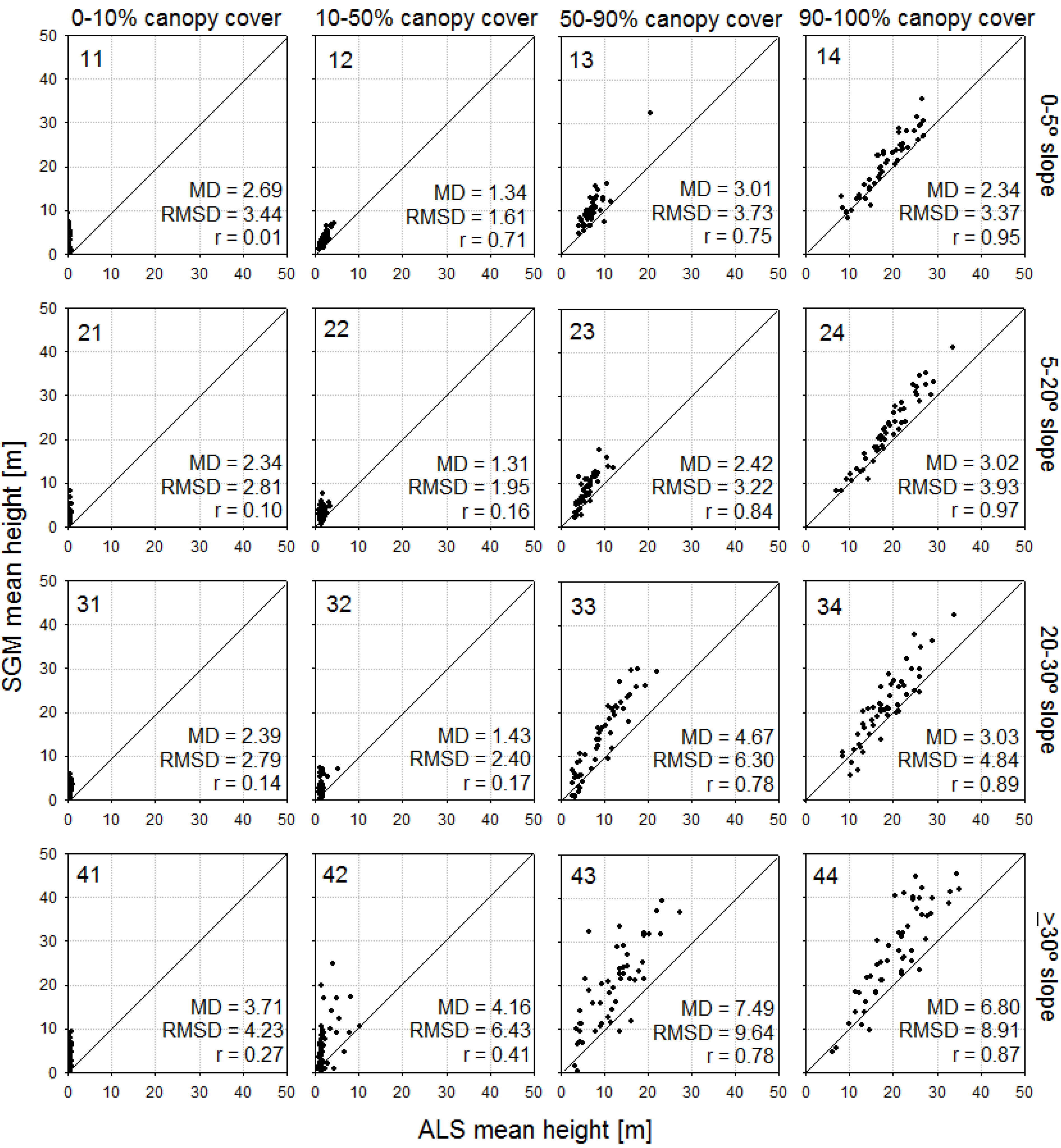
For mean height (Hmean), MDs across all strata are generally larger than for P90 (mean MD for Hmean = 3.26 m), whereas the averaged RMSD of 4.36 m is almost equal to that of the P90. Examining the different canopy cover classes (Figure 6) indicates that strong correlations (i.e., |r| ≥ 0.8) between ALS and SGM Hmean occur for canopy cover ≥50%. The average MD for Hmean is 4.38 m for canopy cover 50%–90% and 3.79 m for strata with canopy cover 90%–100%. The corresponding RMSDs are 5.72 m and 5.26 m, respectively. Examining only those strata with canopy cover ≥50%, the scatterplots in Figure 6 reveal a decreasing correspondence between the SGM and ALS Hmean with increasing slope. This is particularly evident at slopes ≥30°, with MD and RMSD of 7.15 m and 9.28 m (mean of strata 43 and 44), respectively, compared to 3.08 m and 4.23 m for the less steep strata (mean of strata 13, 14, 23, 24, 33, 34). The differences between SGM and ALS Hmean metric medians were significant across all strata (Table 8).

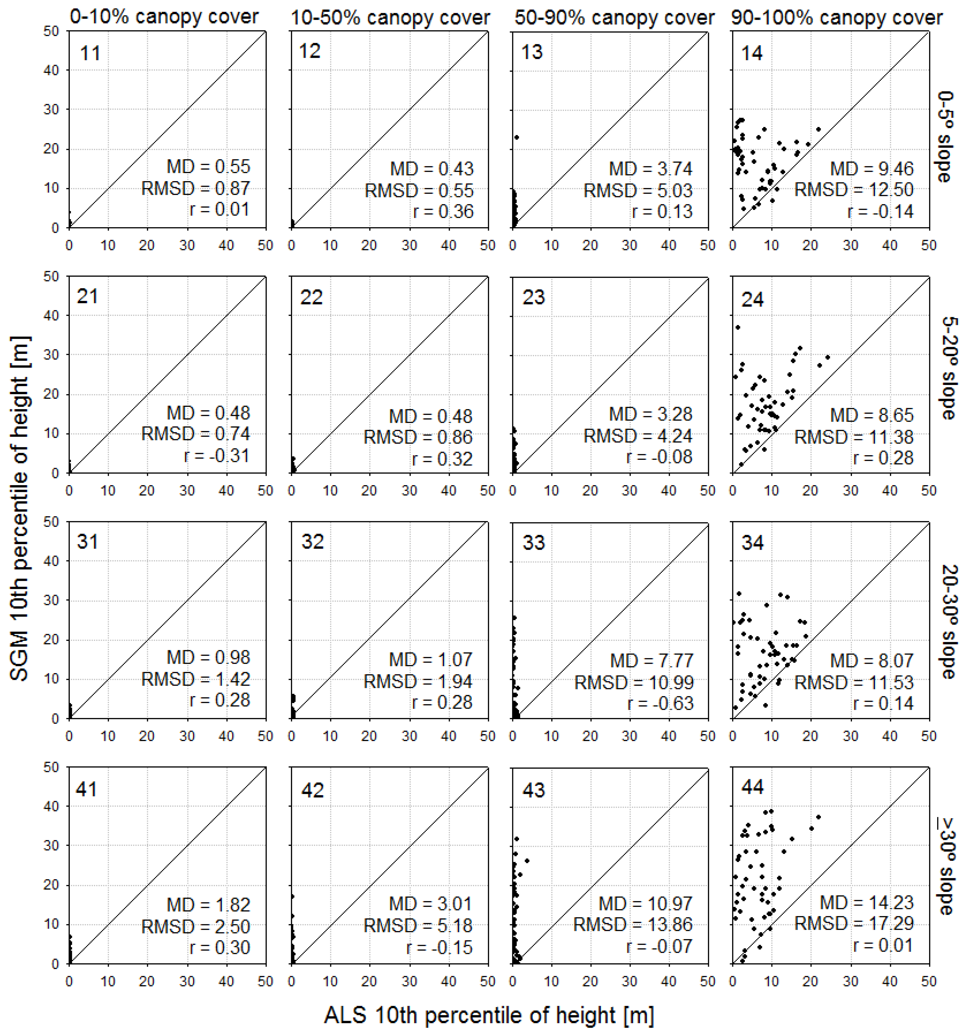
When examining the 10th percentile of heights (P10), it is evident that there is greater disparity between SGM and ALS metric values. Of note, MD and RMSD are very large for P10, particularly for high canopy cover and steep slopes (Figure 7), and SGM and ALS median metric values are significantly different for all strata (Table 8). Trends for other metrics vary. The coefficient of variation of point heights (CoV) is consistently smaller for SGM data across all strata (i.e., MD is always negative), indicative of the different canopy penetration capacity of the SGM relative to the ALS data. Values for the SGM skewness metric are likewise smaller than their ALS counterparts, except for strata with canopy cover >90% (i.e., 14, 24, 34, 44). SGM kurtosis values tend to be lower than their ALS counterparts, except for strata with 50%–90% canopy cover.

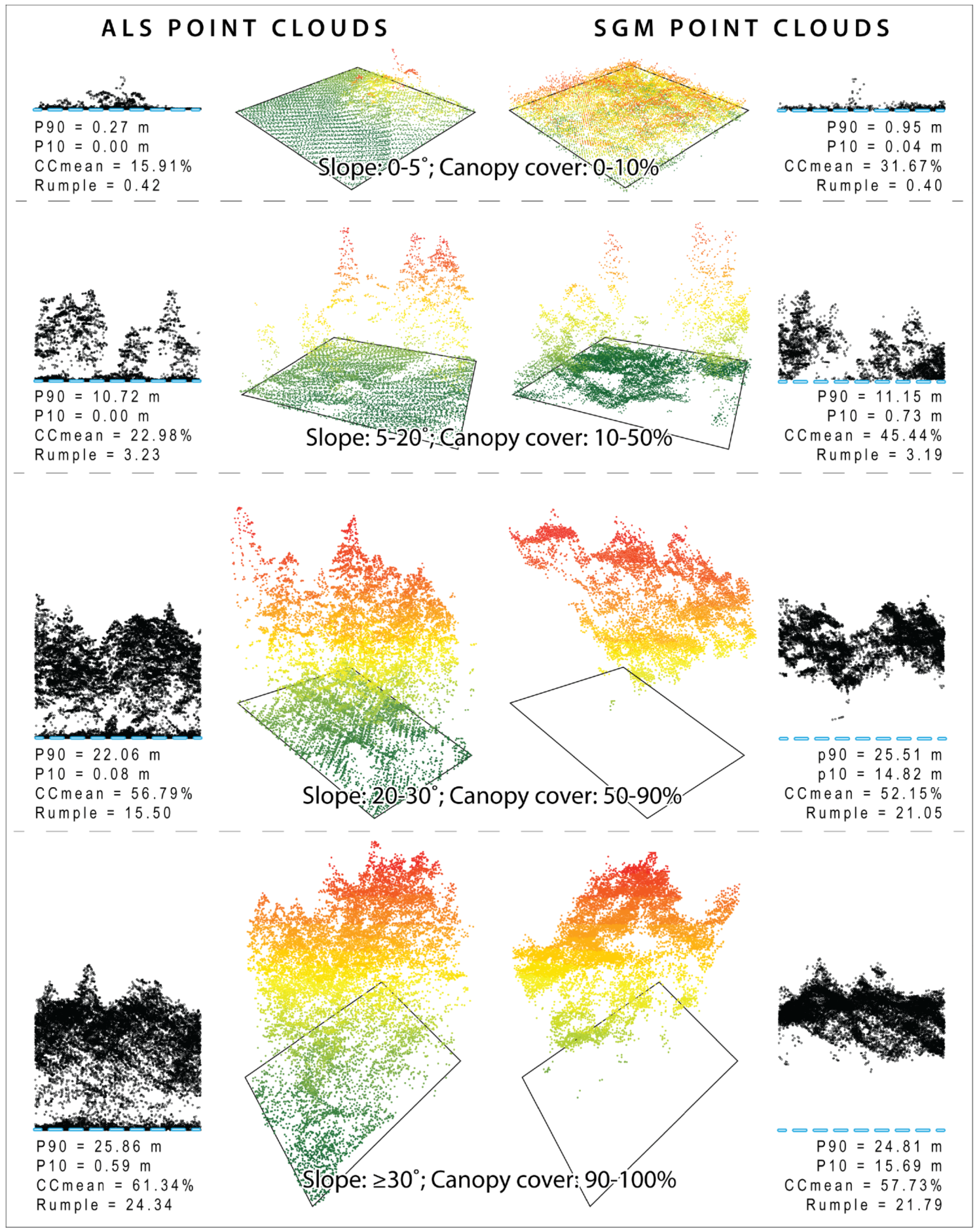
Figure 4. Selected comparison of ALS and SGM point clouds for the same cell locations across the range of slope and canopy cover conditions, as described in Table 5. Metrics P90, P10, CCmean, and Rumple are defined in Table 6.

Figure 4. Selected comparison of ALS and SGM point clouds for the same cell locations across the range of slope and canopy cover conditions, as described in Table 5. Metrics P90, P10, CCmean, and Rumple are defined in Table 6.

Table 7. Results of metric comparisons across strata defined in Table 5. Mean Difference (MD) and Root Mean Squared Difference (RMSD) are calculated using Equations (1) and (2), respectively. Spearman rank order correlations (r) are reported between ALS and SGM metrics. Values in italics are significant at p < 0.05. Metrics are defined in Table 6.

	Hmean			CoV			Skewness			Kurtosis
STRATUM	MD	RMSD	r	MD	RMSD	r	MD	RMSD	R	MD	RMSD	r
11	2.69	3.44	0.01	−0.07	0.50	0.21	−0.89	2.20	0.00	−6.89	19.47	−0.16
12	1.34	1.61	0.71	−0.62	0.69	0.04	−0.91	1.10	0.17	−2.38	3.98	0.08
13	3.01	3.73	0.75	−0.40	0.41	0.64	−0.45	0.58	0.60	0.34	1.20	0.05
14	2.34	3.37	0.95	−0.20	0.24	0.00	1.25	1.42	0.36	−1.03	2.85	0.09
21	2.34	2.81	0.10	−0.12	0.34	−0.35	−0.80	1.81	−0.26	−3.52	11.83	−0.19
22	1.31	1.95	0.16	−0.27	0.43	0.32	−0.36	1.00	0.30	0.00	4.98	0.37
23	2.42	3.22	0.84	−0.36	0.40	0.28	−0.28	0.60	0.31	0.69	1.49	−0.14
24	3.02	3.93	0.97	−0.19	0.21	0.36	1.03	1.30	0.11	−1.14	2.62	0.18
31	2.39	2.79	0.14	−0.21	0.39	0.14	−1.43	3.88	0.09	−21.36	123.72	0.01
32	1.43	2.40	0.17	−0.18	0.41	0.38	−0.48	1.18	0.29	−0.14	6.60	0.15
33	4.67	6.30	0.93	−0.27	0.42	0.17	−0.16	0.62	0.51	0.64	1.47	−0.08
34	3.03	4.84	0.89	−0.18	0.22	−0.03	1.09	1.30	0.13	−1.30	2.44	0.04
41	3.71	4.32	0.27	−0.24	0.34	0.05	−1.25	1.69	0.15	−6.89	17.60	0.14
42	4.16	6.50	0.41	−0.47	0.79	−0.03	−1.01	1.51	0.19	−3.88	13.48	0.22
43	7.49	9.64	0.78	−0.37	0.45	0.04	−0.24	0.66	0.29	0.47	2.66	0.29
44	6.80	8.91	0.87	−0.23	0.29	0.15	0.52	0.80	0.34	−0.23	0.99	0.37
Mean	3.26	4.36	0.56	−0.27	0.41	0.15	−0.27	1.35	0.22	−2.91	13.59	0.09
	P10			P90			CCmean			Rumple
STRATUM	MD	RMSD	r	MD	RMSD	r	MD	RMSD	r	MD	RMSD	r
11	0.55	0.87	0.01	5.09	6.40	0.00	22.83	29.04	0.10	−4.89	37.18	−0.20
12	0.43	0.55	0.36	0.63	1.76	0.68	15.28	17.06	0.01	−0.67	0.99	0.70
13	3.74	5.03	0.13	0.13	2.67	0.75	5.15	6.75	0.47	−0.92	1.37	−0.06
14	9.46	12.50	−0.14	−0.27	2.14	0.96	−12.20	14.71	−0.02	−0.26	0.89	0.59
21	0.48	0.74	−0.31	4.61	5.55	0.21	9.54	14.97	−0.37	5.24	20.01	0.14
22	0.48	0.86	0.32	1.63	3.27	0.08	8.82	12.99	0.12	0.20	0.89	0.16
23	3.28	4.24	−0.08	0.09	1.96	0.90	4.98	7.21	0.27	−0.94	1.26	0.54
24	8.65	11.38	0.28	0.04	1.91	0.98	−7.30	9.39	0.15	−0.57	0.96	0.56
31	0.98	1.42	0.28	4.01	4.73	0.12	10.17	13.88	−0.01	2.85	14.17	−0.04
32	1.07	1.94	0.28	1.15	3.95	0.12	6.35	10.18	0.32	1.86	14.07	0.33
33	7.77	10.99	−0.63	1.46	3.58	0.95	2.46	8.05	0.35	−1.42	1.97	0.67
34	8.07	11.53	0.14	0.60	3.27	0.92	−8.26	10.53	0.03	−0.32	1.09	0.48
41	1.82	2.50	0.30	5.83	6.66	0.20	11.57	14.62	−0.08	3.33	14.53	0.08
42	3.01	5.18	−0.15	4.65	9.70	0.45	11.97	17.28	0.09	3.91	19.53	0.50
43	10.97	13.86	−0.07	3.43	6.91	0.83	3.63	8.62	0.15	−1.51	2.19	0.32
44	14.23	17.29	0.01	2.29	5.55	0.89	−5.56	8.49	0.32	−0.90	1.73	0.54
Mean	4.69	6.30	0.05	2.21	4.37	0.56	4.96	12.73	0.12	0.31	8.30	0.33

Table 7. Results of metric comparisons across strata defined in Table 5. Mean Difference (MD) and Root Mean Squared Difference (RMSD) are calculated using Equations (1) and (2), respectively. Spearman rank order correlations (r) are reported between ALS and SGM metrics. Values in italics are significant at p < 0.05. Metrics are defined in Table 6.

	Hmean			CoV			Skewness			Kurtosis
STRATUM	MD	RMSD	r	MD	RMSD	r	MD	RMSD	R	MD	RMSD	r
11	2.69	3.44	0.01	−0.07	0.50	0.21	−0.89	2.20	0.00	−6.89	19.47	−0.16
12	1.34	1.61	0.71	−0.62	0.69	0.04	−0.91	1.10	0.17	−2.38	3.98	0.08
13	3.01	3.73	0.75	−0.40	0.41	0.64	−0.45	0.58	0.60	0.34	1.20	0.05
14	2.34	3.37	0.95	−0.20	0.24	0.00	1.25	1.42	0.36	−1.03	2.85	0.09
21	2.34	2.81	0.10	−0.12	0.34	−0.35	−0.80	1.81	−0.26	−3.52	11.83	−0.19
22	1.31	1.95	0.16	−0.27	0.43	0.32	−0.36	1.00	0.30	0.00	4.98	0.37
23	2.42	3.22	0.84	−0.36	0.40	0.28	−0.28	0.60	0.31	0.69	1.49	−0.14
24	3.02	3.93	0.97	−0.19	0.21	0.36	1.03	1.30	0.11	−1.14	2.62	0.18
31	2.39	2.79	0.14	−0.21	0.39	0.14	−1.43	3.88	0.09	−21.36	123.72	0.01
32	1.43	2.40	0.17	−0.18	0.41	0.38	−0.48	1.18	0.29	−0.14	6.60	0.15
33	4.67	6.30	0.93	−0.27	0.42	0.17	−0.16	0.62	0.51	0.64	1.47	−0.08
34	3.03	4.84	0.89	−0.18	0.22	−0.03	1.09	1.30	0.13	−1.30	2.44	0.04
41	3.71	4.32	0.27	−0.24	0.34	0.05	−1.25	1.69	0.15	−6.89	17.60	0.14
42	4.16	6.50	0.41	−0.47	0.79	−0.03	−1.01	1.51	0.19	−3.88	13.48	0.22
43	7.49	9.64	0.78	−0.37	0.45	0.04	−0.24	0.66	0.29	0.47	2.66	0.29
44	6.80	8.91	0.87	−0.23	0.29	0.15	0.52	0.80	0.34	−0.23	0.99	0.37
Mean	3.26	4.36	0.56	−0.27	0.41	0.15	−0.27	1.35	0.22	−2.91	13.59	0.09
	P10			P90			CCmean			Rumple
STRATUM	MD	RMSD	r	MD	RMSD	r	MD	RMSD	r	MD	RMSD	r
11	0.55	0.87	0.01	5.09	6.40	0.00	22.83	29.04	0.10	−4.89	37.18	−0.20
12	0.43	0.55	0.36	0.63	1.76	0.68	15.28	17.06	0.01	−0.67	0.99	0.70
13	3.74	5.03	0.13	0.13	2.67	0.75	5.15	6.75	0.47	−0.92	1.37	−0.06
14	9.46	12.50	−0.14	−0.27	2.14	0.96	−12.20	14.71	−0.02	−0.26	0.89	0.59
21	0.48	0.74	−0.31	4.61	5.55	0.21	9.54	14.97	−0.37	5.24	20.01	0.14
22	0.48	0.86	0.32	1.63	3.27	0.08	8.82	12.99	0.12	0.20	0.89	0.16
23	3.28	4.24	−0.08	0.09	1.96	0.90	4.98	7.21	0.27	−0.94	1.26	0.54
24	8.65	11.38	0.28	0.04	1.91	0.98	−7.30	9.39	0.15	−0.57	0.96	0.56
31	0.98	1.42	0.28	4.01	4.73	0.12	10.17	13.88	−0.01	2.85	14.17	−0.04
32	1.07	1.94	0.28	1.15	3.95	0.12	6.35	10.18	0.32	1.86	14.07	0.33
33	7.77	10.99	−0.63	1.46	3.58	0.95	2.46	8.05	0.35	−1.42	1.97	0.67
34	8.07	11.53	0.14	0.60	3.27	0.92	−8.26	10.53	0.03	−0.32	1.09	0.48
41	1.82	2.50	0.30	5.83	6.66	0.20	11.57	14.62	−0.08	3.33	14.53	0.08
42	3.01	5.18	−0.15	4.65	9.70	0.45	11.97	17.28	0.09	3.91	19.53	0.50
43	10.97	13.86	−0.07	3.43	6.91	0.83	3.63	8.62	0.15	−1.51	2.19	0.32
44	14.23	17.29	0.01	2.29	5.55	0.89	−5.56	8.49	0.32	−0.90	1.73	0.54
Mean	4.69	6.30	0.05	2.21	4.37	0.56	4.96	12.73	0.12	0.31	8.30	0.33

Figure 5. Scatterplots of ALS and SGM 90th percentiles of height (P90) metrics across the strata defined by slope and canopy cover classes.

Figure 5. Scatterplots of ALS and SGM 90th percentiles of height (P90) metrics across the strata defined by slope and canopy cover classes.

Table 8. Results of Wilcoxon matched pairs test for statistical significance of the differences between the metric medians from SGM and ALS point cloud data at p < 0.05.

Metric	Number of Strata with No Significant Differences	Stratum with No Significant Difference
Hmean	0
CoV	1	11
Skewness	0
Kurtosis	0
P10	0
P90	5	13, 14, 23, 24, 34
CCmean	0
Rumple	2	22, 42

Table 8. Results of Wilcoxon matched pairs test for statistical significance of the differences between the metric medians from SGM and ALS point cloud data at p < 0.05.

Metric	Number of Strata with No Significant Differences	Stratum with No Significant Difference
Hmean	0
CoV	1	11
Skewness	0
Kurtosis	0
P10	0
P90	5	13, 14, 23, 24, 34
CCmean	0
Rumple	2	22, 42

Figure 6. Scatterplots of ALS and SGM mean height (Hmean) metrics across the strata defined by slope and canopy cover classes.

Figure 6. Scatterplots of ALS and SGM mean height (Hmean) metrics across the strata defined by slope and canopy cover classes.

Figure 7. Scatterplots of ALS and SGM 10th percentiles of height (P10) across the strata defined by slope and canopy cover classes.

Figure 7. Scatterplots of ALS and SGM 10th percentiles of height (P10) across the strata defined by slope and canopy cover classes.

For the canopy cover metric (CCmean, the proportion of point heights greater than the mean point height), the r values are generally low, indicating that there is not a strong correlation between the SGM and ALS CCmean. The MD generally decreased with increasing canopy cover, except for strata with canopy cover >90%. CCmean_SGM overestimates canopy cover relative to CCmean_ALS by an average of 13.53% for strata with canopy cover of 0%–10%, and conversely, CCmean_SGM underestimates cover relative to CCmean_ALS by an average of 8.33% for strata with canopy cover of 90%–100% (Table 7). The RMSD values are lowest for strata with canopy cover of 50%–90% (mean = 7.66%), and increase both for higher and lower canopy cover. Examining the different slope scenarios, no consistent pattern in CCmean was found.

For Rumple, a measure of the canopy surface roughness, the MD values indicate that the SGM Rumple metric values are greater than ALS counterparts for low cover scenarios (except for slopes 0°–5°), and lower than ALS for high cover scenarios. The high RMSD values for the low cover strata (mean RMSD = 21.47 for canopy cover 0%–10%) in conjunction with the correlation being almost zero (mean r = 0.02 for canopy cover 0%–10%) point to the great discrepancy for Rumple at low canopy cover (Table 7). For the densely covered samples (canopy cover 90%–100%), the RMSD = 1.17 on average and r = 0.54, indicating a higher level of correspondence for the SGM and ALS based canopy surface at high canopy covers.

Correlations between the input metrics used for model development and the plot-based estimates of H, G, and V are summarized in Table 9. For the ALS data, the metrics that were most strongly correlated with Lorey’s mean height were P90 (r = 0.96), Hmean (r = 0.88) and Rumple (r = 0.76). For the SGM data, Hmean (r = 0.91) and P90 (r = 0.90) had the strongest correlation with Lorey’s mean height (Figure 8). Of note, P10_SGM—which was an average of 14.33 m greater than P10_ALS for the plot data (n = 140)—was also strongly correlated with Lorey’s mean height (r = 0.88), in contrast to P10_ALS (r = 0.18). Recall that for the sample cells, which covered a much broader range of forest conditions and included canopy cover <50%, P10_SGM and P10_ALS differed by an average of 4.69 m (Table 7). Hmean_SGM was on average 5.73 m greater than Hmean_ALS (compared to 3.26 m greater for the sample cells), and P90_SGM was an average of 0.96 m greater than P90_ALS (compared to 2.21 m greater for the ground plots). This further underscores some of the important differences in how ALS and SGM data characterize the vertical canopy profile. The most strongly correlated metrics with basal area for both ALS and SGM were P90 (r = 0.55 and 0.52, respectively) and Hmean (r = 0.50 and 0.51, respectively). For gross volume, ALS-derived P90 had the strongest correlation (r = 0.80), followed by Hmean (r = 0.75) and Rumple (r = 0.65). In contrast, P90_SGM P90 and Hmean had the strongest correlations with gross volume (r = 0.76), closely followed by P10 (r = 0.74).

Table 9. Spearman rank order correlation coefficients (r) between point cloud metrics and plot-based estimates of H, G, and V for the plot data (n = 140). Values in italics are significant at p < 0.05.

Metric	H		G		V
	ALS	SGM	ALS	SGM	ALS	SGM
Hmean	0.88	0.91	0.50	0.51	0.75	0.76
CoV	−0.07	−0.59	0.08	−0.31	−0.04	−0.49
Skewness	−0.15	0.12	−0.08	0.08	−0.18	0.10
Kurtosis	0.02	0.05	−0.11	−0.07	0.00	−0.01
P10	0.24	0.88	−0.02	0.49	0.12	0.74
P90	0.96	0.90	0.55	0.52	0.80	0.76
CCmean	0.19	−0.16	0.15	−0.07	0.23	−0.11
Rumple	0.76	0.46	0.54	0.40	0.65	0.45

Table 9. Spearman rank order correlation coefficients (r) between point cloud metrics and plot-based estimates of H, G, and V for the plot data (n = 140). Values in italics are significant at p < 0.05.

Metric	H		G		V
	ALS	SGM	ALS	SGM	ALS	SGM
Hmean	0.88	0.91	0.50	0.51	0.75	0.76
CoV	−0.07	−0.59	0.08	−0.31	−0.04	−0.49
Skewness	−0.15	0.12	−0.08	0.08	−0.18	0.10
Kurtosis	0.02	0.05	−0.11	−0.07	0.00	−0.01
P10	0.24	0.88	−0.02	0.49	0.12	0.74
P90	0.96	0.90	0.55	0.52	0.80	0.76
CCmean	0.19	−0.16	0.15	−0.07	0.23	−0.11
Rumple	0.76	0.46	0.54	0.40	0.65	0.45

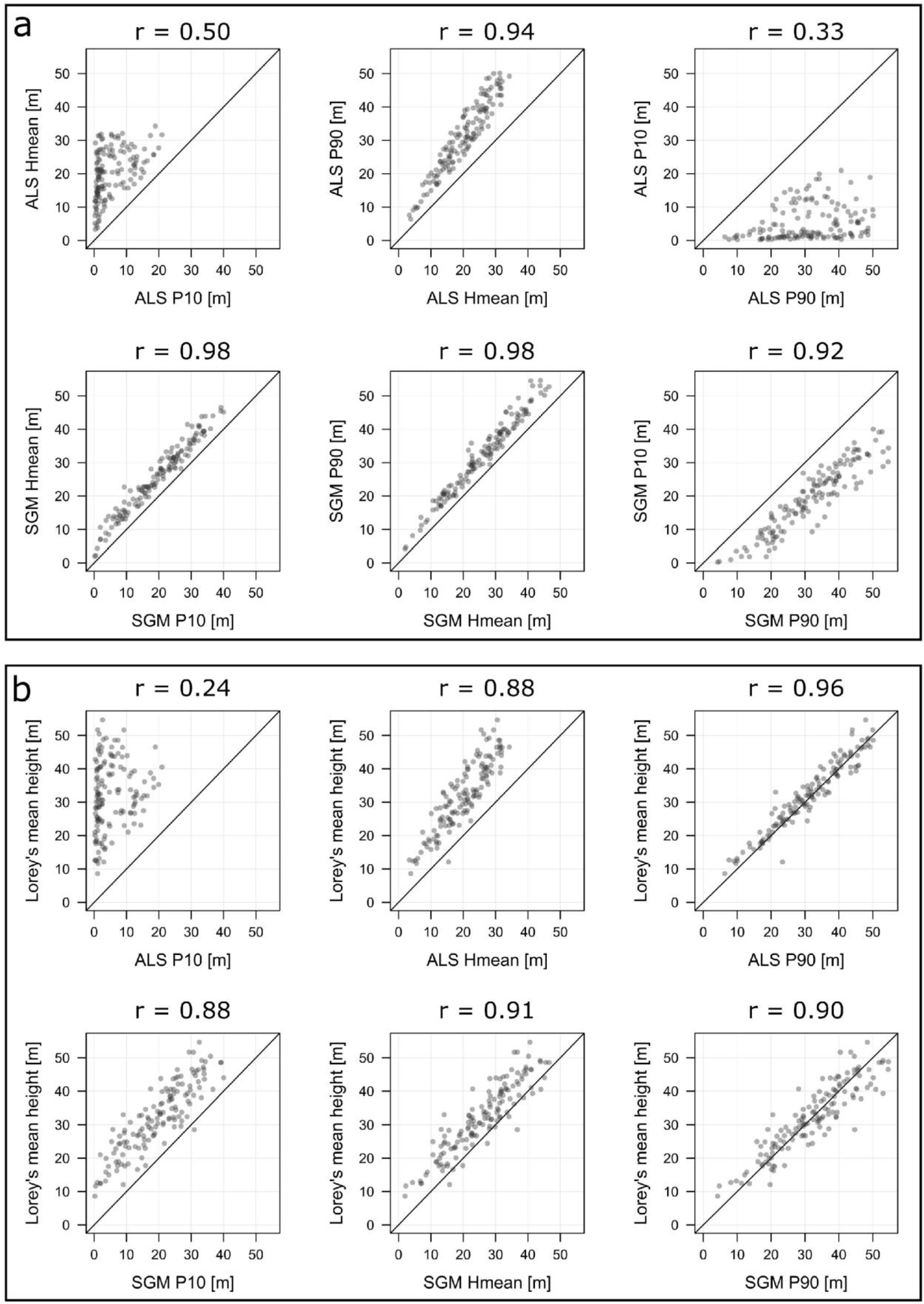
Figure 8. Relationships between the three height metrics P90, Hmean, and P10 (Table 6) for ALS and SGM data relative to one another (a) and relative to plot estimates of Lorey’s mean height (b). Spearman rank-order correlations (r) are provided.

Figure 8. Relationships between the three height metrics P90, Hmean, and P10 (Table 6) for ALS and SGM data relative to one another (a) and relative to plot estimates of Lorey’s mean height (b). Spearman rank-order correlations (r) are provided.

We further explored the relationships between P90, Hmean, and P10 for ALS and SGM, both relative to one another and to the ground plot estimates of Lorey’s mean height (Figure 8) using Spearman’s rank order correlation. Whereas P10_ALS is weakly correlated with P90_ALS (r = 0.33) and Hmean_ALS (r = 0.50), P10_SGM is very strongly correlated with P90_SGM (r = 0.98) and Hmean_SGM (r = 0.98). Moreover, P10_SGM is strongly correlated with ground plot estimates of Lorey’s mean height (r = 0.88), whereas P10_ALS is not (r = 0.24) (Table 9).

3.2. Forest Attribute Modelling

We generated individual RF models for H, G, and V using point cloud metrics generated from ALS and SGM data (Table 6). Overall, both data sources resulted in models with similar relationships between predicted and observed values (Table 10) and these results are in keeping with those reported in other studies (e.g., Table 1). The difference between RMSE% for H_ALS and H_SGM was the largest among attributes considered, with H_SGM RMSE% being 5.04% larger (RMSE = 1.61 m larger) than H_ALS. 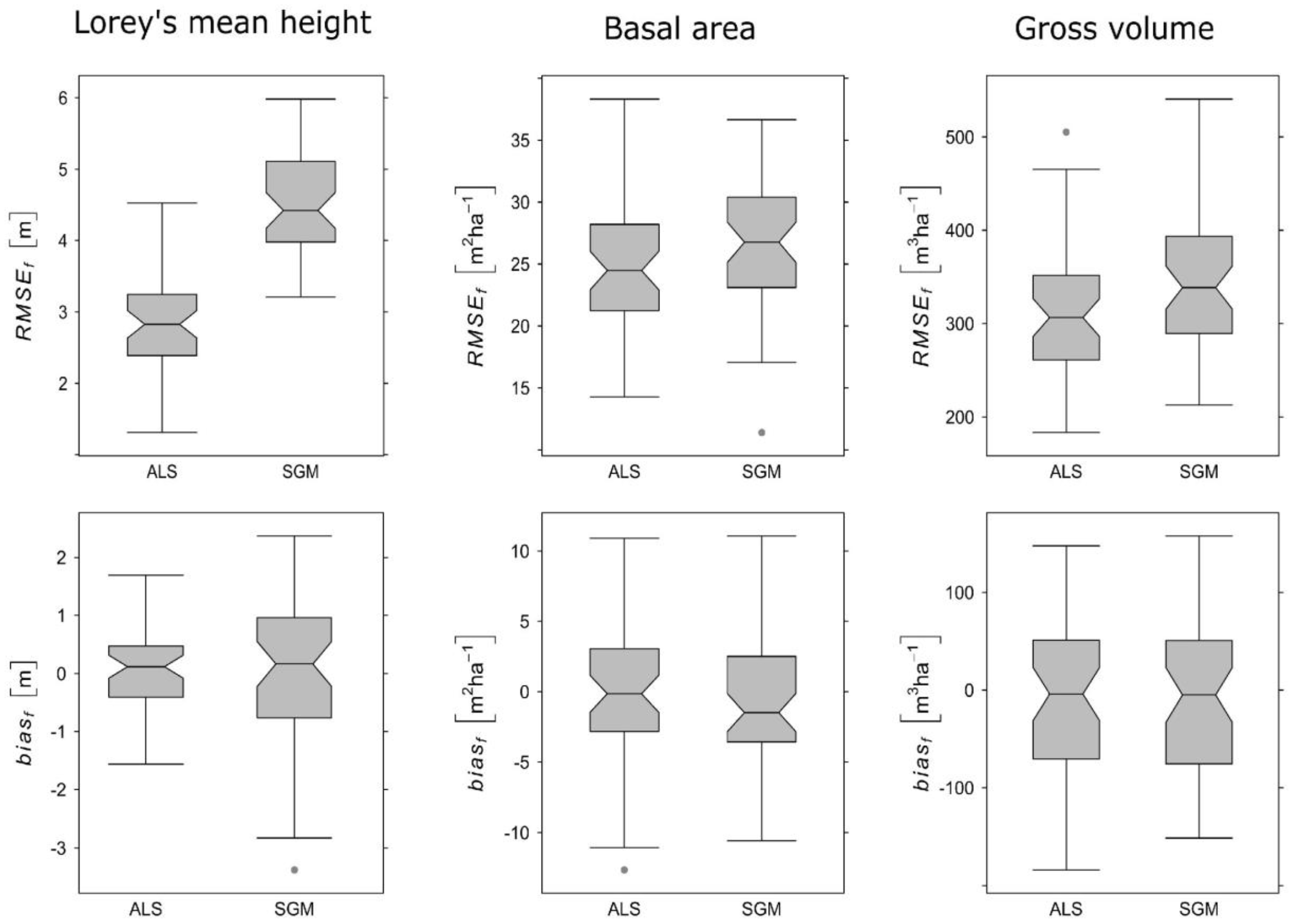Bias was positive and small for both H_ALS and H_SGM, differing by 0.1%. RMSE for G_ALS and G_SGM differed by only 2.3% (1.63 m²·ha⁻¹) (Figure 9). Bias was negative for both G_ALS and G_SGM, differing by 0.67%. The RMSE% for V_SGM was 3.63% greater than V_ALS, and the bias differed by 0.16%. 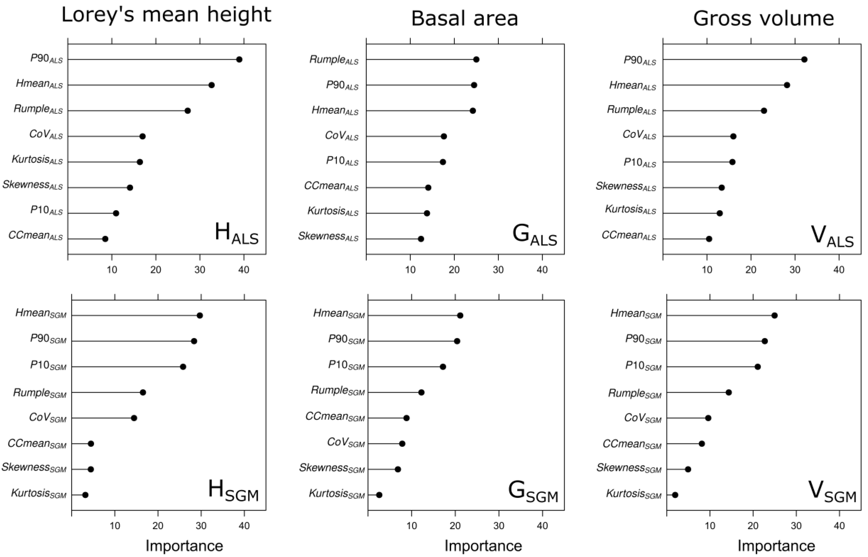Figure 10 summarizes the variable importance metrics for model predictors. For ALS models, P90, Hmean, and Rumple were consistently the top three predictors for models for H, G, and V. For the SGM models, Hmean, P90, and P10 were consistently the top three predictors in terms of variable importance.

Table 10. Absolute and relative RMSE and bias from 10-fold cross validation (repeated five times) for ALS and SGM models of Loreys’ mean height (H), basal area (G), and gross volume (V).

Attribute	Mean (Observed)	RMSE	RMSE%	bias	bias%
HALS (m)	32.10	2.88	8.96	0.05	0.16
HSGM (m)	32.10	4.49	14.00	0.02	0.06
GALS (m2·ha−1)	70.74	25.02	35.38	−0.38	−0.54
GSGM (m2·ha−1)	70.74	26.65	37.68	−0.86	−1.21
VALS (m3·ha−1)	939.86	312.42	33.24	−6.74	−0.72
VSGM (m3·ha−1)	939.86	346.55	36.87	−8.31	−0.88

Table 10. Absolute and relative RMSE and bias from 10-fold cross validation (repeated five times) for ALS and SGM models of Loreys’ mean height (H), basal area (G), and gross volume (V).

Attribute	Mean (Observed)	RMSE	RMSE%	bias	bias%
HALS (m)	32.10	2.88	8.96	0.05	0.16
HSGM (m)	32.10	4.49	14.00	0.02	0.06
GALS (m2·ha−1)	70.74	25.02	35.38	−0.38	−0.54
GSGM (m2·ha−1)	70.74	26.65	37.68	−0.86	−1.21
VALS (m3·ha−1)	939.86	312.42	33.24	−6.74	−0.72
VSGM (m3·ha−1)	939.86	346.55	36.87	−8.31	−0.88

Figure 9. Distribution of absolute RMSE_f and bias_f values as obtained from the 10-fold cross validation (repeated five times). RMSE_f and bias_f are calculated using Equations (3) and (4). Boxplots are shown for the Random Forests (RF) models of Lorey’s mean height, basal area, and gross volume based on ALS and SGM derived predictor variables.

Figure 9. Distribution of absolute RMSE_f and bias_f values as obtained from the 10-fold cross validation (repeated five times). RMSE_f and bias_f are calculated using Equations (3) and (4). Boxplots are shown for the Random Forests (RF) models of Lorey’s mean height, basal area, and gross volume based on ALS and SGM derived predictor variables.

Figure 10. Variable importance measures generated for each of the Random Forests models.

Figure 10. Variable importance measures generated for each of the Random Forests models.

In order to relate the differences observed between the ALS and SGM metrics across the slope and canopy cover strata to the model outcomes, we calculated relative RMSE and bias, by stratum for each of the strata having sufficient samples (Table 11). This limits our comparison to strata that had ≥50% canopy cover. In general, the results by strata are similar to the overall results: SGM models have larger RMSE and bias relative to ALS models, but differences are generally small and not statistically significant. Specifically, differences in bias for H, G, and V were not found to be statistically significant, with the exception of bias in G for stratum 23. Differences in RMSE were significant for H for strata 24, 34 and 44, and for strata 44 for G and V. Overall, bias and RMSE did not vary with slope; however, the greatest difference in RMSE and bias between ALS and SGM model outcomes typically occurred for stratum 33 (slope 0°–30°; cover 50%–90%) and stratum 44 (slope ≥ 30°; cover 90%–100%).

Table 11. Summary of relative bias and RMSE, by strata defined according to slope and canopy cover criteria. The number of plots for each stratum is provided in parentheses. p-values of a paired t-test are reported (those marked with a * are significant, p < 0.05).

Lorey’s Mean Height (m)
	HALS	HSGM	HALS − HSGM	p	HALS	HSGM	HALS − HSGM	p
Stratum	RMSE%	RMSE%	ΔRMSE%		bias%	bias%	Δbias%
14 (12)	13.59	14.04	−0.45	0.85	−3.1	−5.51	2.41	0.45
23 (14)	7.36	8.34	−0.98	0.39	0.36	0.82	−0.46	0.68
24 (37)	8.60	14.09	−5.49	0.00*	3.83	3.85	−0.02	0.99
33 (5)	12.76	20.66	−7.90	0.15	2.77	8.94	−6.17	0.47
34 (32)	6.06	12.96	−6.90	0.00*	−0.78	−0.35	−0.43	0.82
43 (9)	10.18	11.81	−1.63	0.51	−0.04	0.94	−0.98	0.77
44 (28)	10.06	17.74	−7.68	0.02*	−2.88	−4.58	1.70	0.55
Basal Area (m2·ha−1)
	GALS	GSGM	GALS − GSGM	p	GALS	GSGM	GALS − GSGM	p
Stratum	RMSE%	RMSE%	ΔRMSE%		bias%	bias%	Δbias%
14 (12)	37.06	33.66	3.4	0.69	−18.26	−22.24	3.98	0.65
23 (14)	18.58	25.12	−6.54	0.10	2.41	10.06	−7.65	0.04*
24 (37)	34.42	37.64	−3.22	0.13	−1.72	−1.65	−0.07	0.98
33 (5)	63.49	61.72	1.77	0.86	40.19	50.73	−10.54	0.39
34 (32)	30.05	28.01	2.04	0.58	3.09	−3.14	6.23	0.09
43 (9)	41.04	42.57	−1.53	0.72	−15.9	−11.45	−4.45	0.40
44 (28)	44.07	50.91	−6.84	0.02*	0.57	−2.78	3.35	0.43
Gross Volume (m3·ha−1)
	VALS	VSGM	VALS − VSGM	p	VALS	VSGM	VALS − VSGM	p
Stratum	RMSE%	RMSE%	ΔRMSE%		bias%	bias%	Δbias%
14 (12)	35.31	32.52	2.79	0.64	−10.4	−13.38	2.98	0.68
23 (14)	15.49	17.28	−1.79	0.47	1.57	5.07	−3.51	0.23
24 (37)	36.26	40.18	−3.92	0.06	4.80	5.60	−0.80	0.80
33 (5)	48.27	47.99	0.28	0.97	28.29	39.96	−11.67	0.35
34 (32)	31.17	28.91	2.26	0.51	−0.05	−3.47	3.42	0.40
43 (9)	36.69	31.96	4.73	0.37	−8.89	−6.49	−2.40	0.69
44 (28)	40.08	51.43	−11.35	0.02*	−6.06	−9.16	3.10	0.53

Table 11. Summary of relative bias and RMSE, by strata defined according to slope and canopy cover criteria. The number of plots for each stratum is provided in parentheses. p-values of a paired t-test are reported (those marked with a * are significant, p < 0.05).

Lorey’s Mean Height (m)
	HALS	HSGM	HALS − HSGM	p	HALS	HSGM	HALS − HSGM	p
Stratum	RMSE%	RMSE%	ΔRMSE%		bias%	bias%	Δbias%
14 (12)	13.59	14.04	−0.45	0.85	−3.1	−5.51	2.41	0.45
23 (14)	7.36	8.34	−0.98	0.39	0.36	0.82	−0.46	0.68
24 (37)	8.60	14.09	−5.49	0.00*	3.83	3.85	−0.02	0.99
33 (5)	12.76	20.66	−7.90	0.15	2.77	8.94	−6.17	0.47
34 (32)	6.06	12.96	−6.90	0.00*	−0.78	−0.35	−0.43	0.82
43 (9)	10.18	11.81	−1.63	0.51	−0.04	0.94	−0.98	0.77
44 (28)	10.06	17.74	−7.68	0.02*	−2.88	−4.58	1.70	0.55
Basal Area (m2·ha−1)
	GALS	GSGM	GALS − GSGM	p	GALS	GSGM	GALS − GSGM	p
Stratum	RMSE%	RMSE%	ΔRMSE%		bias%	bias%	Δbias%
14 (12)	37.06	33.66	3.4	0.69	−18.26	−22.24	3.98	0.65
23 (14)	18.58	25.12	−6.54	0.10	2.41	10.06	−7.65	0.04*
24 (37)	34.42	37.64	−3.22	0.13	−1.72	−1.65	−0.07	0.98
33 (5)	63.49	61.72	1.77	0.86	40.19	50.73	−10.54	0.39
34 (32)	30.05	28.01	2.04	0.58	3.09	−3.14	6.23	0.09
43 (9)	41.04	42.57	−1.53	0.72	−15.9	−11.45	−4.45	0.40
44 (28)	44.07	50.91	−6.84	0.02*	0.57	−2.78	3.35	0.43
Gross Volume (m3·ha−1)
	VALS	VSGM	VALS − VSGM	p	VALS	VSGM	VALS − VSGM	p
Stratum	RMSE%	RMSE%	ΔRMSE%		bias%	bias%	Δbias%
14 (12)	35.31	32.52	2.79	0.64	−10.4	−13.38	2.98	0.68
23 (14)	15.49	17.28	−1.79	0.47	1.57	5.07	−3.51	0.23
24 (37)	36.26	40.18	−3.92	0.06	4.80	5.60	−0.80	0.80
33 (5)	48.27	47.99	0.28	0.97	28.29	39.96	−11.67	0.35
34 (32)	31.17	28.91	2.26	0.51	−0.05	−3.47	3.42	0.40
43 (9)	36.69	31.96	4.73	0.37	−8.89	−6.49	−2.40	0.69
44 (28)	40.08	51.43	−11.35	0.02*	−6.06	−9.16	3.10	0.53

It is useful to relate the stratum-specific model performance back to our exploration of metrics and their variability across our slope and cover strata. In this context, recall that the top three predictors for the ALS models were P90, Hmean, and Rumple, and for the SGM models, the top predictors were Hmean, P90, and P10. The greatest difference between H_ALS and H_SGM was for stratum 33 (slope 20°–30°; cover 50%–90%), where RMSE was 7.89% greater and bias was 6.17% greater for H_SGM. Correlations for P90 and Hmean were high for stratum 33 (0.95 and 0.93, respectively), but correlation was negative for P10 (−0.63). For G, the greatest difference between G_ALS and G_SGM was for stratum 23 (slope = 5°–20°; cover = 50%–90%). G_SGM RMSE was 6.54% greater and bias was 7.65% greater when compared to the G_ALS model.

Gobakken et al. [19] indicate that large-area operational scale implementation of DAP for an area-based approach may be difficult when imagery is acquired under different conditions (i.e., on different dates with different illumination conditions). In our study area, we were in a unique position to test the impact of different acquisition dates on SGM model outcomes. Table 12 summarizes the relative RMSE for H, G, and V, by image acquisition date. Overall, there was no consistent trend in model error as a result of varying image acquisition conditions, specifically, differences in solar elevation. Generally, bias and RMSE were greater for SGM, but not markedly greater, with the only statistically significant differences in RMSE for the 16 August 2012 date, for both H and G, and the 4 October 2012 date for H. The greatest difference in relative RMSE between ALS and SGM came on 16 August 2012 for H and 25 September 2012 for G and V.

Table 12. Summary of relative bias and RMSE for H, G, and V, by image acquisition date. The number of corresponding field plots is provided in parentheses. p-values of a paired t-test are reported (those marked with a * are significant, p < 0.05).

	Lorey’s Mean Height (m)
	HALS	HSGM	HALS − HSGM	p	HALS	HSGM	HALS − HSGM	p
Acquisition Date	RMSE%	RMSE%	ΔRMSE%		bias%	bias%	Δbias%
16-August-12 (51)	−1.87	7.71	−9.58	0.00 *	7.71	14.29	−6.58	0.23
25-September-12 (7)	−1.73	5.19	−6.92	0.47	5.19	6.76	−1.57	0.92
04-Octobre-12 (68)	1.37	10.13	−8.76	0.00 *	10.13	14.92	−4.79	0.39
06-Octobre-12 (14)	0.64	9.72	−9.08	0.25	9.72	13.51	−3.79	0.90
	Basal Area (m2·ha−1)
	GALS	GSGM	GALS − GSGM	p	GALS	GSGM	GALS − GSGM	p
Acquisition Date	RMSE%	RMSE%	ΔRMSE%		bias%	bias%	Δbias%
16-August-12 (51)	35.46	39.40	−3.94	0.02 *	1.46	−0.29	1.75	0.52
25-September-12 (7)	19.76	24.25	−4.49	0.61	−1.59	−8.85	7.26	0.32
04-October-12 (68)	40.93	42.13	−1.20	0.61	−2.84	−2.55	−0.29	0.91
06-October-12 (14)	20.63	24.29	−3.66	0.47	3.11	0.94	2.17	0.64
	Gross Volume (m3·ha−1)
	VALS	VSGM	VALS − VSGM	P	VALS	VSGM	VALS − VSGM	p
Acquisition Date	RMSE%	RMSE%	ΔRMSE%		bias%	bias%	Δbias%
16-August-12 (51)	38.88	43.10	−4.22	0.14	3.61	−0.61	4.22	0.16
25-September-12 (7)	12.78	18.25	−5.47	0.25	−4.09	−10.02	5.93	0.42
04-October-12 (68)	35.26	37.89	−2.63	0.24	−3.37	−0.32	−3.05	0.25
06-October-12 (14)	19.57	21.57	−2.00	0.74	1.29	0.29	1.00	0.86

Table 12. Summary of relative bias and RMSE for H, G, and V, by image acquisition date. The number of corresponding field plots is provided in parentheses. p-values of a paired t-test are reported (those marked with a * are significant, p < 0.05).

	Lorey’s Mean Height (m)
	HALS	HSGM	HALS − HSGM	p	HALS	HSGM	HALS − HSGM	p
Acquisition Date	RMSE%	RMSE%	ΔRMSE%		bias%	bias%	Δbias%
16-August-12 (51)	−1.87	7.71	−9.58	0.00 *	7.71	14.29	−6.58	0.23
25-September-12 (7)	−1.73	5.19	−6.92	0.47	5.19	6.76	−1.57	0.92
04-Octobre-12 (68)	1.37	10.13	−8.76	0.00 *	10.13	14.92	−4.79	0.39
06-Octobre-12 (14)	0.64	9.72	−9.08	0.25	9.72	13.51	−3.79	0.90
	Basal Area (m2·ha−1)
	GALS	GSGM	GALS − GSGM	p	GALS	GSGM	GALS − GSGM	p
Acquisition Date	RMSE%	RMSE%	ΔRMSE%		bias%	bias%	Δbias%
16-August-12 (51)	35.46	39.40	−3.94	0.02 *	1.46	−0.29	1.75	0.52
25-September-12 (7)	19.76	24.25	−4.49	0.61	−1.59	−8.85	7.26	0.32
04-October-12 (68)	40.93	42.13	−1.20	0.61	−2.84	−2.55	−0.29	0.91
06-October-12 (14)	20.63	24.29	−3.66	0.47	3.11	0.94	2.17	0.64
	Gross Volume (m3·ha−1)
	VALS	VSGM	VALS − VSGM	P	VALS	VSGM	VALS − VSGM	p
Acquisition Date	RMSE%	RMSE%	ΔRMSE%		bias%	bias%	Δbias%
16-August-12 (51)	38.88	43.10	−4.22	0.14	3.61	−0.61	4.22	0.16
25-September-12 (7)	12.78	18.25	−5.47	0.25	−4.09	−10.02	5.93	0.42
04-October-12 (68)	35.26	37.89	−2.63	0.24	−3.37	−0.32	−3.05	0.25
06-October-12 (14)	19.57	21.57	−2.00	0.74	1.29	0.29	1.00	0.86

4. Discussion

Three-dimensional information derived from remotely sensed data is fundamentally changing approaches to forest inventory. Both ALS and DAP can provide three-dimensional information, although there are differences in how ALS and DAP characterize forest vertical structure [3]. The purpose of this study was to explore differences between ALS and DAP in a North American west coast forest environment, characterized by highly variable terrain and complex, highly productive forests (i.e., multi-age, multi-level, multi-species). For a selected set of point cloud metrics, we examined differences between ALS and SGM across a series of strata defined by slope and canopy cover conditions. We compared model outcomes for Lorey’s mean height, basal area, and gross volume, overall and by the aforementioned strata, as well as by image acquisition date.

When examining the point cloud metrics (Table 6), we found significant differences between ALS and SGM metrics for all strata for five of the eight metrics we used for model development (Hmean, Skewness, Kurtosis, P10, CCmean; Table 8). Of note, there were no universal trends in differences between ALS and SGM metrics across slope gradients. By contrast, we found that the similarity between metrics from the two data sources generally increased with increasing canopy cover, particularly for upper canopy metrics such as P90 and Hmean (Table 7, Figure 5 and Figure 6). Conversely, metrics related to the lower canopy (e.g., P10) or the vertical distribution of points through the canopy (CoV, Skewness, Kurtosis) exhibited a less consistent trend with canopy cover (Table 7).

As the point clouds and profiles shown in Figure 4 illustrate, the distributions of points from ALS and SGM diverge for more closed canopies. The image-based points are confined to the canopy surface, whereas the ALS measurements penetrate through the gaps in the vertical extent of the canopy allowing for some reflections from the understory. This discrepancy between the point distributions of the ALS and SGM data relate to the mechanics of the source data (ALS versus optical) and became explicitly obvious for the P10 metric (Figure 7) and are in line with the findings of Vastaranta et al., (2013) [4]. They reported for a comparison study of ALS and DAP in southern Finland, that lower height percentiles were greater in their DAP data source, whereas higher height percentiles were similar for ALS and DAP.

CoV, derived from ALS point data, is an established measure for the vertical dispersion of returns within the forest canopy [35]. As expected, CoV_SGM computed from the image-based points and CoV_ALS were not strongly correlated across the strata, with CoV_SGM being consistently lower than CoV_ALS (avg. MD = −0.27). This quantitative result supports our assumption that the metrics from ALS and DAP cannot be used 1:1 in analysis or interpretation. Furthermore, given the differences in the vertical distribution of points through the canopy between ALS and SGM, it is perhaps not surprising that the proportion of points above the mean height (CCmean) was always greater for SGM relative to ALS. Interestingly, this was not the case for the maximum slope strata (slope ≥ 30°; 14, 24, 34, 44), where CCmean_SGM was consistently lower than CCmean_ALS.

Correlations between metrics and forest attributes from the ground plots (Table 9) reveal differences in how ALS and DAP characterize the vertical canopy profile (Figure 4). For instance, looking at the relationships between the height metrics P90, Hmean, and P10, different patterns were found for ALS and SGM (Figure 8). Both P90_ALS and P90_SGM are strongly correlated with H (r = 0.96 and 0.90, respectively) and the same holds true for Hmean_ALS and Hmean_SGM (r = 0.88 and 0.91). Indeed, similarities between ALS and SGM metrics of P90 and Hmean may contribute to the similarity of model outcomes for closed canopy forest stands. However, the correlations of the P10 metrics with H differ: P10_SGM is strongly correlated with H (r = 0.88), whereas P10_ALS is not (r = 0.24). As P90, Hmean, and P10 were consistently the top three predictors for the SGM models (Figure 10), the differences in P10 may also contribute to differences in model outcomes.

Model outcomes from ALS and SGM were comparable. We found the greatest difference in model outcomes was for H (ΔRMSE% = 5.04%; ΔRMSE = 1.61 m). Previous studies have reported differences between ALS and DAP mean height of 3.43% [4], top height of 3.5% [18], and Lorey’s mean height of 2.7% [19] (Table 1). Although estimate errors for Lorey’s mean height are larger than those reported in previous studies, model performance for basal area and volume are well within ranges reported in other studies. In previous studies, differences in RMSE% for basal area have ranged from 2.7% to 5.86% (Table 1). The difference between RMSE% for G_ALS and G_SGM in our study was lower, at only 2.3%. For volume, differences in RMSE% values for ALS- and DAP-based models reported in the literature have had a much larger spread, ranging from 0.6% [18] to 12.0% [17]. In our study, RMSE% for V_ALS and V_SGM differed by only 3.63%.

In terms of variable importance, when comparing metrics across our strata defined by slope and cover, we noted large differences between ALS and SGM P10 metrics (Figure 6). These differences may contribute to differences in model outcomes. For ALS models, P90, Hmean, and Rumple were consistently the top three predictors. Rumple, a measure of canopy surface complexity [36] was consistently important for the ALS models, but not for the SGM models. Given that we know DAP and ALS characterize the canopy differently, readers may question whether it is a fair comparison to force models developed from these two data sources to use the same set of predictors. For example, Bohlin et al. [5] developed unique predictors for their DAP product. We believe that it is entirely appropriate to conduct this kind of comparison. If there is a widespread assumption in the forestry community that DAP and ALS are interchangeable (in an area-based context); then the comparison needs be constructed in such a way that differences inherent between the two data sets can be revealed.

Gobakken et al. [19] indicate that large-area operational scale implementation of DAP may be difficult because image acquisition conditions will likely vary across large areas. We were in a unique opportunity to test this since our study area was large and the imagery used to generate our DAP point clouds were acquired on four different dates and average sun elevation in our study area varied by 10° between the first acquisition on 16 August and the final acquisition on 6 October 2012. As indicated in Table 12, we found no systematic difference in relative RMSE among those four dates, nor did we find that the later acquisition dates (with the lowest sun angles) have disproportionately larger model errors relative to the ALS. Although the impact of illumination conditions on the generation of image-based DSMs has been documented [37], to our knowledge no similar investigation designed to quantify the impact of different image acquisition conditions on area-based model outcomes has been reported in the literature.

5. Conclusions

In accordance with the results of other studies reported in the literature, we found that ALS and SGM data were capable of providing comparable results in terms of area-based model outcomes. Overall, the ALS-based models were superior, but differences between ALS and SGM estimates of Lorey’s mean height, basal area, and volume were small, with the largest differences found for estimates of height. The relative importance of metrics to the ALS and SGM models varied, indicative of the differences in the way these two data sources characterize vertical forest structure. We examined metrics generated from the point clouds of each respective dataset across a range of slope and canopy cover conditions and found that there were statistically significant differences between metric values for more than half of the metrics we examined. Differences between metric values generally decreased with increasing cover; however, we noted no such similar trend related to slope gradients. Despite these differences between metrics, we discerned no concomitant trends in model outcomes associated with the strata for which we had sufficient samples for evaluations (although we note that we had insufficient samples to evaluate strata with less than 50% cover). We likewise found no trend in model performance associated with image acquisition date. Despite the complexity of the forest environment presented herein, in terms of both terrain and forest composition, similar model outcomes were achieved using both ALS and DAP data sources, contributing to a growing body of evidence that DAP is a useful source of three-dimensional information for forest structure characterization, assuming a high quality, high spatial resolution DTM (typically only available from ALS data) and a representative sample of ground plots are available to normalize canopy heights accurately and support model development, respectively.