
Behavioral Modelling in a Decision Support System


1
European Commission, Joint Research Centre (JRC), Institute for Environment and Sustainability (IES), Forest Resources and Climate Unit, Via E. Fermi, 2749 I-21027 Ispra, Italy
2
Southern Swedish Forest Research Centre, SLU, Sundsvägen 3, SE-230 53 Alnarp, Sweden
*
Author to whom correspondence should be addressed.
Forests 2015, 6(2), 311-327; https://doi.org/10.3390/f6020311
Submission received: 15 December 2014
/
Revised: 13 January 2015
/
Accepted: 22 January 2015
/
Published: 2 February 2015
(This article belongs to the Special Issue The 24th IUFRO World Congress: Session 118 Providing Ecosystem Services under Climate Change: Community of Practice of Forest Decision Support Systems)
Abstract
:Considering the variety of attitudes, objectives and behaviors characterizing forest owners is crucial for accurately assessing the impact of policy and market drivers on forest resources. A serious shortcoming of existing pan-European Decision Support Systems (DSS) is that they do not account for such heterogeneity, consequently disregarding the effects that this might have on timber supply and forest development. Linking a behavioral harvesting decision model—Expected Value Asymmetries (EVA)—to a forest resource dynamics model—European Forestry Dynamics Model (EFDM)—we provide an example of how forest owner specific characterization can be integrated in a DSS. The simulation results indicate that the approach holds promise as regards accounting for forest owner behavior in simulations of forest resources development. Hence, forest owner heterogeneity makes the distribution of forestland on owner types non-trivial, as it affects harvesting intensity and, subsequently, inter-temporal forest development.
1. Introduction
Forest owners differ considerably as to objectives, attitudes and behaviors. Considering such heterogeneity is crucial for ensuring that policy instruments are effective [1,2,3,4,5,6]. Thus, policy impact analysis necessarily requires the use of integrated frameworks in which forest owners are modeled as realistically as possible, taking into account the most relevant factors that influence their individual harvesting decisions, and, therefore, total wood supply and forest development.
Existing Decision Support Systems (DSS) operational at pan-European level do not explicitly consider the distribution of forestland on different forest-owner types. In the few instances where forest owner heterogeneity is accounted for, rather simplistic heuristic approaches with unclear theoretical basis and quite weak empirical foundation are used. An illustrative example is the EUwood study [7], where forest owner harvesting behavior was exclusively linked to forest holding size. Thus, small forest holdings were assumed to result in a smaller percentage of the potential wood supply being available.
This kind of modeling endeavor consequently suffers from shortcomings when it comes to assessing the impact of policy on forest resources and timber markets. Motivated by these considerations, the current study represents an early attempt to develop a comprehensive framework for modeling timber markets and forest resources, in which forest resources assessment and economic modeling are fully integrated, and forest owners’ heterogeneity as regards objective, risk attitude, and patience relative to postponing harvesting (and, consequently, also the realization of monetary revenues) is taken into account. This framework will provide, once further developed, the basis for a toolbox to be used for European Union (EU) level policy analysis.
The paper proceeds as follows: we start by briefly outlining the suggested framework, consisting of a forest resource model, a forest sector model, and a harvesting behavior model. In the section that follows, we present the tool for harvesting behavior, Expected Value Asymmetries (EVA), derived from the theoretical framework presented in Rinaldi and Jonsson [8] and the preliminary simulation model introduced in Rinaldi and Jonsson [9]. Next, we describe the selected forest resource model, the European Forestry Dynamics Model (EFDM), the data used for the simulations, and the way information is transferred between the models. Hereafter, the results of the simulation are presented and discussed. Finally, conclusions and, to some minor extent, policy implications, are put forward.
2. The Suggested Augmented DSS
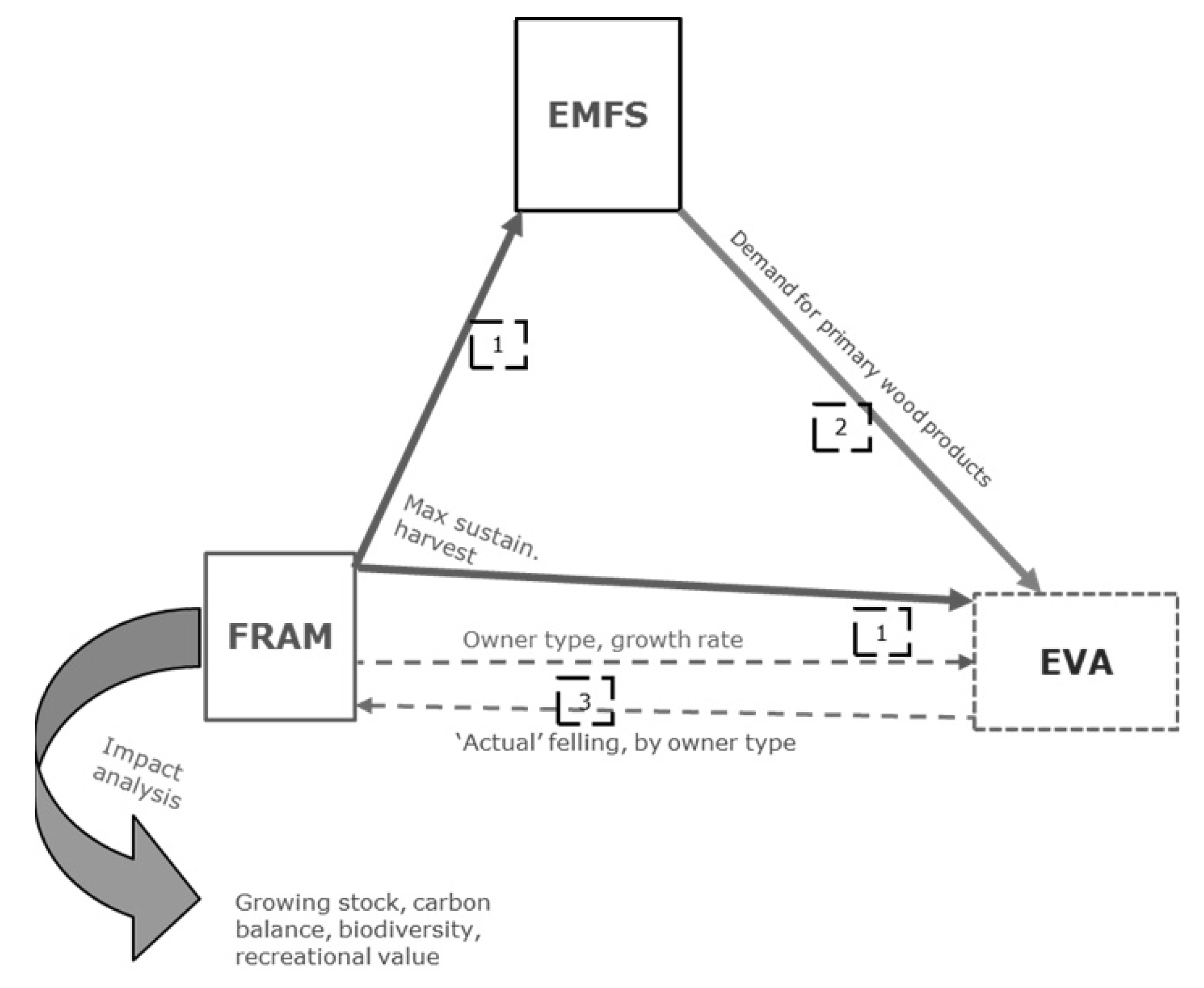
In this paper we consider a modeling framework, which departs from standard (European) ones, combining resources assessment and economic modeling. Indeed, the suggested approach applies, beside a forest resource assessment model (FRAM) and an economic model for the forest sector (EMFS), also a third model (EVA), which works as an intermediary between FRAM and EMFS, completing the integration between the two, and enriching the quality of the information transferred from one model to the other. Indeed, it is generally recognized that one of the drawbacks of the existing frameworks is that they are only partially integrated, since no feedback from the EMFS to the FRAM is foreseen.
This is obviously quite a relevant shortcoming, since even if the FRAM correctly provided as input to the EMFS the maximum amount that could potentially be harvested in a sustainable manner, multiple errors would propagate over time, if the actual quantity of harvested wood were arbitrarily set equal to this upper bound, without taking into account that the satisfaction of the demand might have required a lower harvesting level. Thus, EVA can complete the loop between the two models, using as inputs the maximum harvestable level from the FRAM, and the demand for wood primary products from the EMFS, and returning, as output, the amount effectively harvested to be ingested in the FRAM.
As will be further elaborated, EVA enriches the information returned to FRAM, since it also takes into account how forests are partitioned among forest owners differing as to a number of factors—psychological, social, cognitive, and emotional (henceforth “behavioral” factors)—that crucially influence individual harvesting decisions, and consequently total wood supply. These particular factors are modeled in a simple and intuitive way by means of preferences coefficients, such as the standard risk aversion coefficient, and the patience coefficient, that reflects the preference of the forest owner for preserving the forest for a longer time horizon versus (earlier harvesting and) earlier realization of the monetary revenues.
Obviously, the numerical assignments to the various parameters in EVA are to be regarded as informed estimates only. Another caveat is in order here: as knowledge concerning the distribution of forest land on different types of forest owners is generally quite scant, “expert judgment” is normally needed to allocate the forest resource on different owner types. These two, unrelated, sources of uncertainty makes frameworks as the one below most suited for policy scenario analysis, as scenario analysis is better equipped to deal with indeterminacies caused by ignorance than, e.g., extrapolating methods [10].
To explain the linkages between FRAM and EMFS more concretely, let us consider a FRAM that derives the total maximum harvestable level—given environmental and legal constraints—ingested by the EMFS as upper bound to the supply of primary products (Figure 1). Simultaneously, this information is also sent to EVA along with information regarding forest growth rate and owner type. EMFS derives the global forest sector equilibrium and sends the demand (at national or sub-regional level) for primary products to EVA. Given this information, EVA computes the amount to be harvested in order to maximize the utility from wealth of the respective forest owner, under the resource constraint provided by FRAM, and the requirement that the entire equilibrium demand derived in EMFS has to be satisfied. EVA’s results are then fed back into FRAM completing the loop from EMFS to FRAM (Figure 1).
Figure 1.
EVA as part of a DSS. Source: Rinaldi and Jonsson [9].
Figure 1.
EVA as part of a DSS. Source: Rinaldi and Jonsson [9].

3. Materials and Methods
Here follows a description of two of the three models belonging to the suggested (augmented) DSS. Indeed, in this paper, we elaborate only the linkage between FRAM, here EFDM, and EVA. This is just a technical simplification, which was voluntarily introduced in order to facilitate the interpretation of our results. Indeed in our framework, the role of the EMFS is to provide EVA with the demand for timber at any time step, however here we have rather preferred to consider a time-invariant demand, in order to better isolate the role played by the preference coefficients (and hence by forest owners’ heterogeneity) in shaping wood supply.
3.1. Expected Value Asymmetries: A Harvesting Behavior Model
Expected Value Asymmetries (EVA) is a multi-agent harvesting model for scenario analysis, which integrates forest resources assessment and economic equilibrium. The distinctive feature of EVA is that it allows considering alternative partitions of forest owners into (homogeneous) categories characterized by different behavioral factors, which might influence harvesting decisions, and henceforth total available timber supply. Such factors are modeled by means of two coefficients: the standard risk aversion coefficient, and the patience coefficient, already introduced in [9], which reflects the preference of the forest owner for preserving the forest for a longer time horizon versus earlier harvesting and earlier realization of the monetary revenues.
These parameters shape forest owners’ preferences and subsequently influence their harvesting behavior. In particular, for any given partition, EVA uses as input the total maximum harvestable level and the equilibrium total demand for wood to derive the optimal amount that needs to be harvested by each (forest owner) category in order to satisfy the entire equilibrium demand. By “optimal” we mean that forest owners are maximizing their individual utility, or, equivalently, that they are satisfying their preferences as best as they can, and, therefore, they are taking into account their own particular behavioral factors.
Another distinctive element is the availability of information. More precisely, EVA assumes that forest owners have some information concerning the riskiness of the economic environment (or at least a perception of it) and that they formulate personal conjectures concerning the dynamics of timber prices and of the demand. Obviously, different categories might have different information, which again affects harvesting decisions and total supply.
Theoretical Foundation
We start by defining N possible preferences-based types of forest owners, and we assume that for each preference type n, there are 3 representative forest owners, y, i and o, whose forest stock is “young”, “intermediate age”, and “old”, respectively. Trees owned by forest owners of type n belong to one of the tree forest stocks, and hence to forest owner y, i, or o, depending on their age class. Each preference-type n is characterized by two (preference) parameters: the customary coefficient of risk aversion ρn, and the degree of patience with respect to postponing the income deriving from harvesting, θn.
In particular, we assign weights 1 − θn and θn to earlier and later monetary wealth from timber sale, respectively. The use of the pair (1 − θn, θn) allows us to express the degree of patience with respect to monetary outcomes realized in the future (as opposed to earlier ones), in particular, if θn = 0, the landowner only values monetary outcomes realized from earlier timber sales, whereas, when θn = 0.5, monetary outcomes from current and future sales are equally valued. A higher degree of patience (0.5 ≤ θn < 1) signalizes that the forest owner assigns the forest additional value beside the one provided by timber sales, and therefore is keen on carrying a larger forest stock to the future, even if this might not be optimal from a pure monetary perspective. This might, for example, be the case if the forest is part of an inheritance, if it has high ecological value, or if it provides non-monetary amenity services.
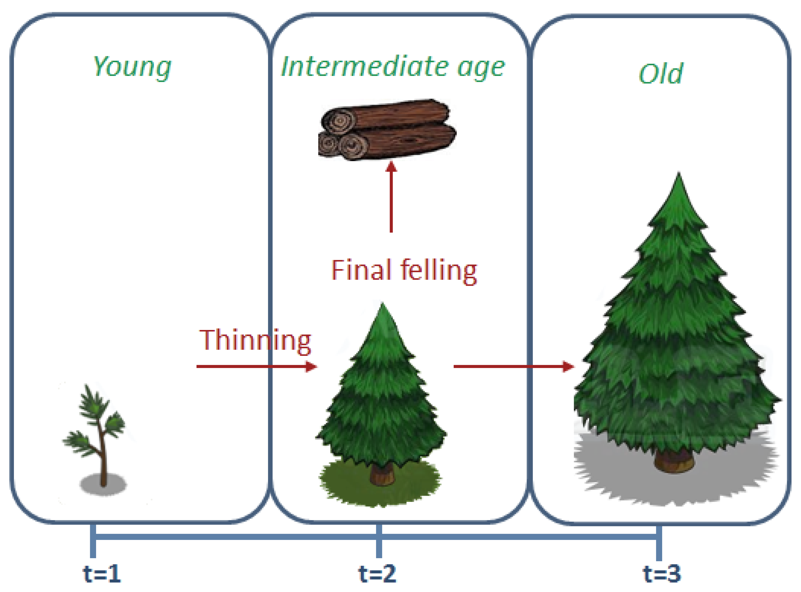
Time is discrete and, for simplicity, we assume that the interval between each time step coincides with the time necessary for a tree to move from one category to the following, namely for “young” trees to become of “intermediate age”, and for trees of “intermediate age” to become “old”. Trees belonging to the “young forest”, y, can only be thinned up to a certain percentage of the initial growing stock, while no constraint is set for trees belonging to categories i and o. Specifically, forests in the o category at time t can be partially clear-cut, and trees that are not harvested will increase the growing stock in category o available in the next period t + 1. The remaining part of the growing stock in category o available in the next period t + 1 originates from the trees available in category i in the current period t, which have not been harvested. Finally, forests of category y in the current period t are thinned at time t and they will constitute category i in the next period t + 1 (Figure 2).
Figure 2.
State transitions in the modeling.

In the following we assume that only categories y and i actively decide how much to harvest from their forests, while the third category o harvests only if the demand is still unsatisfied given the optimal choices of categories y and i. Specifically, we assume that each of the 2N decision-making forest owners from categories y and i wants to maximize the utility derived from individual final wealth, by choosing how much to harvest from the owned forest stocks.
Forest owners in category i will choose the optimal percentage of their forest to be clearcut, while forest owners in category y will choose the thinning level in the current period t, and also the percentage of the forest they plan to clearcut in the following period t + 1. However, the latter could be possibly revised in light of the equilibrium price realized at time t and the new demand at time t + 1. We also assume that forest owners in categories y and i all have the same utility index U, with exponential form and constant risk-aversion ρn, that is, U = −exp(−ρnwnoa), where wnoa represents final wealth for an individual belonging to forest owners’ type n, whose initial forest stock belongs to category a = y, i. We denote the individual forest stock of a generic forest owner of type n and category a (a = y, i, o) and the corresponding amount to be harvested at time t, by Qna and xna,t, respectively.
Given the (inelastic) demand for wood Dt, the harvested quantities xna,t (a = y, i, o, n = 1,2,… N) are sold on the timber market at price pt, and the proceeds from timber sales are invested in a risk free bond with periodical gross return 1 + r. Finally, in order to assign a potential monetary value also to trees that are not harvested, we set to pt the unitary value of the entire growing stock of old forests.
Without loss of generality, in order to simplify notation, let us fix t = 1, so that forest owners from category y want to maximize the utility derived from wealth available at time t = 3, and those from category i the one available at time t = 2. More precisely, in order to take into account the fact that forest owners might have different degrees of patience with respect to the timing at which monetary incomes realize (as also reflected in the patience coefficient θn), we will consider instead the utility of final weighted wealth wnoy = θnp3xno3 + (1 − θn)[p1xny1(1 + r)2 + p2xni2(1 + r)] for category y, and wnoi = θnp2xno2 + (1 − θn)[p1xni1(1 + r)] for category i. Thus, the largest time horizon considered in the decision problem is of three periods, as it is for the y category of forest owners.
When the landowner makes his/her harvesting decision, the demand-level, Dt, and the timber prices are not known. However, all landowners know that prices pt are derived as equilibrium, while they hold beliefs concerning the distributions of Dt and the dynamic of prices. In particular, both Dt and pt are driven by a stochastic common component εg, which can be thought of as a long-run economic shock affecting all periods (an example could, e.g., be a realization of the bioeconomy, creating a long-term increase in the demand for wood), and a time contingent shocks, εt.
We denote by ε1, ε2, and ε3, contingent shocks at time 1, time 2, and time 3, respectively. The variance of εg, σg2, can be thought of as a measure of economic risk. The three shocks ε1, ε2, and ε3 are mutually independent, and, in addition, they are also independent from εg. Therefore, they represent specific time contingent shocks exclusively affecting time 1 (ε1), time 2 (ε2), and time 3 (ε3), respectively. Hence, σ12, σ22 and σ32 can be thought of as measures of time specific risk. To make examples, one can imagine a temporary variation in exchanges rates affecting timber demand, or a provisional reduction in the activity of a major sawmill in the area in question.
More specifically, we assume D1 = D(1 + εg) + ε1, D2 = D(1 + εg) + ε2, and ptp - 1(1 + m) + εg + εt, where m, D∈ℜ++, t = 2,3, εg ~N(0, σg2), ε1 ~N(0, σ12), ε2 ~N(0, σ22), ε3 ~N(0, σ32). The constant D can be thought of as base demand level, and the percentage variation from it (εg) depends on the overall long-run economic development. In addition, the forest sector (and henceforth the demand) can also be hit by a time-contingent shock εt, which will have no residual effect on the following period, time t + 1. The price at time t depends on the equilibrium price at time t − 1, the long-run economic shock, εg, and the time specific shock at time t, εt. For concreteness, we assume that m > r, for example one can imagine that m is a fixed inflation rate and, in absence of any additional information, forest owners/managers might assume that future timber prices will adjust for inflation.
Given the amount harvested at time 1, xna1, the stock available at time 2, Gna2, is uniquely defined by the growth function and the initial forest endowment Qna. For simplicity we will consider a linear growth function. Obviously such an assumption violates the concavity requirement, however, our analysis does not crucially rely on this specification, which instead allows for a reduction in the notational and computational complexity of the model. Therefore, we assume:
where kna is a positive constant.
Finally, we assume that all forest owners have a preference for sustainable forms of management, and/or that there are legal instruments to enforce it. In order to accommodate for this, we assume that, when deciding upon optimal harvesting levels, i forest owners take into account also an inter-temporal sustainability condition aimed at guaranteeing that the stock of old forests is not completely depleted over time. Specifically, for each category a, we introduce the additional constraint:
where c is a positive constant.
For y forest owners, the initial maximization problem consists in choosing optimal current timber supply xny1, and, provisionally, future timber supply xni2, in order to maximize the utility from final weighted wealth wnoy under the growth constraint Equation (1), given the available initial information Ω, represented by the beliefs concerning the demands’ distribution and the prices’ dynamics. Hence, the maximization problem is:
under the constraint:
where E[·] denotes the expectation operator and β is an upper bound to the percentage of the growing stock that can be initially thinned.
Given the actual realizations of the equilibrium price p*1 and of the demand D1, forest owners y update their beliefs concerning the price dynamics and the future expected demand, and choose the optimal actual harvesting level for the next period. In particular, if the forest owners still believes into the conjectures D2 = D(1 + εg) + ε2, and pt = pt - 1(1 + m) + εg + εt, then both p*1 and D1 work as disturbed signals of the aggregate shock εg, so that beliefs can be updated in a standard Bayesian fashion (we refer the interested Reader to [9] for additional insights on signals and updated priors in a simpler setting). Otherwise, the forest owners might simply reconsider the values assigned to the parameters m, D, σg2 and σt2, t = 2,3.
In a similar fashion, i forest owners choose optimal current timber supply xni1 to maximize the utility from final weighted wealth wnoi under the growth constraint Equation (1), given the initial information Ω, that is:
under the constraint Equation (2) and
In period 2, the previously young forests becomes of intermediate age, and, given the new information Ω1 provided by the equilibrium (p*1, D1), the optimal harvesting level xni2, is chosen solving the optimization problem Equations (5) and (6).
Given the normality and the independence assumptions concerning the shocks, wnoa| Ω is also normally distributed. Further, the utility index is a standard constant risk aversion exponential utility, so that the expected utility of wnoa given information Ω is a strictly increasing transformation of the kernel E[wnoa| Ω] – 0.5ρnVar[wnoa| Ω].
The first order conditions associated to the maximization problems above express the optimal harvesting schedules xn*y1 and xn*i1 as functions of the time 1 price p1 and under the assumption that the price dynamics is described by pt = pt - 1(1 + m) + εg + εt, thus xn*y1 (p1) and xn*i1 (p1). That is, for any possible realized equilibrium price p*1, xn*y1 (p*1) and xn*i1 (p*1) return the optimal harvesting levels for categories y and i. The equilibrium price p*1 and the corresponding equilibrium supply levels xn*y1 (p*1) and xn*i1 (p*1) are then computed by equating the sum over the groups of the supply functions xn*y1 (p1) and xn*i1 (p1) to the realized demand D1, and satisfying the possible excess demand through harvesting from old forests xn*o1 (We refer the reader to Rinaldi and Jonsson [9] for a complete derivation of all these results).
In the following period young forests becomes of intermediate age, and unharvested forests of intermediate age join the set of old unharvested trees to form the time t + 1 growing stock of old forests and the optimization problem just repeats.
3.2. European Forestry Dynamics Model (EFDM)
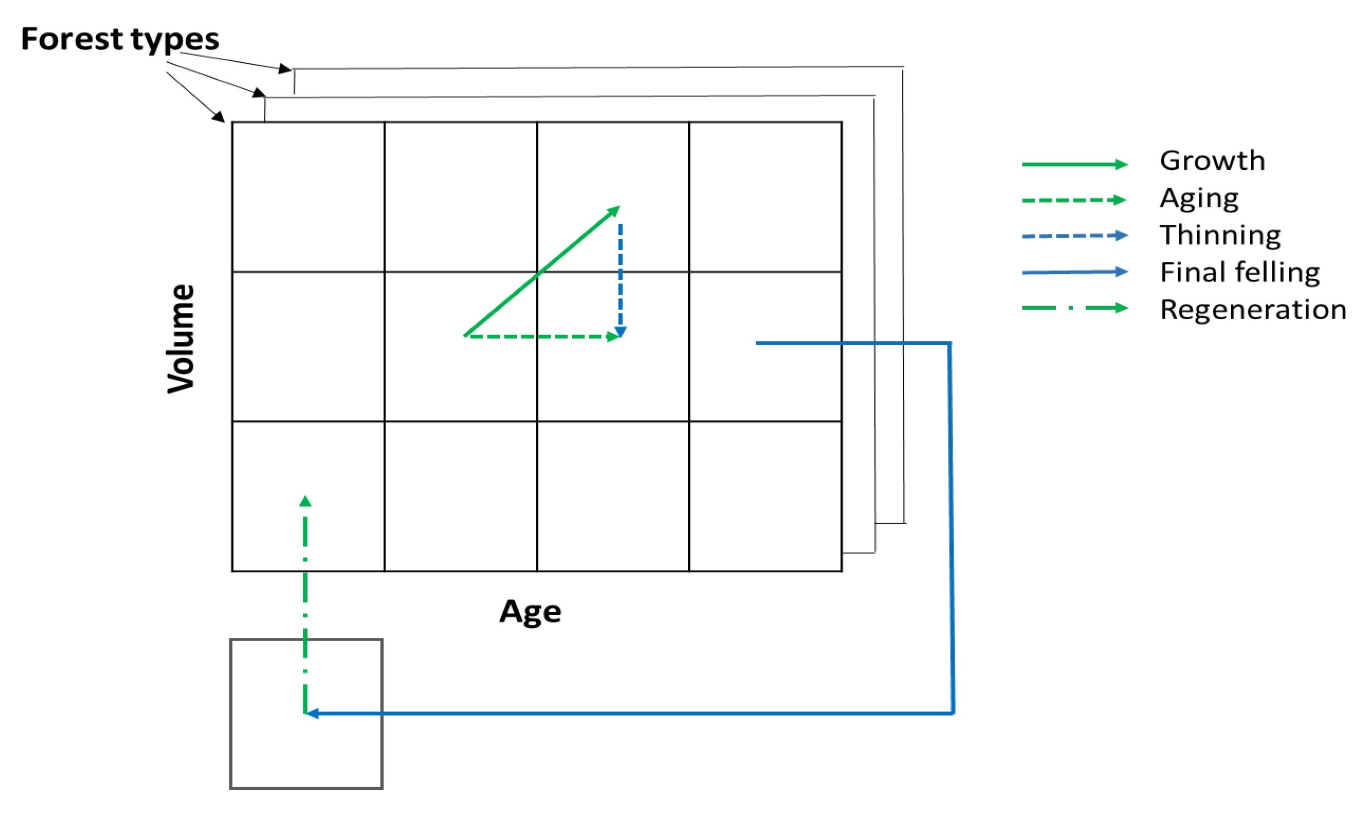
EFDM [11] is an area-based matrix model, meaning that forest areas are transiting between elements of a set of fixed states (Figure 3). The transitions are controlled by the initial state and the activities given for each state. The concept is based on the ideas presented by Sallnäs [12].
Figure 3.
An area matrix state transition model. Adapted from: Schelhaas et al. [13].
Figure 3.
An area matrix state transition model. Adapted from: Schelhaas et al. [13].

Given a set of fixed states S, let’s denote by X0 the initial area distribution over the states, and by P the transitions between different states (S) guided by the activities A (defined over S).
When applied to even-aged forests, the set S is usually defined by classes for age and standing volume. A common S is associated with all the different “forest types” which in turn are defined by for example region, species, site quality and/or owner. In the first phase of model development, the concept has been tested in five countries. In all cases, the national forest inventory (NFI) knowledge about forest states, management and their interrelations was utilized in the model definition and estimation.
The initial state matrix X0 was estimated using NFI plot data, while the transition matrix P was estimated using two consecutive measurements of NFI plots, increment measurement of NFI plots, or growth information from pre-existing functions. Estimation of the X matrix is a simple classification, while the P matrix is estimated using a Bayesian procedure. The activity matrix A is given, in one form or the other, by relying on national expertise. In the Swedish test case used in this paper, the set S was defined by 10 (11) volume-classes and 33 (34) age-classes for 60 different “forest types” (five regions, four site classes and three species). The extra classes inside parenthesis are used to handle bare land.
3.3. Data and Simulation Assumptions
3.3.1. Forest Data: Distribution of Forest Area on Owner Types, Assignment of Cohorts Available for Harvesting, Harvesting probabilities
The forest data concerns the region of southern Sweden, Götaland. On average, this region accounts for slightly more than one third of the annual harvest volume of Sweden [14]. The dominant ownership class is non-industrial private forest owners (NIPF), accounting for about 78% of the forest area [15] and over 80% of the annual harvested volume in the region [14]. Private sector companies account for slightly less than seven percent of the forest area [15], but almost eleven percent of the annual harvested volume [14]. Public and other type of ownerships make up the remaining share of forest area and annual harvest (ibid.).
To meet the specific objective of capturing the importance of forest owner heterogeneity on the development of forest resources and timber market, we created a special data set. Using the three owner types present in the NFI-data: public, company, and private, we allocated the factual forest of Götaland, as depicted by the NFI-data, evenly to the three owner types. This means that initially the owner types have identical forest holdings. In order to set up the model framework we also defined 4 cohorts of forest, of which 3 served as information carriers between the different models.
- 1
- Forest too young to be harvested (0–50 years);
- 2
- Medium-aged forests that can be thinned (51–60 years), corresponding to y in EVA;
- 3
- Older forests that can be final felled (61–70 years), corresponding to i in EVA;
- 4
- Old forest that can be final felled (71-years), corresponding to o in EVA.
The total volume in each of cohorts 2–4 for the different owner types was transferred from EFDM to EVA at each iteration, and information about volume harvested in the cohorts/owner types was sent back. For the sake of simplicity, cohorts 2 and 3 were assumed to have a width of 10 years, coinciding with the time step used in the model runs. The increment rates for the cohorts were deduced directly from the EFDM model. For all owner types a common activity pattern were defined based on the Swedish forest management “school-book”, in which legal restrictions are included. This pattern could then be shifted upwards or downwards separately for each cohort and owner type to meet a specified harvest level.
As already mentioned, we considered a time-invariant timber demand, which was set to 280 million m3, based on historic harvest levels in Götaland, see [14]. Here we do not consider the allocation of growing stocks on different tree species. Provided that the harvesting demand can be given as species specific, there is no principal problem in accounting for this, given the set of S, as described in the previous section.
3.3.2. EVA: Forest Owner Typologies used and Numerical Assignment of Owner-Type Parameters
In creating forest owner typologies, we draw on previous research on the topic [4,5,6,7,8]. Given that the forestland in Götaland has three main owner categories, and building in particular on the typology developed in [5], we consider the following owner types: Economic Man (EM), Elderly Couple (EC), and Multi-objective (MO). In choosing the characteristics of each category, we aimed at achieving sufficient variation as well as a continuum regarding objectives, and associated risk aversion and patience with respect to monetary outcomes, specifically:
- Economic Man (EM), which here corresponds to private sector companies, has as overriding objective of the maximization of the monetary value of the forest, no matter if it comes from present or future timber sale, equivalently, the patience coefficient θEM is at intermediate level. Risk aversion (ρEM) is also at intermediate level.
- Elderly Couple (EC), which here corresponds to NIPF, has as a main purpose to leave a forest holding in as favorable (economic) condition as possible for their children. Consequently, the value of wealth from current timber sale is low (equivalently, patience (θEC) is high) and risk aversion (ρEC) concerning future timber market conditions is high.
- Multi-objective (MO), here representing public ownerships, values both monetary and amenity (non-timber) benefits of forest holdings. Risk aversion (ρMo) is at intermediate/high levels and, due to amenity valuation, patience θMo with respect to future timber sales is fairly high.
Next, we rank the three owner types according to risk aversion (ρ) and the degree of patience with respect the future (θ). From the lowest to the highest risk aversion (ρ) we have: Economic Man, Multi-objective, and Elderly Couple (ρEM ˂ ρMo ˂ ρEC). Similarly, from the highest coefficient θ to the lowest: Elderly Couple, Multi-objective, and Economic Man (θEC > θMo > θEM).
It should be noted that the ranking and the numerical assignment to the various parameters are informed estimates only, based on a number of studies of forest owner attitudes [2,3,4,5,6]. For example, the high degree of the patience of the Elderly Couple is derived from Ingemarson et al. [5], where the category, or objectives cluster, “traditionalists”, which inspired our Elderly Couple, is the one that to the largest extent expects children or other relatives to take over the forest estate. Accordingly, we assume that Elderly Couple, wishing to hand over a well-stocked forest holding, are less concerned with wealth from current timber sales.
In addition, a number of simplifications are implicitly assumed, such as inelastic demand and the absence of any budget or consumption requirements for the forest owners. Further, the circumstance that timber from older forests is, on average, higher valued is not directly accounted for. We acknowledge the importance of these simplifications; however, their purpose is to render the problem more tractable both at theoretical and at numerical level. Relaxing some, or all, of these assumptions would in principle be possible, but it would come at the cost of greater complexity, especially in the evaluation of the cause and effects relationship when interpreting the results. In future research, we will expand the current framework (and henceforth we will relax some of the above assumptions) to focus on some interesting issues temporarily disregarded by the current analysis, such as the price formation mechanism, which, for example, would require us to relax the assumption of inelasticity of the demand for wood.
The specific numeric assignment of the various parameters is not important compared to their relative ordinal ranking. However, since all groups maximize the utility from economic wealth only, and since they only care about economic risk, we have assigned the type-specific values of the risk aversion coefficient (ρ) drawing on standard economic literature. In particular, the coefficient ranges from 3 to 11 (ρEM = 3, ρMo = 7, ρEC = 11). Indeed, as discussed in [16], most individuals have risk aversions between one and ten, as it is for EM and EC, while a minority display higher values, as for EC to whom we wanted to assign an unusually high degree of risk aversion.
Since weighted wealth wnoa is defined as a linear combination between earlier and later monetary outcomes using (1 − θn) and θn as weights, θn necessarily lies between 0 and 1, and equal weighting implies θn = 0.5, which in our example corresponds to EM. The other values have been assigned to reflect higher, but not extreme (i.e., θn < 1), patience, in particular θEM = 0.5 ˂ θMo = 0.6 ˂ θEC = 0.75.
4. Results and Discussion
Table 1, Table 2 and Table 3 depict the growing stocks before harvest and harvest levels in the three cohorts that can be thinned (y, medium-aged forest) and final felled (i: older forest, and o: old forest), respectively, for the three different owner types (for typographic reasons the category “Multi-objective” is labelled as “Multi-Obj.”). It is interesting to notice that the harvesting behavior of the three forest owner types differ consistently for what concerns the optimal harvesting of the i cohort, while only minimal differences are noticeable for harvesting levels of y forests. The reasons beyond this particular pattern are mainly two: first of all, all types in cohort y are constrained by the same upper bound and the constraint is indeed binding for all three typologies. Secondly, risk aversion and patience degree have the opposite effect on forest owners’ decisions. Specifically, a higher coefficient of risk aversion determines a strong tendency to harvest in earlier periods for protective purposes, while a higher degree of patience implies a strong tendency to postpone harvesting later in time.
Comparing the three typologies of the paper, it is easy to notice that ρEM ˂ ρMo ˂ ρEC, which, ceteris paribus, would imply that the maximum (minimum) supplied quantity would be harvested by the EC (EM), but also θEC > θMo > θEM, which would imply exactly the opposite ranking. Hence, at least in principle, the overall effect on harvesting level is unpredictable (as it is for y forests). However, as the forest gets older, that is, as it moves from cohort y to cohort i, the tradeoff between earlier and later harvesting reduces. This can easily be seen by comparing the expression for wnoy, wherein two cash flows are weighted by the coefficient (1 − θn), or, equivalently, considered earlier realizations of the monetary revenues, with the one for wnoi, wherein only one cash flow is so. If such tradeoff is reduced, then the prevailing effect is the one generated by risk aversion, which determines the ranking xECi2 > xMoi2> xEMi2.

| Growing Stock before Harvesting (million m3), Time 1 | Equilibrium Harvest Levels (million m3), Time 1 | ||||||||
|---|---|---|---|---|---|---|---|---|---|
| Types | Multi-Obj. | Economic Man | Elderly Couple | SUM | Types | Multi-Obj. | Economic Man | Elderly Couple | SUM |
| Cohort y | 29.01 | 29.01 | 29.01 | 87.03 | Cohort y | 8.7 | 8.7 | 8.7 | 26.1 |
| Cohort i | 31.21 | 31.21 | 31.21 | 93.63 | Cohort i | 17.09 | 0.01 | 27.01 | 44.11 |
| Cohort o | 129.06 | 129.06 | 129.06 | 387.18 | Cohort o | 72.97 | 91.22 | 45.61 | 209.80 |
| TOTAL | 189.28 | 189.28 | 189.28 | 567.84 | TOTAL | 98.76 | 99.92 | 81.32 | 280.00 |
| Growing Stock before Harvesting (million m3), Time 2 | Equilibrium Harvest Levels (million m3), Time 2 | ||||||||
|---|---|---|---|---|---|---|---|---|---|
| Types | Multi-Obj. | Economic Man | Elderly Couple | SUM | Types | Multi-Obj. | Economic Man | Elderly Couple | SUM |
| Cohort y | 50.68 | 50.68 | 50.69 | 152.05 | Cohort y | 15.20 | 15.20 | 15.21 | 45.61 |
| Cohort i | 30.35 | 30.35 | 30.34 | 91.04 | Cohort i | 14.93 | 0.00 | 30.34 | 45.27 |
| Cohort o | 86.51 | 86.87 | 106.64 | 280.02 | Cohort o | 65.78 | 82.22 | 41.11 | 189.11 |
| TOTAL | 167.54 | 167.90 | 187.67 | 523.11 | TOTAL | 95.91 | 97.42 | 86.66 | 279.99 |
| Growing Stock before Harvesting (million m3), Time 3 | Equilibrium Harvest Levels (million m3), Time 3 | ||||||||
|---|---|---|---|---|---|---|---|---|---|
| Types | Multi-Obj. | Economic Man | Elderly Couple | SUM | Types | Multi-Obj. | Economic Man | Elderly Couple | SUM |
| Cohort y | 72.97 | 72.98 | 73.00 | 218.95 | Cohort y | 21.89 | 21.89 | 21.90 | 65.68 |
| Cohort i | 49.61 | 49.61 | 49.61 | 148.83 | Cohort i | 18.90 | 6.91 | 36.21 | 62.02 |
| Cohort o | 44.98 | 45.94 | 76.71 | 167.63 | Cohort o | 52.97 | 66.21 | 33.11 | 152.29 |
| TOTAL | 167.56 | 168.53 | 199.32 | 535.41 | TOTAL | 93.76 | 95.01 | 91.22 | 279.99 |
Table 4 presents total harvest levels over all three periods. As already pointed out, the differences in harvest (thinning) volume between the three owner types in cohort y are barely noticeable, whereas instead differences are pronounced in cohorts i and o. EM, harvesting much less than the other two owner types in i, instead harvests considerably more in the oldest cohort. These results as to harvest levels are well in line with what could be expected, given the characteristics of the owner types. Thus, EM, having the highest total harvest level, concentrates harvesting to the cohort with the lowest growth rate and corresponding lowest economic return. Conversely, EC has the lowest total harvest level and also the lowest harvest volume in the oldest cohort, while MO is in between both these extremes (though considerably closer to EM).
| Types | Multi-Obj. | Economic Man | Elderly Couple | Sum |
|---|---|---|---|---|
| Cohort y | 45.79 | 45.79 | 45.80 | 137.38 |
| Cohort i | 50.93 | 6.92 | 93.562 | 151.41 |
| Cohort o | 191.74 | 239.66 | 119.83 | 551.21 |
| TOTAL | 288.44 | 292.36 | 259.19 | 840.00 |
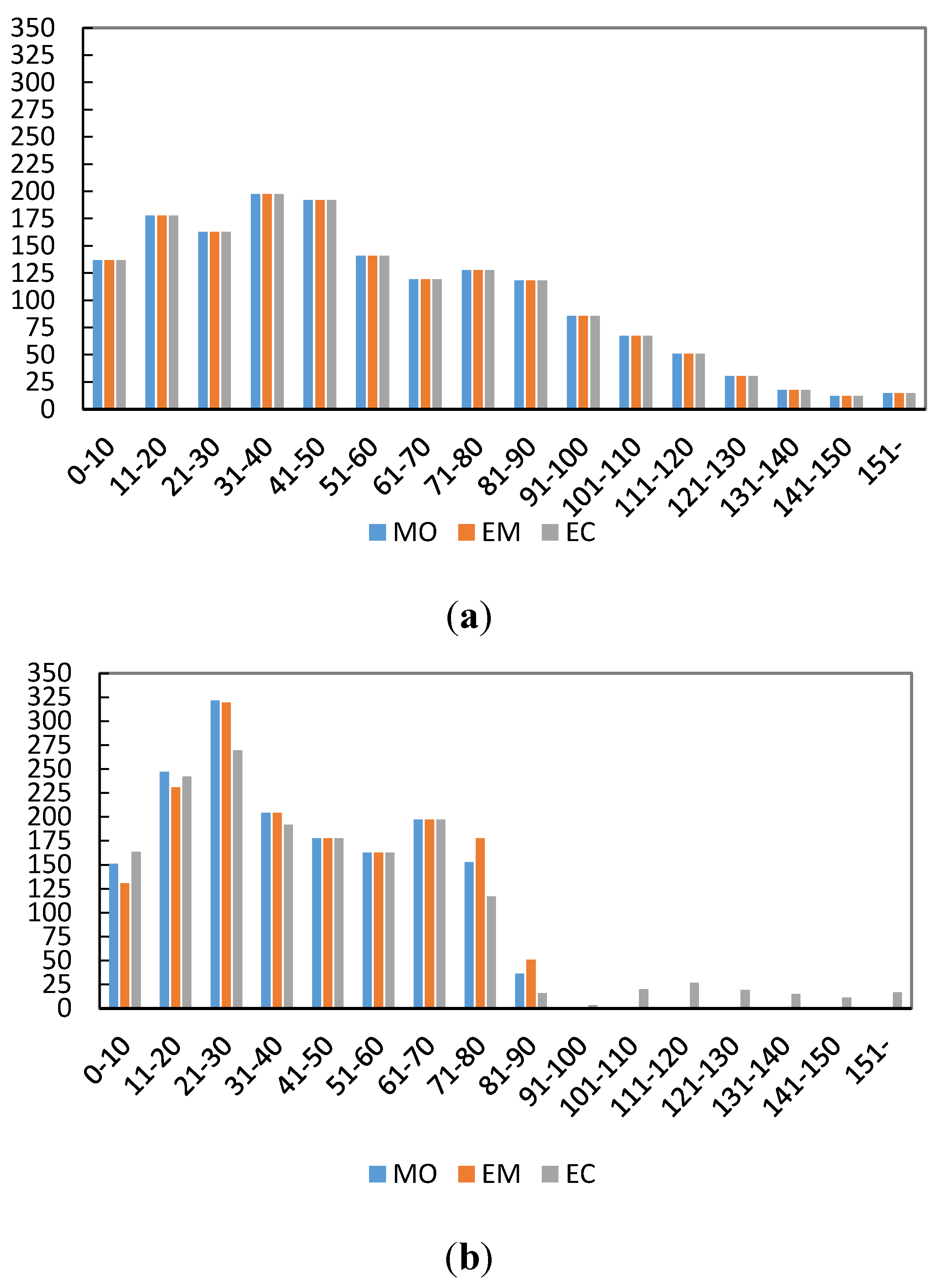
It is of interest to assess what forest owner heterogeneity means in terms of development of the forest state over time. Figure 4 illustrates the distribution of the forest area on age classes, initially and after thirty years, for the three owner types. The age class distribution is quite similar for MO and EM. Though harvesting less than EM in the oldest cohort, MO still has a slightly smaller area of old forest, as the “in-growth” from the intermediate cohort is small enough to cancel out the effect of a lower harvesting level in the oldest cohort. For both owner types there is a considerable “rejuvenation” of the forest resource.
Figure 4.
Forest state: age-class distribution of the forest area (thousands of hectares). (a) Initial forest state; (b) Forest state after 30 years.
Figure 4.
Forest state: age-class distribution of the forest area (thousands of hectares). (a) Initial forest state; (b) Forest state after 30 years.

Compared with the former two, EC stands out as being the only owner type still having some forest area in the highest age classes. Even so, after thirty years EC also has a larger area of young forest than the initial one. EC has the largest area in the age classes where final felling is possible of all three owner types after thirty years. However, this area is still 200 thousand hectares lower than the initial one. This is due to a considerable reduction of forest area in the age classes above 80 years of age. However, more importantly, unlike MO and EM, for EC the total growing stock in the three “harvestable cohorts”—i, y, and o—is higher already before the third harvest than the initial one, as can be seen in Table 3. This can be seen as EC realizing the objective of leaving the forest holding in as favorable condition, in an economic sense, as possible.
Comparing Figure 4a,b, it is evident that the age-class distributions after thirty years of simulation do not coincide with the one describing the initial state. Since an age-class distribution can be regarded as reflecting historical management (including the absence of activity), it could be concluded that the management prescribed by EVA is not identical to historical management leading up to this initial state. The most apparent difference is that EVA prescribes harvest in the old forest to a higher degree than what has been applied historically, still within the limits of what can be sustained without diminishing total growing stock, though. This could be due to the circumstance that a considerable percentage of forest owners are quite passive in their management, something that is not considered in the current study.
5. Conclusions
The current study suggests a framework to overcome the shortcoming of current forestry decision support systems (DSS) of not fully accounting for forest owner heterogeneity. Specifically, we propose an approach for integrating forest resources assessment and economic modeling of harvesting behavior. The suggested framework takes into account forest owners’ heterogeneity as regards objective, risk attitude, and patience relative to the timing of harvesting (and, consequently, also of the realization of monetary revenues).
The modeling results presented suggest that the approach put forward, though stylized, holds promise as regards accounting for forest owner behavior in simulations of forest resources development. Hence, forest owner heterogeneity makes the distribution of forestland on owner types non-trivial, affecting harvesting intensity and, subsequently, inter-temporal forest development.
The presented framework could be further elaborated in several ways: for example it would be interesting to work with a higher number of owner types, especially to split the EC group into different types reflecting the intragroup variation inside NIPF. Furthermore, the allocation of forest areas, and consequently forest state, should, if possible, be based on data rather than assumptions. Also the limitation to consider only three cohorts, each with redefined management options, could be relaxed.
Another interesting expansion is the introduction into the framework of policy, and the analysis of the effects of forest owner heterogeneity on policy impact. The present framework is particularly suitable for this scope, since it allows policy to be represented through signals, as also anticipated in [9]. This type of representation is interesting, since it allows the policy to be perceived as “good (news)” or “bad (news)” from the forest owner perspective. It also accounts for the circumstance that policy-effects might be perceived as long lasting and/or time contingent, and also for the specific degree of confidence of individual forest owners/managers (in the policy maker).
As it already appears here, the modeling approach could also alternatively be used to design an optimal forest management scheme from an owner perspective, taking into accounts his/her specific characteristics, given ecological/sustainability requirements.
The present study includes several simplifications, already detailed, in order to focus on the basic issue: how to capture the impact of forest owner heterogeneity on forest development. However, the purpose here is not to launch a fully operative tool for policy-analysis, but rather to propose and demonstrate a concept for how forest owner specific harvesting behavior can be accounted for when modeling forest resource dynamics, thus providing an augmented DSS.
On a general note, decreasing the degree of uncertainty related to lacking information—as to (i) attitudes and objectives of forest owners, and how they are manifested in harvesting behavior; and (ii) the distribution of forest land on different types of forest owners—would enhance DSSs as the one outlined here and thus contribute to informed policy making. The approach taken in the EFDM, i.e., consulting national expertise, is therefore a most fruitful way of increasing the knowledgebase when constructing pan-European DSSs.
List of Symbols
| N | total number of preferences-based types of forest owners (in the paper N = 3: Economic Man (EM), Elderly Couple (EC), and Multi-objective (MO)) |
| n | index generically identifying a specific type of forest owner (in the paper n = EM, EC, MO) |
| y | index for “young” forest stocks |
| i | index for “intermediate age” forest stocks |
| o | index for “old” forest stocks |
| ρn | coefficient of risk aversion for a forest owner of type n (n = EM, EC, MO) |
| θn | degree of patience with respect to postponing the income deriving from harvesting for a forest owner of type n (n = EM, EC, MO) |
| t | time index |
| U | utility index (in the paper exponential utility) |
| wnoa | weighted final wealth for an individual belonging to forest owners’ type n, whose initial forest stock belongs to category a (a = y, i). In particular, wnoy is weighted final wealth for an individual belonging to forest owners’ type n, whose initial forest stock is “young” and wnoi is weighted final wealth for an individual belonging to forest owners’ type n, whose initial forest stock is “intermediate age” |
| Qna | forest stock of a generic forest owner of type n and category a (n = EM, EC, MO and a = y, i, o) |
| xna,t | harvested quantities at time t by a generic forest owner of type n and category a at time t (n = EM, EC, MO and a = y, i, o). Specifically, for a y forest owner at time 1, current harvest is xny1, while future timber supply is xni2. For a i forest owner at time 1, current harvest is xni1 |
| Dt | demand at time t |
| D | base demand level |
| pt | timber price at time t |
| m | expected growth rate of timber prices |
| r | rate of return of the risk free bond |
| εg | long-run economic shock affecting all periods |
| σg | variance of εg |
| εt | time t contingent shocks, specifically ε1, ε2, and ε3 are the time contingent shocks at time 1, time 2, and time 3, respectively |
| σt2 | variance of the time t contingent shocks εt, specifically σ12, σ22 and σ32 are the variances of ε1, ε2, and ε3, respectively |
| Gna2 | Forest growing stock available at time t = 2 for a forest owner of type n and category a at time t (n = EM, EC, MO and a = y, i, o) |
| kna | growth rate of a forest of category a belonging to a forest owner of type n (n = EM, EC, MO and a = y, i, o) |
| c | positive constant. 0 < c ≤ 1 |
| Ω | initial information |
| E[·] | expectation operator |
| β | upper bound to the percentage of the growing stock that can be initially thinned |
| p*1 | equilibrium price at time t = 1 |
| Ω1 | information available after the first period, provided by the equilibrium (p*1, D1) |
| xn*y1 | optimal harvest level at time t = 1 for the owner of type n of a young forest stock, given the realized equilibrium price p*1 |
| xn*i1 | optimal harvest level at time t = 1 for the owner of type n of an intermediate age forest stock, given the realized equilibrium price p*1 |
| xn*o1 | optimal harvest level at time t = 1 for the owner of type n of an old forest stock, given the realized equilibrium price p*1 |
Conflicts of Interest
The authors declare no conflict of interest. The opinions expressed herein are those of the authors and do not necessarily reflect the views of the European Commission.
References
- Bliss, J.C.; Martin, A.J. How tree farmers view management incentives. J. For. 1990, 88, 23–29, 42. [Google Scholar]
- Karppinen, H. Values and objectives of non-industrial private forest owners in Finland. Silva Fenn. 1998, 32, 43–59. [Google Scholar] [CrossRef]
- Kline, J.D.; Alig, R.J.; Johnson, R.L. Fostering the production of nontimber services among forest owners with heterogeneous objectives. For. Sci. 2000, 46, 302–311. [Google Scholar]
- Boon, T.E.; Meilby, H.; Thorsen, B.J. An empirically based typology of private forest owners in Denmark—Improving the communication between authorities and owners. Scand. J. For. Res. 2004, 19, 45–55. [Google Scholar] [CrossRef]
- Ingemarson, F.; Lindhagen, A.; Eriksson, L. A typology of small-scale private forest owners in Sweden. Scand. J. For. Res. 2006, 21, 249–259. [Google Scholar] [CrossRef]
- Favada, I.M.; Karppinen, H.; Kuuluvainen, J.; Mikkola, J.; Stavness, C. Effects of timber prices, ownership objectives, and owner characteristics on timber supply. For. Sci. 2009, 55, 512–523. [Google Scholar]
- EUwood—Real Potential for Changes in Growth and Use of EU Forests. Methodology Report; Hamburg University: Hamburg, Germany, 2010. Available online: http://ec.europa.eu/energy/renewables/studies/doc/bioenergy/euwood_methodology_report.pdf (accessed on 15 September 2013).
- Rinaldi, F.; Jonsson, R. Risks, Information and Short-Run Timber Supply. Forests 2013, 4, 1158–1170. [Google Scholar] [CrossRef] [Green Version]
- Rinaldi, F.; Jonsson, R. Information, multi-faceted forest ownership and timber supply. For. Res. 2014, 3, 1–9. [Google Scholar]
- Raskin, P.D. Bending the curve: Toward global sustainability. Development 2000, 43, 67–74. [Google Scholar] [CrossRef]
- Packalen, T.; Sallnäs, O.; Sirkiä, S.; Korhonen, K.T.; Salminen, O.; Vidal, C.; Robert, N.; Colin, A.; Belouard, T.; Schadauer, K.; et al. The European Forestry Dynamics Model (EFDM); JRC Scientific and Policy Reports; European Commission Joint Research Centre: Ispra (VA), Italy, 2013; p. 16. [Google Scholar]
- Sallnäs, O. A Matrix Growth Model of the Swedish Forest; Studia Forestalia Suecica 183. Swedish University of Agricultural Sciences, Faculty of Forestry: Uppsala, Sweden, 1990; p. 23. Available online: http://epsilon.slu.se/studia/SFS183.pdf (accessed on 6 September 2013).
- Schelhaas, M.J.; Eggers, J.; Lindner, M.; Nabuurs, G.J.; Pussinen, A.; Päivinen, R.; Schuck, A.; Verkerk, P.J.; van der Werf, D.C.; Zudin, S. Model Documentation for the European Forest Information Scenario Model (EFISCEN 3.1.3); EFI Technical Report 26; European Forest Institute: Joensuu, Finland, 2007; p. 118. [Google Scholar]
- Swedish Forest Agency. Gross Fellings 3-Years Average, by Ownership Class. 1995. Available online: http://www.skogsstyrelsen.se/en/AUTHORITY/Statistics/Subject-Areas/Felling-and-wood-Measurement/Tables-and-figures/ (accessed on 15 October 2014). [Google Scholar]
- Swedish Forest Agency. Productive Forest Land Area by Maturity Classes, Owner Category and Regions Exclusive Protected Productive Forest Land. 1993. Available online: http://www.skogsstyrelsen.se/en/AUTHORITY/Statistics/Subject-Areas/Forest-and-Forest-Land/Tables-and-Figures/ (accessed on 18 November 2014). [Google Scholar]
- Ang, A. Asset Management: A Systematic Approach to Factor Investing; Oxford University Press: Oxford, UK, 2014; pp. 35–70. [Google Scholar]
© 2015 by the authors; licensee MDPI, Basel, Switzerland. This article is an open access article distributed under the terms and conditions of the Creative Commons Attribution license (http://creativecommons.org/licenses/by/4.0/).
Share and Cite
MDPI and ACS Style
Rinaldi, F.; Jonsson, R.; Sallnäs, O.; Trubins, R. Behavioral Modelling in a Decision Support System. Forests 2015, 6, 311-327. https://doi.org/10.3390/f6020311
AMA Style
Rinaldi F, Jonsson R, Sallnäs O, Trubins R. Behavioral Modelling in a Decision Support System. Forests. 2015; 6(2):311-327. https://doi.org/10.3390/f6020311
Chicago/Turabian StyleRinaldi, Francesca, Ragnar Jonsson, Ola Sallnäs, and Renats Trubins. 2015. "Behavioral Modelling in a Decision Support System" Forests 6, no. 2: 311-327. https://doi.org/10.3390/f6020311