Simulating the Potential Effects of a Changing Climate on Black Spruce and Jack Pine Plantation Productivity by Site Quality and Locale through Model Adaptation

Abstract

Modifying the stand dynamic functional determinates of structural stand density management models (SSDMMs) through the incorporation of site-specific biophysical height-age equations enabled the simulation of the effects of increasing mean temperature and precipitation during the growing season on black spruce (Picea mariana (Mill.) BSP) and jack pine (Pinus banksiana Lamb.) plantation productivity. The analytical approach consisted of calculating future values of growing season mean temperature and precipitation rates under three emissions scenarios (no change (NC); B1; and A2), spanning three continuous commitment periods (2011–2040; 2041–2070; and 2071–2100), for three geographically separated sites throughout the central portion of the Canadian Boreal Forest Region (north-eastern (Kirkland Lake); north-central (Thunder Bay); and north-western (Dryden) Ontario, Canada), using the Canadian Coupled Global Climate Model (CGCM3) in conjunction with a geographic-referencing climatic surface model. These estimates were entered into the embedded biophysical equations in the SSDMMs in order to forecast emission-scenario-specific developmental patterns of plantations managed under a conventional density management regime by species and site quality (poor-to-medium and good-to-excellent) at each locale; from which stand development rates and associated productivity metrics over 75 year-long rotations were estimated and compared (e.g., mean sizes, volumetric, biomass and carbon yields, end-products, economic worth, stand stability, wood quality indices, and operability status). Simulation results indicated that black spruce plantations situated on both site qualities at the north-western location and on the lower site quality at the north-eastern location were negatively affected from the predicted increased warming and rainfall as evidenced from consequential declines in stand development rates and resultant decreases in rotational mean sizes, biomass yields, recoverable end-product volumes, and economic worth (A2 > B1). Conversely, black spruce plantations situated on both site qualities at the north-central location and on the higher site quality at the north-eastern location were minimally and positively affected under the A2 and B1 scenarios, respectively. Jack pine plantations situated on both site qualities at all three locations were negatively affected as evident by the reductions in stand development rates and rotational mean sizes, biomass yields, recoverable end-product volumes, and economic worth (A2 > B1). Collectively, these response patterns suggest that stand-level productivity under a changing climate will vary by species, site quality, geographic locale, and emission scenario, potentially resulting in a landscape-level mosaic of both negative and positive productivity impacts in the case of black spruce, and mostly negative impacts in the case of jack pine. As demonstrated, modelling stand-level responses to projected increases in thermal and moisture regimes through the modification of existing stand-level forecasting models, and accounting for divergent effects due to species, site quality, and geographic locale differences, is a viable and efficient alternative approach for projecting productivity outcomes arising from anthropogenic-induced changes in growing conditions.

1. Introduction

Black spruce (Picea mariana (Mill.) BSP) and jack pine (Pinus banksiana Lamb.) are among the most preferred reforestation species within the central portion of the Canadian Boreal Forest Region, given their ecological resilience and commercial importance. Regionally, these species constitute approximately 47% of the total growing stock (35% by black spruce and 12% by jack pine [1]) and continue to be planted extensively across a wide range of sites with the expectation that they will constitute the majority of the future wood supply basket for the commercial forest sector in boreal Ontario. However, it is unclear if this expectation will be realized given projected climate change effects on the boreal forest in terms of changes in species distributions, fire regimes, insect and disease incidence, frequency of extreme weather events, and forest productivity. Although projections vary by the climate model used, emissions scenario considered, and the locality assessed, the consensus among the forest management and scientific communities is that climate change will be a consequential driver of forest dynamics over the next century (e.g., [2,3,4]).

Ecologically, black spruce and jack pine exhibit a high degree of phenotypic plasticity which enables them to tolerate a wide range of climatic and site conditions throughout their geographic ranges. However, it is important to estimate how these species will fare under potentially dramatic changes in growing conditions at the stand-level. Thus, the goal of this study was to demonstrate an analytical approach for forecasting the potential effects of climate change on black spruce and jack pine plantation productivity at the stand-level for an array of emission scenarios, commitment periods, site qualities, and geographic locations. The approach consisted of modifying the stand dynamic functional determinates of existing structural stand density management models (SSDMMs) [5,6] through the incorporation of site-specific biophysical height-age equations. This enabled the prediction of stand development rates and associated productivity outcomes for climate-based predictor (driving) variables that were unique to emission scenario, commitment period, and locale.

Briefly, SSDMMs can be classified as stand-level distance-independent size-distribution growth and yield models which have a strong ecological underpinning given that a number of their principal embedded relationships are derived from theoretical axioms of even-aged stand dynamics (e.g., yield-density relationships, self-thinning theory, allometric scaling, and forest production concepts). Similar to most other stand-level growth and yield models, the principal relationship controlling the temporal stand dynamic processes is the site-specific height-age function. Thus, accounting for the cumulative effect of climate change through the use of a biophysical-based site-specific height-age function was considered a prudent approach. Furthermore, this approach is conceptually similar to other non-process-based modelling efforts which attempt to account for climate change effects through model adaptation (e.g., Forest Growth Simulator (SILVA) [7], Forest Vegetation Simulator (FVS) [8], and the Tree and Stand Simulator (TASS) [9]).

The scope of the analysis included the simulation of the impacts arising from two emission scenarios, B1 and A2, as defined by the Intergovernmental Panel on Climate Change [10], relative to the null simulation of no climate change (NC), on black spruce and jack pine productivity. Plantations established on two site qualities (poor-to-medium and good-to-excellent) at three geographically separated sites throughout the central portion of the Canadian Boreal Forest Region (north-eastern, north-central, and north-western Ontario, Canada; [11]) were assessed. Specifically, the effects on rotational volumetric, biomass and carbon yields, end-products, economic worth, stand stability, wood quality, and operability status, were assessed over a conceptual 75 year rotation which spanned three continuous commitment periods (2011–2040, 2041–2070, and 2071–2100). This range of plausible scenarios is consistent with that normally considered by provincial policy makers and forest planners in the Province of Ontario [3]. The simulations were also operationally relevant to current forest management practices and existing crop plans, and the selected geographic locations are within the statistical range of the SSDMMs’ applicability (i.e., SSDMMs were calibrated with data sets derived from the central portion of the Canadian Boreal Forest Region [5,6]).

2. Materials and Methods

2.1. Description of the Emission Scenarios Considered

The NC scenario employs historical climatic norms observed for the 1970–2000 period at each location and hence represents the control or no climate change condition. The realistically best-case expectation may be the B1 emission scenario which is characterized by an active, homogenous, and collaborative global response to solving economic, social, and environmental problems arising from projected climate change. These include an orderly and coordinated increase in the use of alternative non-fossil fuels for energy generation (e.g., hydro-electric, solar, and wind), concurrent declines in the use of conventional fossil fuels used to generate electricity (e.g., oil, gas, and coal), and controlling population growth and rates of economic expansion [10]. Collectively, these actions are expected to limit the emission of anthropogenic greenhouse gases (GHGs) and aerosols, resulting in a maximum concentration of approximately 600 CO₂-equivalent ppm by 2100, at which time the mean global temperature is expected to increase 2.4 °C relative to the 1980–2000 period [12]. Conversely, the worst-case scenario may be represented by the A2 emission scenario which arises from an inactive, heterogeneous, and regionally differentiated global community where independence and self-preservation are the dominant drivers underlying conduct within the international community [10]. Although attempts to control local environmental degradation will occur, international co-operation in mitigating the effects of climate change will be met with limited success, resulting in accelerated population growth with a concurrent increase in the consumption of natural resources. Atmospheric CO₂ concentrations are expected to reach a maximum concentration of approximately 1250 ppm, and the mean global temperature is projected to increase by approximately 3.4 °C relative to 1980–1999 norms, by 2100 [12]. Although the B1 and A2 scenarios do not account for pro-active mitigation action as does the recently redefined concentration pathways (RCP), the B1 and A2 emission scenarios are similar to those predicted for the RCP4.5 and RCP8.5 scenarios, respectively, in terms of the range of temperature change expected at the end of the 21st century (1.1 °C to 2.6 °C and 2.6 °C to 4.8 °C, respectively; [13]). However, the temporal pattern of CO₂ emissions forecasted under the B1 and RCP4.5 differ in the later part of the 21st century (B1 > RCP4.5 during the 2060–2100 period). Conversely, under the A2 and RCP8.5, the differences are expected to be greater and exist for a longer period of time (RCP8.5 > A2 during the 2030–2100 period). Overall, the emissions are projected to be approximately equivalent between the B1 and RCP4.5 scenarios, and the A2 and RCP8.5 scenarios, by the year 2100.

2.2. Analytical Approach and Associated Computations

The approach consisted of 3 sequential steps: (1) modifying the SSDMMs via the integration of site-specific biophysical-based height-age equations which included seasonal mean temperature and precipitation as predictor variables; (2) given (1), estimating the future values of these climatic variables under three emissions scenarios (no change (NC), B1, and A2) across three commitment periods (2011–2040, 2041–2070, and 2071–2100) for three geographically separated sites that represented an east-to-west provincial gradient (north-eastern, north-central, and north-western Ontario, Canada), employing a national global climate model in conjunction with a geographic-referencing climatic surface model; and (3) given (1) and (2), simulating the development of plantations managed under a conventional density management regime for each species on two site qualities (poor-to-medium and good-to-excellent) at each locale, and subsequently deriving and comparing their productivity outcomes at rotation (e.g., mean sizes, volumetric, biomass and carbon yields, end-products, economic worth, stand stability, wood quality indices, and operability status).

Firstly, the original site-specific height-age functions [14,15] used in the SSDMMs developed by Newton for black spruce (Equation (1) in [6]) and jack pine (Equation (23) in [5]), were replaced by their biophysical-based height-age model equivalents. Specifically, these new models were developed by Sharma and others [16] for black spruce and jack pine plantations for use in Ontario, Canada: Equations (1) and (2), respectively.

$$H_{(i)}=1.3+{\widehat{\beta }}_{0(jkl)}/\left(1-\left(1-\frac{{\widehat{\beta }}_{0(jkl)}}{S_I-1.3}\right){\left(\frac{25}{A_{bh(i)}-0.5}\right)}^{{\widehat{\beta }}_{1(jkl)}}\right)$$

(1)

where

$${\widehat{\beta }}_{0(jkl)}=-284.6675+0.3359P_{g(jkl)}+13.5367T_{g(jkl)}$$

$${\widehat{\beta }}_{1(jkl)}=3.45454-0.0022P_{g(jkl)}-0.1027T_{g(jkl)}$$

$$H_{(i)}=1.3+{\widehat{\beta }}_{0(jkl)}/\left(1-\left(1-\frac{{\widehat{\beta }}_{0(jkl)}}{S_I-1.3}\right){\left(\frac{25}{A_{bh(i)}-0.5}\right)}^{{\widehat{\beta }}_{1(jkl)}}\right)$$

(2)

where

$${\widehat{\beta }}_{0(jkl)}=112.1626+0.0654P_{g(jkl)}-8.6023T_{g(jkl)}$$

$${\widehat{\beta }}_{1(ijk)}=0.6130-0.0004P_{g(ijk)}+0.0625T_{g(ijk)}$$

H_(i) is the mean dominant height (m) at the ith age (mean stand age at breast-height; A_bh(i)), S_I is site index (mean dominant height at a breast-height age of 25 years), P_g(jkl) is the mean total precipitation (mm) during the growing season, and T_g(jkl) is the mean temperature (°C) during the growing season, specific to jth geographic location, kth climate change scenario, and lth commitment period.

Secondly, the climate parameters (P_g(jkl), T_g(jkl)) were derived from the Canadian Coupled Global Climate Model (CGCM, V. 3.1; Environment Canada [17]) in association with a regional spatial climatic model [18] for two of the three emissions scenarios (B1 and A2 [10]) across the 2011–2040, 2041–2070, and 2071–2100 commitment periods, for sites at Kirkland Lake, Ontario (Ecoregion 3E—Lake Abitibi [19]), Thunder Bay, Ontario (Ecoregion 3W—Lake Nipigon Ecoregion [19]), and Dryden, Ontario (Ecoregion 4S—Lake Wabigoon [19]). For the NC emission scenario, the corresponding climate variables for the 1970–2000 period were obtained from the regional spatial climatic model [18] for these same locations.

Table 1. Climatic input parameters for the modified structural stand density management models: seasonal temperature and moisture values specific to the NC, B1, and A2 emission scenarios by commitment period at each location.

Input Parameter	NC	B1			A2
	1971–2000	2011–2040	2041–2070	2071–2100	2011–2040	2041–2070	2071–2100
Kirkland Lake, North-eastern Ontario
Mean temperature during growing season (°C; Tg)	11.2	12.5	13.6	13.8	12.9	13.8	15.9
Total precipitation during growing season (mm; Pg)	482.3	510.3	537.6	545.8	547.9	562.4	576.6
Thunder Bay, North-central Ontario
Mean temperature during growing season (°C; Tg)	11.3	12.7	13.6	13.8	13.1	14.0	15.9
Total precipitation during growing season (mm; Pg)	455.4	490.8	523.8	507.9	528.2	523.1	543.8
Dryden, North-western Ontario
Mean temperature during growing season (°C; Tg)	13.6	14.5	15.1	15.5	14.5	15.7	17.0
Total precipitation during growing season (mm; Pg)	498.4	500.1	521.1	492.9	514.1	530.4	527.7

Note, all forecasted values for climatic parameters were based on the Canadian Global Climate Model (Version 3.1; Environment Canada [17]). Specific estimates for the three locations were derived from the web-based customized spatial climatic model [18] The longitude and latitude inputted values in decimal degrees for the Kirkland Lake, Thunder Bay and Dryden locations were as follows: 80.0333 and 48.1500; 89.2500 and 48.3833; and 92.8408 and 49.782, respectively.

lists the derived parameters for each location by scenario and commitment period. Although the three locations share a common geological (glaciated) and successional history (wildfire-driven boreal coniferous forest types) and are assumed to be similar in terms of soil type (e.g., upland mineral (silt, sand and (or) clay textures) humo-ferric podzols soils) and landscape type and position (e.g., ground moraines with flat to gently rolling topography), they do differ in terms of their regional climate and historical growing conditions. The Kirkland Lake location falls within the humid mid-boreal ecoclimatic region [20] which is characterized by cold and snowy long winters and warm and humid short summers. The Thunder Bay location is within the moist mid-boreal ecoclimatic region [20] which is moderated by the localized weather influences generated off Lake Superior. The Dryden location is included in the sub-humid transitional low boreal ecoclimatic region [20] and is strongly affected by the adjacent western prairie climate. Historically, it has the warmest and wettest conditions during the vegetative season relative to the other two locations.

Thirdly, given the discontinuous change in height estimates forecasted to occur at the beginning of each commitment period due to the dynamic change in the estimated climatic input variables (i.e., discrete and dramatic increases at the temporal transition points), the post-2040 height estimates were determined using a mathematical-based difference approach. This procedure ensured that the height estimates were continuous over the entire projection period (rotation). Analytically, height estimates for the first commitment period were initially generated from Equations (1) and (2). Thereafter, estimates were calculated using the following computational procedure: (1) post-2040 height estimates were calculated using Equations (1) and (2) from which annual height difference between consecutive years was determined; and (2) using the height estimate at the end of 2040 as a base value, the differences were then iteratively accumulated on an annual basis until the end of the rotation. Computationally, once a stand reached a breast-height age of 50 years, the mean dominant height estimate was used to update the site index estimate used in the density-dependent mortality models (i.e., Equation (A11) in [6] for the black spruce model, and Equation (10) in [5] for the jack pine model) for the remainder of the rotation. The actual simulations consisted of inputting the resultant climatic parameters into the modified SSDMMs and forecasting future productivity for poor-to-medium and good-to-excellent site qualities for each of the three areas, over a 75 year rotational time frame (2014–2088). The actual crop plans consisted of a site preparation treatment which preceding the planting of 2000 genetically-improved seedlings per hectare. The chosen site indices, rotation ages, merchantable specifications, genetic worth effects, operability targets, and economic parameters, are consistent with current forest management practices and expectations within the study region.

Table 2. Input variables and parameter settings used in the modified SSDMM simulations.

Parameter (Units) a		Value by Species
		Black Spruce	Jack Pine
Simulation Year		2014	2014
Site Index (SI) by Locale (≈SI at 50 years breast-height age)	North-eastern	8.6 (14) and 12.6 (19)	8.6 (13) and 12.4 (18)
	North-central	8.6 (14) and 12.6 (19)	8.6 (13) and 12.4 (18)
	North-western	8.5 (14) and 12.4 (18)	8.6 (13) and 12.4 (18)
Rotation Age (year)		75	75
Initial Density (stems/ha)		2000	2000
Genetic worth (%) and selection age (year)		10% at age 15	7% at age 20
Merchantable Specifications
Pulp Log Length (m)		2.59	2.59
Pulp Log Diameter (inside bark; cm)		10	10
Saw Log Length (m)		5.03	5.03
Saw Log Diameter (inside-bark; cm)		14	14
Merchantable Top Diameter (inside-bark cm)		10	10
Interest Rate (%)		2	2
Discount Rate (%)		4	4
Operability Targets
Minimum Quadratic Mean Diameter (cm)		14 for SI ≈ 8.5	14 for SI ≈ 8
		18 for SI ≈ 12.5	18 for SI ≈ 12
Costs
Mechanical Site Preparation (CAN$/ha)		300	300
Planting (CAN$/seedling)		0.8	0.8
Harvesting + Stumpage + Renewal + Transportation + Manufacturing (CAN$/m3)		75	75
Operational Adjustment Factor (%)		0.01	0.01
Product Degrade (%)		10	10

^a Poor-to-medium sites were defined to have a mean dominant height at a breast-height age of 25 years ranging from 8.5 to 8.6 m whereas the good-to-excellent sites were defined to have a mean dominant height at a breast-height age of 25 years ranging from 12.4 to 12.6 m. The equivalent site index values at a breast-height age of 50 years are also included. Genetic worth is the permanent percentage increase in dominant height growth expected to occur at the specified selection age (see [21] for specifics). Operational adjustment factor is the annual mortality rate attributed to non-density-dependent causes (e.g., insects or disease). Product degrade is an end-user specified allowance for correcting for the potential over-estimation arising from the use of product prediction functions derived from virtual sawmill-based simulations (e.g., see [6] for details).

provides a complete list of the input variables and model parameter settings deployed.

3. Results

Relative to historical climatic norms, total precipitation and mean temperatures during the vegetative growing seasons across boreal Ontario are expected to increase during the 2011–2100 period (Table 1). Specifically, relative to the 1971–2000 period under the no-change emission scenario (Table 1): (1) mean temperatures during the growing season are forecasted to increase 10%, 18%, and 20% in the first (2011–2040), second (2041–2070), and third (2071–2100) commitment period, respectively, under the B1 emission scenario, and by 13%, 21%, and 36% in the first, second, and third commitment period, respectively, under the A2 emission scenario, with the least and greatest changes occurring at the north-western and north-eastern locations, respectively; and (2) total precipitation during the growing season is also projected to increase by 5%, 10%, and 8% in the first, second and third commitment period, respectively, under the B1 emission scenario, and by 11%, 13%, and 15% in the first, second and third commitment period, respectively, under the A2 emission scenario, with the least changes in rainfall occurring at the north-western location. The relative effect of these changing growing conditions on performance indices and volumetric yield outcomes are respectively provided in

Table 3a. Stand-level performance indices for black spruce plantations managed under a basic silvicultural intensity in north-eastern Ontario by emission scenario and site quality.

Index a	Site Quality b
(Unit)	Poor-to-Medium			Good-to-Excellent
	Emission Scenario c			Emission Scenario c
	NC	B1 vs. NC	A2 vs. NC	NC	B1 vs. NC	A2 vs. NC
		(% ∆)	(% ∆)		(% ∆)	(% ∆)
RMAI (m3/ha/year)	3.3	−6.1	−30.3	5	30.0	0.0
RBMI (t/ha/year)	2.5	−4.0	−28.0	4.2	23.8	2.4
RCAI (t/ha/year)	1.3	−7.7	−30.8	2.1	23.8	0.0
RSL (%)	33.1	1.5	−36.0	54.8	13.1	0.5
RLV(s) (%)	52.9	−2.5	−13.6	66.3	6.6	0.5
RLV(r) (%)	59.2	−2.2	−12.0	71.8	5.6	0.4
LE(s) (CAN$K/ha)	3.1	−9.7	−54.8	11.1	53.2	3.6
LE(r) (CAN$K/ha)	5.2	−7.7	−46.2	15.2	36.2	3.3
SS (m/m)	71.2	0.7	1.4	69.9	−0.4	0.7
${\overline{W}}_D$ (g/cm3)	0.4906	0.4	1.0	0.4756	−0.5	0.1
OT (year)	45	6.7	11.1	38	0.0	2.6

^a Predicted rotation values. Denotations: R_MAI, R_BMI, and R_CAI are the mean annual merchantable volume, biomass and carbon increment, respectively; R_SL is the percentage of sawlogs produced; R_LV(s) and R_LV(r) are the percentage of lumber volume recovered via stud and randomized length sawmill processing protocol, respectively; L_E(s) and L_E(r) are the land expectation values at rotation attained employing the stud and randomized length sawmill processing protocol, respectively (note; fixed and variable costs and product values are adjusted employing the specified interest rate (Table 2)); S_s is the mean height/diameter ratio; ${\overline{W}}_D$ is the mean wood density; and O_T is the time to operability status as defined by the D_q thresholds of 14 and 18 cm for the poor-to-medium and good-to-excellent site quality, respectively. Note, a detailed description of the computations underlying these performance metrics is available in reference [6]; ^b Poor-to-medium and Good-to-excellent site qualities correspond to site indices of approximately 8.5 and 12.5 m at a breast-height age of 25 years (Table 2); ^c As defined in the text.

,

Table 3b. Stand-level performance indices for black spruce plantations managed under a basic silvicultural intensity in north-central Ontario by emission scenario and site quality.

Index a	Site QUALITY b
(Unit)	Poor-to-Medium			Good-to-Excellent
	Emission Scenario c			Emission Scenario c
	NC	B1 vs. NC	A2 vs. NC	NC	B1 vs. NC	A2 vs. NC
		(% ∆)	(% ∆)		(% ∆)	(% ∆)
RMAI (m3/ha/year)	2.5	32.0	4.0	3.5	97.1	62.9
RBMI (t/ha/year)	2	25.0	0.0	2.8	85.7	75.0
RCAI (t/ha/year)	1	30.0	0.0	1.4	85.7	71.4
RSL (%)	25.6	27.3	2.7	40.5	56.0	65.9
RLV(s) (%)	47.4	10.3	0.8	59	21.4	16.3
RLV(r) (%)	53.7	9.1	0.7	65	17.8	13.7
LE(s) (CAN$K/ha)	1.7	76.5	5.9	4.8	254.2	216.7
LE(r) (CAN$K/ha)	3.3	54.5	3.0	7	188.6	178.6
SS (m/m)	71.6	0.0	0.6	70.2	−0.6	0.0
${\overline{W}}_D$ (g/cm3)	0.4936	−0.3	0.1	0.4813	−1.9	−1.4
OT (year)	47	0.0	2.1	40	−5.3	−5.3

^a–c: As defined in Table 3a table notes.

and

Table 3c. Stand-level performance indices for black spruce plantations managed under a basic silvicultural intensity in north-western Ontario by emission scenario and site quality.

Index a	Site Quality b
(Unit)	Poor-to-Medium			Good-to-Excellent
	Emission Scenario c			Emission Scenario c
	NC	B1 vs. NC	A2 vs. NC	NC	B1 vs. NC	A2 vs. NC
		(% ∆)	(% ∆)		(% ∆)	(% ∆)
RMAI (m3/ha/year)	3.6	−27.8	−47.2	7	−22.9	−38.6
RBMI (t/ha/year)	2.7	−25.9	−44.4	5.2	−11.5	−32.7
RCAI (t/ha/year)	1.4	−28.6	−42.9	2.6	−11.5	−30.8
RSL (%)	40.7	−37.6	−91.4	63.6	−11.6	−21.9
RLV(s) (%)	54.4	−13.1	−22.8	71.9	−5.6	−12.0
RLV(r) (%)	60.7	−11.7	−20.8	76.9	−4.8	−10.1
LE(s) (CAN$K/ha)	3.7	−54.1	−78.4	16.8	−20.2	−57.7
LE(r) (CAN$K/ha)	5.9	−44.1	−66.1	19.8	−10.6	−45.5
SS (m/m)	71.8	−0.6	−0.1	70	−0.1	0.4
${\overline{W}}_D$ (g/cm3)	0.4909	1.0	1.4	0.4726	1.1	1.6
OT (year)	46	10.9	17.4	38	5.3	7.9

^a–c: As defined in Table 3a table notes.

, and

Table A1. Rotational yield estimates for black spruce plantations managed under a basic silvicultural intensity in north-eastern Ontario by emission scenario and site quality.

Attribute a	Site Quality b
(Unit)	Poor-to-Medium			Good-to-Excellent
	Emission Scenario c			Emission Scenario c
	NC	B1 vs. NC	A2 vs. NC	NC	B1 vs. NC	A2 vs. NC
		(% ∆)	(% ∆)		(% ∆)	(% ∆)
${\widehat{H}}_d$ (m)	17.2	−3.5	−12.8	21.9	9.6	0.5
${\widehat{D}}_q$ (cm)	21	−4.1	−14.8	27.86	11.1	0.5
$\widehat{G}$ (m2/ha)	39.71	−4.5	−22.0	47.44	20.3	0.8
$\widehat{\overline{v}}$ (dm3)	230.2	−11.0	−35.8	501.04	33.9	1.5
${\widehat{V}}_t$ (m3/ha)	263.9	−7.5	−31.1	389.8	30.5	1.3
${\widehat{V}}_m$ (m3/ha)	248.6	−7.6	−31.8	372.6	31.1	1.3
$\widehat{N}$ (stems/ha)	1146	3.9	7.5	778	−2.4	−0.3
${\widehat{P}}_r$ (%/100)	0.77	−3.9	−19.5	0.86	17.4	1.2
${\widehat{N}}_{lp}$ (logs/ha)	1709	−3.2	−1.5	1182	−15.9	0.0
${\widehat{N}}_{ls}$ (logs/ha)	846	−1.2	−46.3	1434	13.0	1.1
${\widehat{M}}_t$ (t/ha)	189.8	−5.3	−28.7	313.7	24.2	1.8
${\widehat{C}}_t$ (t/ha)	94.9	−5.3	−28.7	156.8	24.2	1.9
${\widehat{V}}_{c(s)}$ (m3/ha)	30.3	−2.3	−17.2	41.8	93.8	4.1
${\widehat{V}}_{l(s)}$ (m3/ha)	116.8	−9.8	−45.2	288.7	36.9	2.6
${\widehat{V}}_{c(r)}$ (m3/ha)	18.9	2.1	−10.6	54.7	63.8	4.4
${\widehat{V}}_{l(r)}$ (m3/ha)	165.6	−8.8	−40.6	350.6	29.0	2.2

^a Predicted rotational values. Denotations: ${\widehat{H}}_d$ is mean dominant height; ${\widehat{D}}_q$ is quadratic mean diameter; $\widehat{G}$ is basal area per stand; $\widehat{\overline{v}}$ is mean volume per tree; ${\widehat{V}}_t$ and ${\widehat{V}}_m$ are total and merchantable volume per stand, respectively; $\widehat{N}$ and ${\widehat{P}}_r$ are total and relative density, respectively; ${\widehat{N}}_{lp}$ and ${\widehat{N}}_{ls}$ are the total number of pulp and saw logs per stand, respectively; ${\widehat{M}}_t$ is the total oven-dry mass per stand; ${\widehat{C}}_t$ is the biomass-based total carbon equivalent per stand; ${\widehat{V}}_{c(s)}$ and ${\widehat{V}}_{l(s)}$ are the volume per stand of the chips and dimensional lumber recovered via a stud sawmill processing protocol, respectively; and ${\widehat{V}}_{c(r)}$ and ${\widehat{V}}_{l(r)}$ are the volume per stand of the chips and dimensional lumber recovered via a randomized sawmill processing protocol, respectively. Note, a detailed description of the computations underlying these performance metrics is available in reference [6]; ^b Poor-to-medium and Good-to-excellent site qualities correspond to site indices of approximately 8.6 and 12.6 m at a breast-height age of 25 years (Table 2); ^c As defined in the text.

,

Table A2. Rotational yield estimates for black spruce plantations managed under a basic silvicultural intensity in north-central Ontario by emission scenario and site quality.

Attribute a	Site Quality b
(Unit)	Poor-to-Medium			Good-to-Excellent
	Emission Scenario c			Emission Scenario c
	NC	B1 vs. NC	A2 vs. NC	NC	B1 vs. NC	A2 vs. NC
		(% ∆)	(% ∆)		(% ∆)	(% ∆)
${\widehat{H}}_d$ (m)	15.6	9.6	0.6	19	28.9	20.5
${\widehat{D}}_q$ (cm)	18.77	10.9	0.7	23.73	33.2	23.6
$\widehat{G}$ (m2/ha)	33.34	19.9	1.2	37.61	58.2	37.8
$\widehat{\overline{v}}$ (dm3)	168.56	33.2	2.0	321.24	121.6	80.1
${\widehat{V}}_t$ (m3/ha)	203.2	29.9	1.8	273.2	97.4	62.3
${\widehat{V}}_m$ (m3/ha)	189.8	30.9	1.8	259.2	100.1	63.9
$\widehat{N}$ (stems/ha)	1206	−2.5	−0.2	851	−10.9	−10.0
${\widehat{P}}_r$ (%/100)	0.66	18.2	1.5	0.71	47.9	31.0
${\widehat{N}}_{lp}$ (logs/ha)	1701	2.2	−0.1	1406	−34.6	−44.4
${\widehat{N}}_{ls}$ (logs/ha)	586	43.7	3.2	958	64.4	67.1
${\widehat{M}}_t$ (t/ha)	146.8	28.1	1.9	210.2	86.3	74.1
${\widehat{C}}_t$ (t/ha)	73.4	28.1	1.9	105.1	86.3	74.1
${\widehat{V}}_{c(s)}$ (m3/ha)	26.9	14.1	1.1	106.3	32.4	25.3
${\widehat{V}}_{l(s)}$ (m3/ha)	74.8	52.1	3.3	152.9	132.3	90.6
${\widehat{V}}_{c(r)}$ (m3/ha)	17.2	11.0	1.2	90.6	27.8	22.2
${\widehat{V}}_{l(r)}$ (m3/ha)	113	43.8	2.8	168.5	125.6	86.4

^a–c: As defined in Table A1 table notes with the exception that a Good-to-excellent jack pine site quality corresponds to a site index of approximately 12.4 m at a breast-height age of 25 years (Table 2).

and

Table A3. Rotational yield estimates for black spruce plantations managed under a basic silvicultural intensity in north-western Ontario by emission scenario and site quality.

Attribute a	Site Quality b
(Unit)	Poor-to-Medium			Good-to-Excellent
	Emission Scenario c			Emission Scenario c
	NC	B1 vs. NC	A2 vs. NC	NC	B1 vs. NC	A2 vs. NC
		(% ∆)	(% ∆)		(% ∆)	(% ∆)
${\widehat{H}}_d$ (m)	17.7	−11.9	−20.3	24.7	−9.3	−17.0
${\widehat{D}}_q$ (cm)	21.58	−13.1	−22.5	31.84	−10.1	−18.8
$\widehat{G}$ (m2/ha)	41.96	−18.7	−33.2	60.15	−16.0	−28.0
$\widehat{\overline{v}}$ (dm3)	248.25	−32.2	−50.6	725.53	−25.7	−43.9
${\widehat{V}}_t$ (m3/ha)	284.8	−27.0	−45.1	548.0	−22.7	−38.7
${\widehat{V}}_m$ (m3/ha)	269.0	−27.9	−46.4	527.3	−23.0	−39.2
$\widehat{N}$ (stems/ha)	1147	7.7	11.2	755	4.1	9.3
${\widehat{P}}_r$ (%/100)	0.81	−16.0	−29.6	1.06	−14.2	−24.5
${\widehat{N}}_{lp}$ (logs/ha)	1574	10.5	35.8	886	34.8	42.4
${\widehat{N}}_{ls}$ (logs/ha)	1082	−45.3	−92.8	1546	−0.8	−19.4
${\widehat{M}}_t$ (t/ha)	205.9	−27.6	−44.1	388.3	−10.2	−31.5
${\widehat{C}}_t$ (t/ha)	102.9	−27.5	−44.0	194.2	−10.2	−31.6
${\widehat{V}}_{c(s)}$ (m3/ha)	30.9	−11.0	−28.2	82.6	−37.8	−76.9
${\widehat{V}}_{l(s)}$ (m3/ha)	132.5	−42.6	−64.1	401.2	−17.3	−44.3
${\widehat{V}}_{c(r)}$ (m3/ha)	19.7	−10.7	−24.9	88.5	−24.6	−69.8
${\widehat{V}}_{l(r)}$ (m3/ha)	184.3	−37.7	−58.3	449.8	−12.4	−37.6

^a–c: As defined in Table A1 table notes.

(Appendix A) for black spruce, and

Table 4a. Stand-level performance indices for jack pine plantations managed under a basic silvicultural intensity in north-eastern Ontario by emission scenario and site quality.

Index a	Site Quality b
(Unit)	Poor-to-Medium			Good-to-Excellent
	Emission Scenario c			Emission Scenario c
	NC	B1 vs. NC	A2 vs. NC	NC	B1 vs. NC	A2 vs. NC
		(% ∆)	(% ∆)		(% ∆)	(% ∆)
RMAI (m3/ha/year)	3.3	−18.2	−42.4	6	−33.3	−51.7
RBMI (t/ha/year)	2.4	−12.5	−37.5	3.4	−17.6	−35.3
RCAI (t/ha/year)	1.2	−16.7	−41.7	1.7	−17.6	−35.3
RSL (%)	21.3	−40.8	−71.8	68.3	−30.3	−54.2
RLV(s) (%)	58.3	−3.3	−10.3	64.8	1.2	−3.4
RLV(r) (%)	73.6	−1.6	−3.8	79.7	−3.5	−6.3
LE(s) (CAN$K/ha)	2.5	−40.0	−84.0	15.3	−68.6	−88.2
LEss(r) (CAN$K/ha)	3.9	−28.2	−66.7	17.2	−64.0	−83.1
SS (m/m)	87.4	0.1	0.1	84.1	1.8	1.7
${\overline{W}}_D$ (g/cm3)	0.4390	0.3	0.5	0.4484	−1.2	−1.7
OT (year)	53	3.8	3.8	45	6.7	6.7

^a–c: As defined in Table 3a table notes.

,

Table 4b. Stand-level performance indices for jack pine plantations managed under a basic silvicultural intensity in north-central Ontario by emission scenario and site quality.

Index a	Site Quality b
(Unit)	Poor-to-Medium			Good-to-Excellent
	Emission Scenario c			Emission Scenario c
	NC	B1 vs. NC	A2 vs. NC	NC	B1 vs. NC	A2 vs. NC
		(% ∆)	(% ∆)		(% ∆)	(% ∆)
RMAI (m3/ha/year)	3.2	−18.8	−50.0	5.8	−34.5	−58.6
RBMI (t/ha/year)	2.4	−16.7	−45.8	3.5	−20.0	−48.6
RCAI (t/ha/year)	1.2	−16.7	−41.7	1.7	−17.6	−47.1
RSL (%)	20.9	−45.0	−80.9	64.7	−30.6	−67.2
RLV(s) (%)	58.2	−4.1	−12.9	65.2	0.0	−7.8
RLV(r) (%)	73.5	−1.9	−4.1	79.6	−3.9	−7.4
LE(s) (CAN$K/ha)	2.4	−50.0	−83.3	14.9	−71.1	−92.6
LE(r) (CAN$K/ha)	3.8	−36.8	−68.4	16.6	−66.3	−88.0
SS (m/m)	87.5	0.0	0.3	84.3	1.7	2.4
${\overline{W}}_D$ (g/cm3)	0.4391	0.3	0.5	0.4477	−1.1	−1.7
OT (year)	53	3.8	7.5	45	8.9	13.3

^a–c: As defined in Table 3a table notes.

and

Table 4c. Stand-level performance indices for jack pine plantations managed under a basic silvicultural intensity in north-western Ontario by emission scenario and site quality.

Index a	Site Quality b
(Unit)	Poor-to-Medium			Good-to-Excellent
	Emission Scenario c			Emission Scenario c
	NC	B1 vs. NC	A2 vs. NC	NC	B1 vs. NC	A2 vs. NC
		(% ∆)	(% ∆)		(% ∆)	(% ∆)
RMAI (m3/ha/year)	2.6	−57.7	−76.9	3.8	−63.2	−76.3
RBMI (t/ha/year)	2	−50.0	−70.0	2.8	−60.7	−71.4
RCAI (t/ha/year)	1	−50.0	−70.0	1.4	−57.1	−71.4
RSL (%)	11.4	−100.0	−100.0	46.8	−87.0	−100.0
RLV(s) (%)	55.7	−16.5	−24.4	65	−20.8	−29.8
RLV(r) (%)	72.1	−3.5	−3.3	76.4	−6.9	−7.9
LE(s) (CAN$K/ha)	1.2	−100.0	−125.0	4.2	−97.6	−102.4
LE(r) (CAN$K/ha)	2.4	−75.0	−104.2	5.5	−87.3	−94.5
SS (m/m)	87.4	0.2	0.0	85.9	0.3	1.7
${\overline{W}}_D$ (g/cm3)	0.4407	−0.3	−2.3	0.4429	−0.5	−1.5
OT (year)	56	-	-	49	-	-

^a–c: As defined in Table 3a table notes with the exception that O_T values exceeding the specified rotation age are denoted by a dash (-).

, and

Table B1. Rotational yield estimates for jack pine plantations managed under a basic silvicultural intensity in north-eastern Ontario by emission scenario and site quality.

Attribute a	Site Quality b
(Unit)	Poor-to-Medium			Good-to-Excellent
	Emission Scenario c			Emission Scenario c
	NC	B1 vs. NC	A2 vs. NC	NC	B1 vs. NC	A2 vs. NC
		(% ∆)	(% ∆)		(% ∆)	(% ∆)
${\widehat{H}}_d$ (m)	18.8	−5.9	−16.0	25.1	−11.6	−20.7
${\widehat{D}}_q$ (cm)	19.18	−6.9	−18.0	27.3	−12.9	−22.7
$\widehat{G}$ (m2/ha)	31.62	−11.0	−29.8	43.06	−23.4	−38.8
$\widehat{\overline{v}}$ (dm3)	235.18	−18.4	−43.4	632.12	−32.9	−52.3
${\widehat{V}}_t$ (m3/ha)	257.5	−16.3	−40.9	464.9	−32.2	−51.2
${\widehat{V}}_m$ (m3/ha)	245.4	−16.7	−42.1	449.7	−32.6	−51.8
$\widehat{N}$ (stems/ha)	1095	2.6	4.5	735	1.1	2.4
${\widehat{P}}_r$ (%/100)	0.75	−13.3	−34.7	1.13	−27.4	−44.2
${\widehat{N}}_{lp}$ (logs/ha)	2335	−1.2	−25.8	914	42.8	58.3
${\widehat{N}}_{ls}$ (logs/ha)	631	−47.2	−82.4	1965	−39.7	−66.5
${\widehat{M}}_t$ (t/ha)	180	−13.6	−38.2	258.7	−17.9	−37.0
${\widehat{C}}_t$ (t/ha)	90	−13.7	−38.2	129.4	−17.9	−37.0
${\widehat{V}}_{c(s)}$ (m3/ha)	26.4	−18.9	−43.6	96.9	−65.0	−79.6
${\widehat{V}}_{l(s)}$ (m3/ha)	107.3	−24.5	−55.4	335.7	−52.1	−72.2
${\widehat{V}}_{c(r)}$ (m3/ha)	17.6	−15.3	−41.5	23.5	−15.3	−38.7
${\widehat{V}}_{l(r)}$ (m3/ha)	142.2	−22.2	−51.3	441.7	−54.8	−73.4

^a–c: As defined in Table A1 table notes.

,

Table B2. Rotational yield estimates for jack pine plantations managed under a basic silvicultural intensity in north-central Ontario by emission scenario and site quality.

Attribute a	Site Quality b
(Unit)	Poor-to-Medium			Good-to-Excellent
	Emission Scenario c			Emission Scenario c
	NC	B1 vs. NC	A2 vs. NC	NC	B1 vs. NC	A2 vs. NC
		(% ∆)	(% ∆)		(% ∆)	(% ∆)
${\widehat{H}}_d$ (m)	18.7	−7.0	−19.8	24.8	−12.5	−24.6
${\widehat{D}}_q$ (cm)	19.12	−8.4	−22.3	27	−14.1	−27.1
$\widehat{G}$ (m2/ha)	31.44	−13.3	−35.6	42.35	−25.0	−45.0
$\widehat{\overline{v}}$ (dm3)	233.07	−22.0	−51.5	612	−35.3	−59.7
${\widehat{V}}_t$ (m3/ha)	255.3	−19.5	−48.2	452.8	−34.3	−58.3
${\widehat{V}}_m$ (m3/ha)	243.3	−20.0	−49.6	438.2	−34.8	−59.0
$\widehat{N}$ (stems/ha)	1095	3.2	6.8	740	1.6	3.5
${\widehat{P}}_r$ (%/100)	0.74	−16.2	−40.5	1.11	−28.8	−51.4
${\widehat{N}}_{lp}$ (logs/ha)	2332	−4.2	−34.1	1038	37.1	54.1
${\widehat{N}}_{ls}$ (logs/ha)	616	−53.1	−89.6	1906	−39.2	−77.4
${\widehat{M}}_t$ (t/ha)	178.4	−17.2	−43.4	262.3	−20.9	−47.5
${\widehat{C}}_t$ (t/ha)	89.2	−17.2	−43.4	131.2	−21.0	−47.5
${\widehat{V}}_{c(s)}$ (m3/ha)	26	−22.7	−47.7	90.7	−65.9	−82.1
${\widehat{V}}_{l(s)}$ (m3/ha)	105.5	−29.6	−60.5	329.9	−54.9	−78.5
${\widehat{V}}_{c(r)}$ (m3/ha)	17.5	−19.4	−46.9	24.1	−19.9	−50.2
${\widehat{V}}_{l(r)}$ (m3/ha)	140.1	−26.8	−56.4	428.1	−56.9	−78.7

^a–c: As defined in Table A1 table notes.

and

Table B3. Rotational yield estimates for jack pine plantations managed under a basic silvicultural intensity in north-western Ontario by emission scenario and site quality.

Attribute a	Site Quality b
(unit)	Poor-to-Medium			Good-to-Excellent
	Emission Scenario c			Emission Scenario c
	NC	B1 vs. NC	A2 vs. NC	NC	B1 vs. NC	A2 vs. NC
		(% ∆)	(% ∆)		(% ∆)	(% ∆)
${\widehat{H}}_d$ (m)	17.4	−24.1	−36.8	21.6	−28.7	−39.8
${\widehat{D}}_q$ (cm)	17.51	−26.9	−40.4	23.07	−32.1	−44.6
$\widehat{G}$ (m2/ha)	27.34	−40.6	−58.4	31.8	−45.6	−58.9
$\widehat{\overline{v}}$ (dm3)	181.32	−59.1	−77.2	389.73	−66.8	−81.3
${\widehat{V}}_t$ (m3/ha)	205.9	−54.6	−73.3	296.5	−60.8	−75.1
${\widehat{V}}_m$ (m3/ha)	194.9	−57.4	−77.9	284.9	−62.1	−77.0
$\widehat{N}$ (stems/ha)	1136	11.0	17.0	761	18.0	33.5
${\widehat{P}}_r$ (%/100)	0.62	−46.8	−64.5	0.79	−53.2	−67.1
${\widehat{N}}_{lp}$ (logs/ha)	2241	−64.9	−90.8	1302	−11.5	−53.0
${\widehat{N}}_{ls}$ (logs/ha)	288	−100.0	−100.0	1146	−93.5	−100.0
${\widehat{M}}_t$ (t/ha)	148	−50.6	−68.7	206.3	−59.1	−71.8
${\widehat{C}}_t$ (t/ha)	74	−50.7	−68.8	103.1	−59.1	−71.8
${\widehat{V}}_{c(s)}$ (m3/ha)	20.2	−50.0	−72.8	30.8	−64.6	−74.4
${\widehat{V}}_{l(s)}$ (m3/ha)	74.4	−64.5	−83.6	147.4	−76.0	−85.8
${\widehat{V}}_{c(r)}$ (m3/ha)	14.1	−54.6	−78.0	19.2	−60.9	−74.5
${\widehat{V}}_{l(r)}$ (m3/ha)	102.8	−61.7	−83.4	183.1	−73.1	−83.7

^a–c: As defined in Table A1 table notes.

(Appendix B) for jack pine, by site quality class and geographic location. Figure 1, Figure 2, Figure 3 and Figure 4 exemplify size-density trajectory projections within the context of the traditional stand density management graphic by emission scenario, for black spruce plantations at the north-eastern location (Figure 1 and Figure 2) and for jack pine plantations at the north-western location (Figure 3 and Figure 4).

3.1. Black Spruce Simulations

Black spruce plantations established on the poor-to-medium site qualities at the north-eastern location were negatively affected by the warmer and wetter growing conditions as reflected by their slower temporal dynamics (Figure 1) and associated yield reductions (Table A1). Specifically, reductions in rotational mean sizes (dominant height, quadratic mean diameter, and mean volume), site occupancy levels (basal area and relative density index), volumetric, biomass and carbon yields (total and merchantable volumes and total biomass and carbon sequestration outcomes), and manufactured end-products (sawmill-specific recoverable chip and dimensional lumber volumes), for plantations grown under the A2 emission scenario, relative to the plantations grown under the NC emission scenario (Table A1).

Although similar trends were observed for the B1 emission scenario, the relative reductions were approximately 20% less than those reported for the A2 emission scenario (Table A1). For plantations growing under the A2 emission scenario, performance indices, i.e., merchantable volume, biomass and carbon productivity, the proportion of preferred end-products (sawlog and lumber volume percentages), economic worth and operability status, were much reduced when compared to plantations growing under the NC and B1 scenarios (Table 3a). Similar trends were observed for the B1 emission scenario, however, the percentage reductions were approximately 17% of those reported for the A2 emission scenario (Table 3a). Relative differences in stand stability and wood quality metrics among the scenarios were minimal (Table 3a). Conversely, however, the trajectories for plantations grown on good-to-excellent site qualities under a moderately wetter (+10%) and warmer (+19%) future climate actually increased (B1 emission scenario relative to the NC emission scenario): specifically, the plantation was able to attain a greater size-density condition and site occupancy level at rotation than the other two scenarios (Figure 2). This translated into greater rotational mean sizes, volumetric, biomass and carbon yields, and preferred end-product volumes (Table A1). Similarly, merchantable volume, biomass and carbon productivity, the proportion of preferred end-products recovered through harvesting and manufacturing (number of sawlogs and volume of recoverable dimensional lumber, respectively), economic worth, and time to operability, were much improved for plantations growing under the B1 emission scenario, as compared to plantations growing under the NC and A2 scenarios (Table 3a). In terms of stand stability, wood quality, and time to operability metrics, differences were minimal among the three emissions scenarios (Table 3a).

The simulation results for the black spruce plantations established on both site qualities at the north-central location were positively affected by the predicted warmer and wetter growing seasons as reflected by their increased temporal dynamics. This accelerated rate of stand development translated into increased rotational mean sizes (mean quadratic, mean diameter, and mean stem volume), occupancy levels (basal area and relative density index), volumetric (total and merchantable volumes), total biomass and carbon yields, and end-products (chip and lumber volumes) for plantations grown under the B1 and A2 emission scenarios, relative to the plantations grown under the NC emission scenario (Table A2). Although the effect was much greater under the B1 than the A2 scenario on both site qualities, the magnitude of the effect relative to the plantation grown under the NC emission scenario also varied by site quality: differences between the A2 and NC on the poor-to-medium site quality were minimal and inconsequential whereas on the good-to-excellent site quality, the differences were much greater (Table A2). Rotational merchantable volume, biomass and carbon productivity indices, the proportion of preferred end-products (number of sawlogs and volume of recoverable dimension lumber), economic worth, and time to operability, were also greatly enhanced for plantations growing on the better site quality under the B1 and A2 emission scenarios, relative to the corresponding plantation growing under the NC scenario (Table 3b). Similar to the north-eastern scenarios, differences among the scenarios in terms of stand stability and wood quality metrics were largely inconsequential (Table 3b).

The black spruce plantations established at the north-western locale exhibited declines in stand development rates (e.g., 11% (B1) and 19% (A2) reductions in mean dominant heights at 75 years; note, all percentage values are for both site classes combined as calculated from Table A3). As a consequence, rotational mean sizes were reduced: mean reductions of 12% and 21% in quadratic mean diameter, and 29% and 47% in mean volume, under the B1 and A2 emission scenarios, respectively (Table A3)). Occupancy levels, volumetric, biomass and carbon yields (total and merchantable volumes, and total biomass and carbon yields), and preferred end-products (number of sawlogs and sawmill-specific recoverable chip and lumber volumes), for the north-western plantations grown under the B1 and A2 emission scenarios, relative to the plantations grown under the NC emission scenario, were also greatly reduced, irrespective of site quality (Table A3). Similarly, volumetric, biomass and carbon productivity, quantity of preferred end-products, and economic worth, also declined for the plantations growing under the B1 and A2 emission scenarios (Table 3c). The negative effect of the A2 emission scenario was approximately 2 times greater than that of the B1 emission scenario across most of the yield and productivity metrics considered (Table A3 and Table 3c). Although differences in stand stability and wood quality metrics were again minimal among the scenarios, attainment of stand operability status was delayed by 8% and 13% for the B1 and A2 scenarios, respectively, as compared to the NC scenario (Table 3c).

3.2. Jack Pine Simulations

Contrary to the locale−specific variation in responses of black spruce plantations to climate change, jack pine plantations growing under both the B1 and A2 emission scenarios exhibited consistent reductions in the rate of stand development (Figure 3 and Figure 4), resulting in reduced rotational yields (Table B1, Table B2 and Table B3) and lower performance indices (Table 4a, Table 4b and Table 4c) for both site qualities irrespective of location. More specifically, rates of stand development slowed as evidenced by the reduced dominant heights achieved by rotation: mean reductions of 9%, 10% and 26% under the B1 emission scenario, and 18%, 22% and 38% under the A2 emission scenario, at the north-eastern, north-central, and north-western locations, respectively (note, all mean percentage values are for both site classes combined by locale as calculated from Table B1, Table B2 and Table B3). Associated yield declines at rotation were also evident: i.e., (1) mean reductions in quadratic mean diameters and mean volumes of 10%, 11% and 30%, and 26%, 29% and 63% under the B1 emission scenario, and 14%, 17% and 35%, and 48%, 56% and 79% under the A2 emission scenario, for the plantations established at the north-eastern, north-central, and north-western locations, respectively (Table B1, Table B2 and Table B3, respectively); and (2) reduced volumetric and biomass (carbon) yields of 24%, 27% and 58%, and 16%, 19% and 55% under the B1 emission scenario, and 46%, 53% and 74%, and 38%, 45% and 70% under A2 emission scenario, at the north-eastern, north-central, and north-western locales, respectively (Table B1, Table B2 and Table B3, respectively). Production of preferred end-products were similarly affected as reflected by the declining production of sawlogs and associated lumber volumes irrespective of sawmill type: mean reductions of 43%, 46% and 97%, and 38%, 42% and 69% under the B1 emission scenario, and 63%, 68% and 100%, and 63%, 69% and 84% under the A2 emission scenario, for the plantations established at the north-eastern, north-central, and north-western locations, respectively (Table B1, Table B2 and Table B3, respectively). Rotational site occupancy was also reduced: mean reductions in basal areas and relative density indices of 17%, 19% and 43%, and 20%, 23% and 50% under the B1 emission scenario, and 34%, 40% and 59%, and 39%, 46% and 66% under the A2 emission scenario, at the north-eastern, north-central, and north-western sites, respectively (Table B1, Table B2 and Table B3, respectively).

Performance indices also declined as evidenced by mean reductions in volumetric and biomass (carbon) productivity of 26%, 27% and 60%, and 15%, 18% and 55% under the B1 emission scenario, and 47%, 54% and 77%, and 36%, 47% and 71% under the A2 emission scenario at the north-eastern, north-central, and north-western sites, respectively (note, all mean percentage values are for both site classes combined by locale as calculated from Table 4a, Table 4b and Table 4c). The product quality mix (sawlog percentage) and percentage of dimensional lumber recovered irrespective of sawmill type, declined by an average of 36%, 38% and 94%, and 2%, 2% and 12% under the B1 emission scenario, and 63%, 74% and 100%, and 6%, 8% and 16% under the A2 emission scenario, for the plantations established at the north-eastern, north-central, and north-western locations, respectively (Table 4a, Table 4b and Table 4c, respectively). Additionally, plantations become much less valuable in terms of economic worth irrespective of sawmill processing protocol: mean reductions of 50%, 56% and 90% under the B1 emission scenario and 81%, 83% and 107% under the A2 emission scenario, at the north-eastern, north-central, and north-western locations, respectively (Table 4a, Table 4b and Table 4c, respectively). Although differences in stand stability and wood quality metrics were minimal among the emission scenarios irrespective of site quality or locale (Table 4a, Table 4b and Table 4c), time to operability increased under both the B1 and A2 emission scenarios (Table 4a, Table 4b and Table 4c).

4. Discussion

4.1. Productivity Responses by Site Quality, Locale, Emission Scenario, and Species

The results of simulating the effects of climate change on the productivity of black spruce and jack pine plantations by site quality, geographic region, and emission scenario, using the SSDMMs, enabled a comparative evaluation of rotational productivity outcomes arising from anthropogenic-induced changes in growing conditions. Furthermore, analyzing responses in terms of stand development rates, rotational yields and productivity indices across a broader range of geographic locations and commitment periods, provided a more comprehensive assessment of climate change effects and their associated variability, than previous attempts. For example, Newton [22] employed a similar approach but the analysis was restricted to analyzing the responses of jack pine plantations at the north-eastern and north-central locales for only the first two commitment periods (2011–2070) given computational limitations of the then available biophysical site-specific height-age function. Although that analysis suggested that jack pine would experience consequential declines in stand development rates resulting in decreases in rotational mean sizes, biomass yields, recoverable end-product volumes, and economic worth under both the B1 and A2 emission scenarios for the higher site qualities, the results were not uniform across all site qualities examined. However, with the advent of the development of the new biophysical site-specific height-age models by Sharma and others [16] applicable to more than a single species, combined with the computational enhancements which corrected for the discrete and dramatic changes in height estimates predicted to occur beginning of the latter two commitment periods, it was possible to: (1) refresh the jack pine simulations by including additional geographic locations (north-western Ontario), deploy operationally relevant rotation lengths, and account for the critically important third commitment period during which growing conditions are expected to rapidly deteriorate, particularly under the A2 emission scenario; and (2) assess the consequences of a changing climate on another commercially important species in terms of Ontario’s future wood supply, i.e., black spruce. As a result, this study provides a more inclusive assessment of simulated climate change effects on the productivity of these species, than that of the previous attempt.

The results of these simulations indicated that black spruce plantations situated on both site qualities at the north-western location and the lower site quality at the north-eastern location, were negatively affected: declines in stand development rates resulted in decreases in rotational mean sizes, biomass yields, recoverable end-product volumes, and economic worth, arising from increased temperature and precipitation rates, with the A2 scenario exhibiting the largest effect. Conversely, black spruce plantations situated on both site qualities at the north-central location and the higher site quality at the north-eastern location were minimally or positively affected based on the same response metrics, with the B1 scenario exhibiting the largest positive effect. Across all locales examined, the black spruce plantations established at the north-western location exhibited the largest declines in productivity relative to those established at the north-central and north-eastern locales.

Model predictions of the productivity consequences of climate change for boreal species have exhibited considerable variability and hence arriving at a consensus on its impacts has been elusive. In the case of black spruce, a similar finding of positive effects was reported by Coulombe et al. [23] for natural black spruce stands situated in north-central Quebec. Based on a process-based model (StandLeaf), they predicted an increase in productivity (merchantable volume per unit area) of approximately 22%–37% at 100 years (2110) relative to that which would be produced under the current climate. Conversely, Girardin [24] using the same model for black spruce but in western Canada, predicted productivity declines which were attributed to the negative effect of increased temperature on soil moisture regimes. The productivity declines observed for the sites at the north-western locale in this study are consistent with this inference: north-western sites are predicted to be warmer and dryer than those at the north-central and north-eastern sites (Table 1). Furthermore, projected temperature and moisture regimes under the A2 emission scenario for the Quebec locations that were utilized by Coulombe et al. [23], indicated that these sites were wetter (23% more precipitation fell during the growing season) and was not as warm (11% cooler during the growing season) relative to that predicted for the north-western locale. Collectively, these inferences support the temperature-dependent moisture deficit and associated productivity decline relationship that may occur on some black spruce sites but not on others.

Contrary to the site-specific response patterns observed for black spruce, jack pine exhibited a consistent and orderly pattern of productivity declines on both site qualities (good-to-excellent > poor-to-medium) at all three locations (north-western > north-central > north-eastern) under both emission scenarios (A2 > B1). More specifically, yield reductions were evidenced in rotational mean sizes (quadratic mean diameters and mean volumes), volumetric, biomass and carbon yields, and end-products (increased production of pulp logs, decreased production of sawlogs, and reductions in chip and lumber recovery volumes irrespective of mill-type). Rotational site occupancy was also reduced as measured by basal area and relative density. Performance indices also indicated declining merchantable volumetric, biomass and carbon productivity, sawlog and lumber production, and economic worth. The negative effect of the A2 emission scenario was approximately 1.5 times greater than that of the B1 emission scenario. There was also a slight east-to-west increasing trend in the degree of the reductions. Although differences in responses in terms of stand stability, wood quality and time to operability status were evident among the emission scenarios, they were frequently negative and (or) largely inconsequential.

Although speculative, one plausible expectation for the negativity of the jack pine responses is that the additional moisture expected under climate change may not be made available given the low moisture retention ability of the sandy soils which jack pine traditionally occupies. Additionally, temperature-induced increased rates of evapotranspiration and tree respiration [25] during the growing season may divert some of the photosynthate away from the production of new plant tissue. Inferences derived from physiological-based tree models have reported adverse climate change effects on jack pine arising from hydraulic limitations generated from temperature-induced vapour pressure deficits [26]. Similar site-specific effects were reported by Loustau et al. [27] who found that climate effects on the productivity of forests in western Europe were greatest on the higher fertility sites. The results of these simulations suggest that jack pine will not fare well under a changing climate and declines in rotational yields in terms of mean sizes, total and merchantable volume, biomass and carbon yields, end-products, and economic worth, may be the plausible consequences of wetter and warmer growing seasons. Conceptually, the growth response of a given species to climate change is largely a function of its ability to adapt to changing environmental conditions. Depending on the range of a species’ ecological amplitude, responses may be negative or positive [28]. Although speculative, the results of this study suggest that black spruce may have a greater ability to adjust to a changing climate than does jack pine.

4.2. Modelling Approach and Limitations

As demonstrated in this study, for a given crop plan, site quality, set of climate variables specific to geographic locale, emission scenario, and commitment period, the modified SSDMMs were able to predict the consequences of climate change in terms of future productivity (e.g., mean annual volume, biomass and carbon increments), volumetric yields (e.g., total and merchantable volumes per unit area), log-product distributions (e.g., number of pulp and saw logs), biomass production and carbon sequestration outcomes (e.g., oven-dried masses of above-ground components and associated carbon equivalents), recoverable end-products and associated monetary values (e.g., volume and economic value of recovered chip and dimensional lumber products) by sawmill-type (stud and randomized length processing protocols), economic efficiency (e.g., land expectation value), structural stability, and fibre attributes (e.g., wood density). Most of these metrics and performance measures did vary by emission scenario, site quality, locale, and species with the exception of stand stability and wood density.

The SSDMMs do address suppression-related density-dependent mortality processes and density-independent mortality (governed by the operational adjustment factor inputted during the model initialization phase (e.g., Table 2)). However, climate change effects on survival probabilities are not explicitly accounted for in the current model formulations and thus mortality estimates are likely under-estimated. Conversely, any growth increases arising from increased carbon dioxide concentrations (CO₂ fertilization) are also not accounted for. Further research on the effects of a changing climate on a broader array of fibre attributes, and mortality and growth processes would have utility in informing future modelling efforts. Although this study assessed a single crop plan that was consistent with current operational silvicultural practice in the central portion of the Canadian Boreal Forest Region, the modified SSDMMs are fully capable of simulating a multitude of different crop plans including those that encompass thinning events for any nominal rotation length, site quality, or locale.

Employing the results from a variety of different models has been useful in delineating a range of plausible outcomes of climate change on boreal ecosystems (e.g., [24,29,30,31,32,33]). However, the availability of species-specific models which account for site variability and geographic location and have the ability to evaluate outcomes in terms of stand-level productivity metrics applicable to the forest management community, has been limited. The results of this study provide additional support for the model adaptation approach: i.e., modifying existing stand-level forecasting models and systems in order to estimate site-specific effects of climate change and thereby conserving outcome metrics which are applicable to operational forest management decision-making. More specifically, the site-based dominant height-age functions which govern the temporal rate of stand development and structural change within the SSDMM structure [5,6] are key relationships for incorporating external influences. Replacing conventional site-specific height-age equations with their biophysical equivalents that account for climatic influences through the introduction of climate-based predictor variables, enabled the evaluation of climate change effects at the stand-level by emission scenario, site quality, locale, and species. Given the similarities between the SSDMM structure and numerous other stand-level growth and yield forecasting systems with respect to their employment of site-specific height-age models, suggests that the biophysical functional approach may have broader applicability when attempting to modify existing models in order to account for climate change effects.

Based on the projection of climate change effects in terms of mean temperature and precipitation rates, the simulations used input values that extended beyond the range that were used to parameterize the biophysical models. Specifically, the biophysical equations were parameterized using data derived from historical or current climate measurements. Hence, similar to other models that attempt to project the effects of the future climate, the biophysical models are being used outside of the range of their underlying calibration data sets. Reviewing the values given in Table 1 of Sharma and others [16], indicates that the precipitation and temperature values for their sample sites ranged from a minimum of 403 mm to a maximum of 502 mm, and from 12.0 to 13.4 °C, respectively. Contrasting these values with those given in Table 1 (490 to 577 mm for precipitation and 12.5 to 17.0 °C for temperature), suggest that there is a significant risk of projection error given the power exponent’s functional dependence on these variables (Equations (1) and (2)). Although employing the difference approach in terms of height accumulation estimates across the commitment periods assisted in minimizing these non-linear effects in addition to providing a continuous and logical height-based response curve, the degree of prediction error is largely unknown.

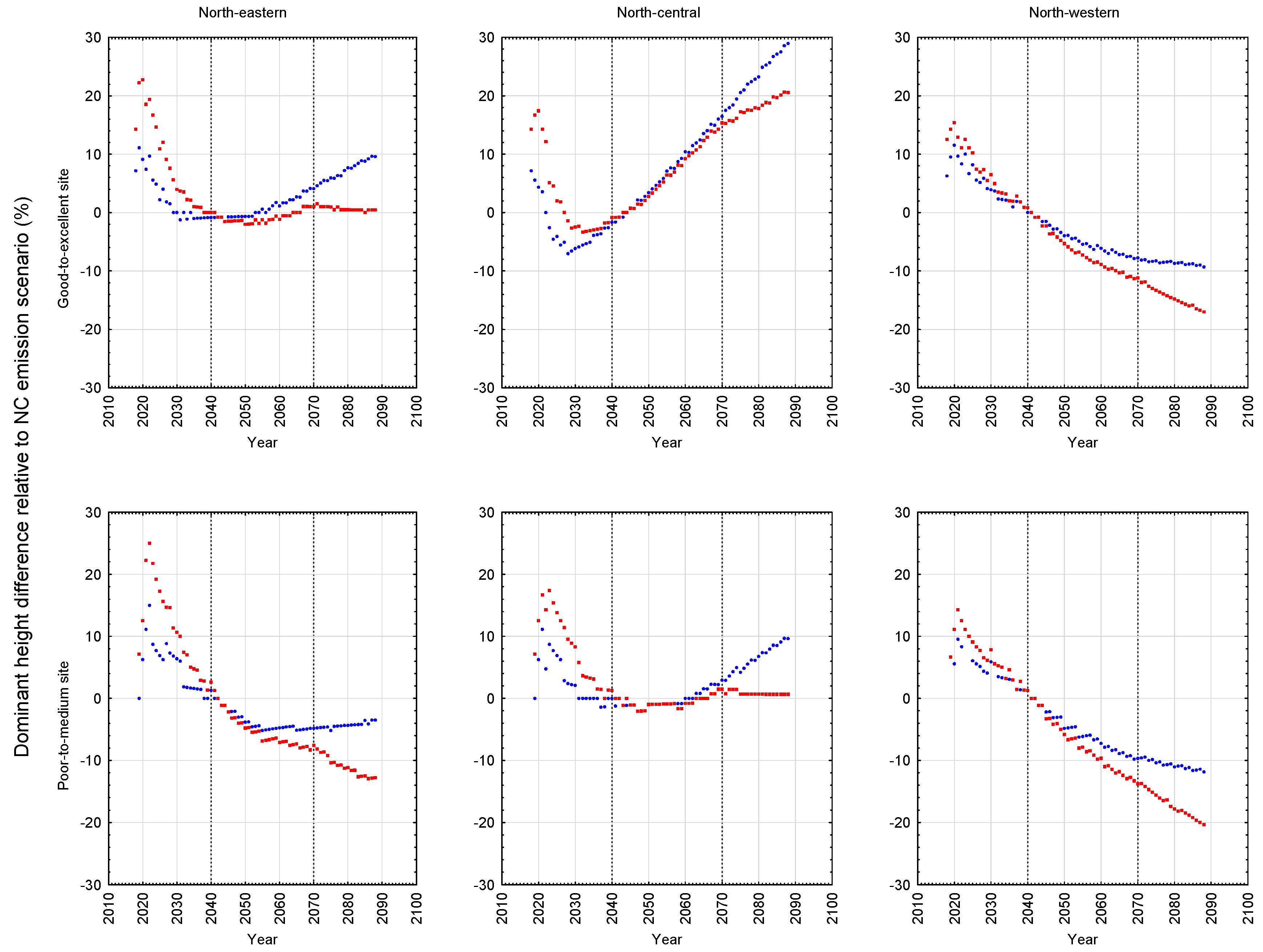
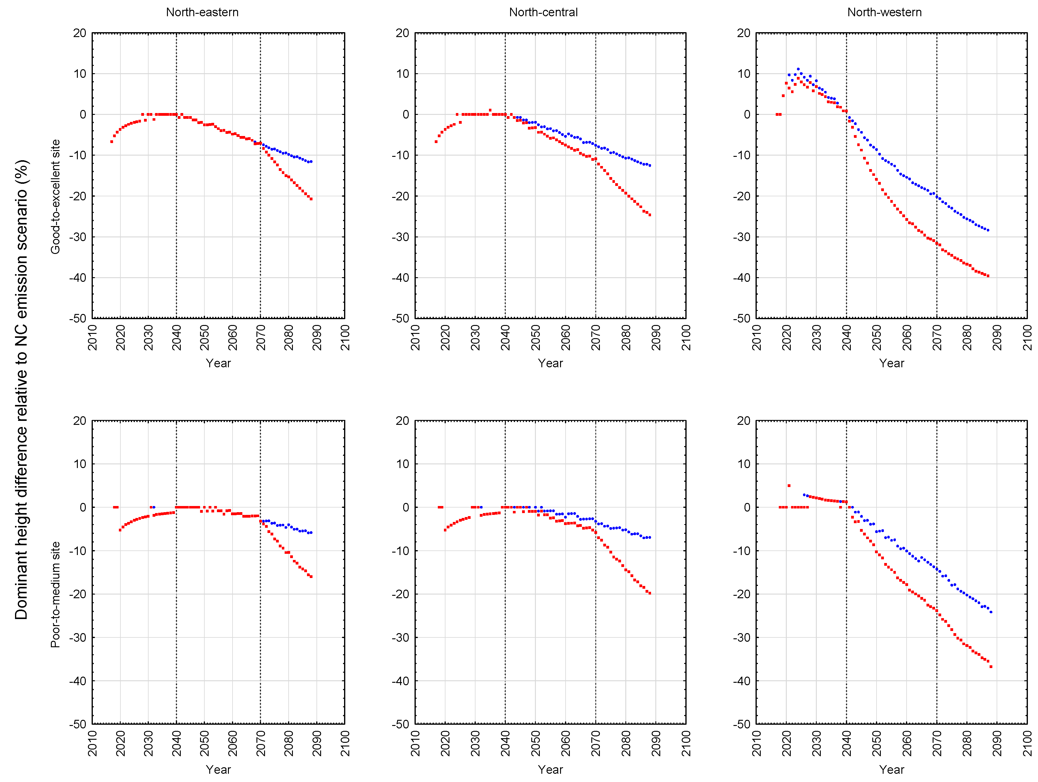
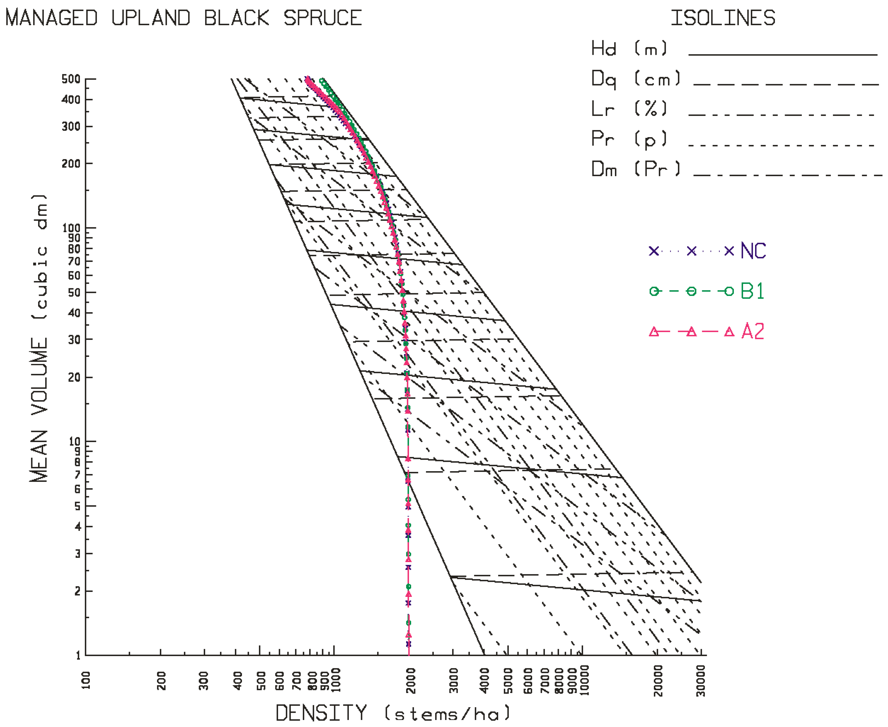
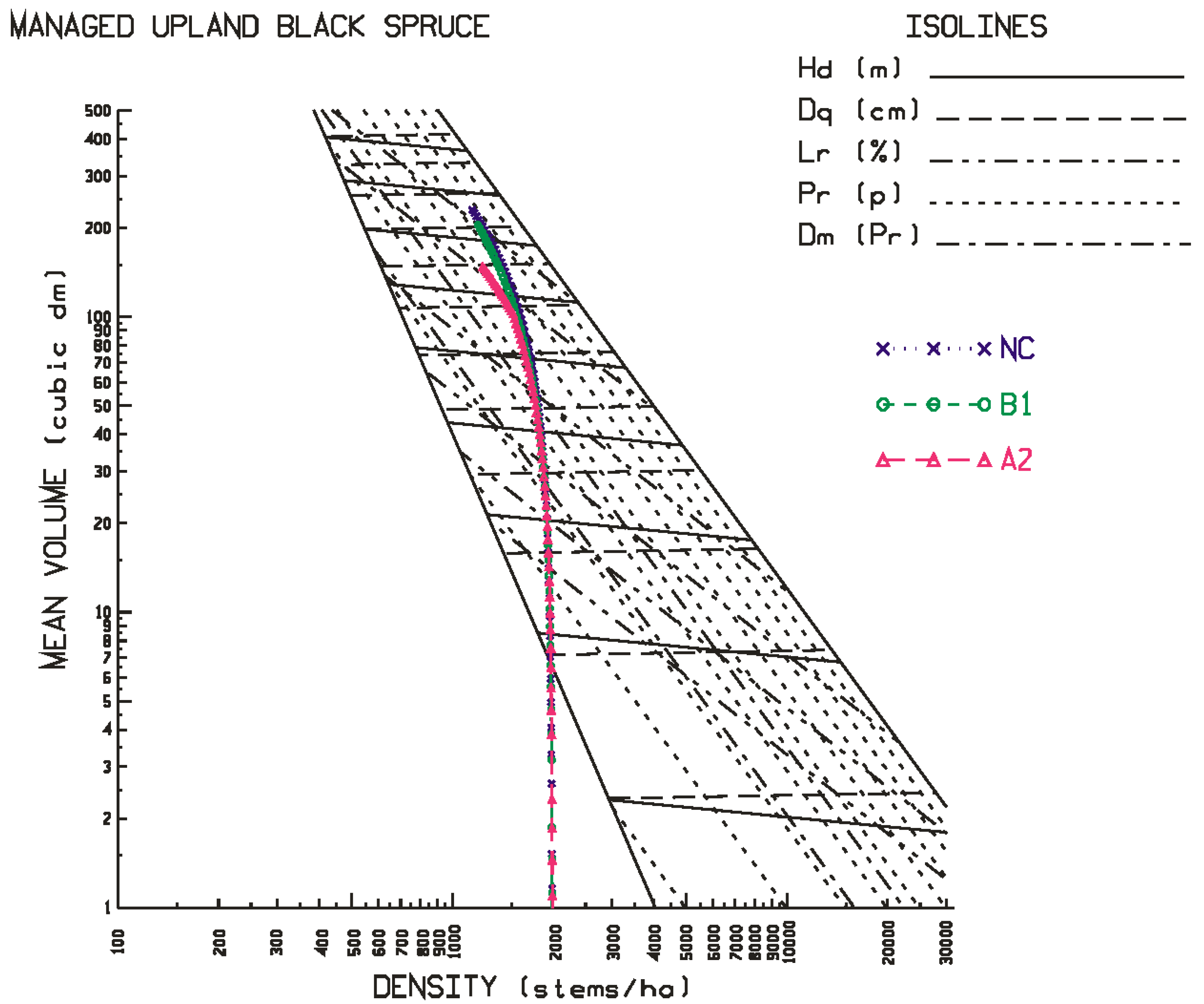
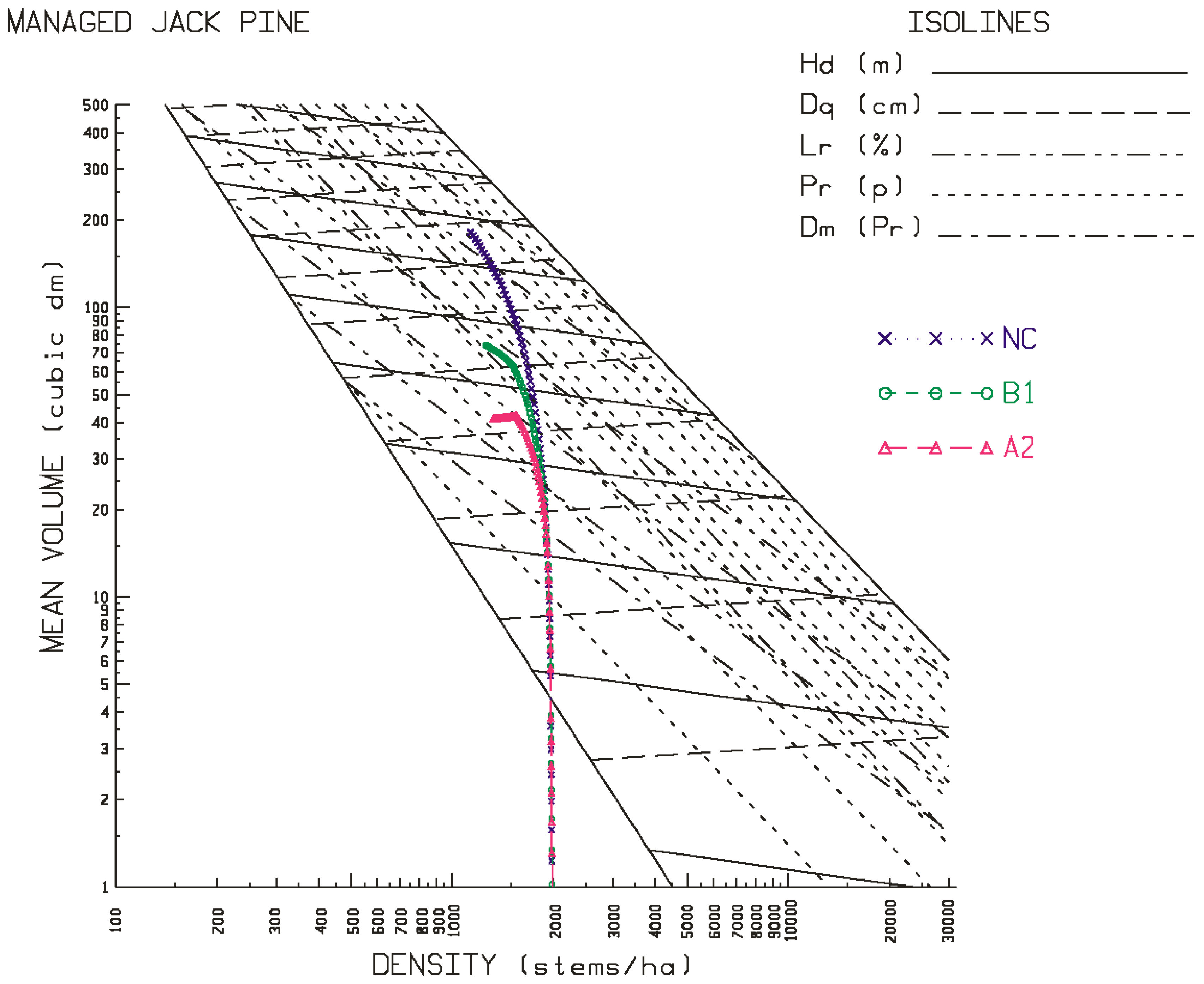
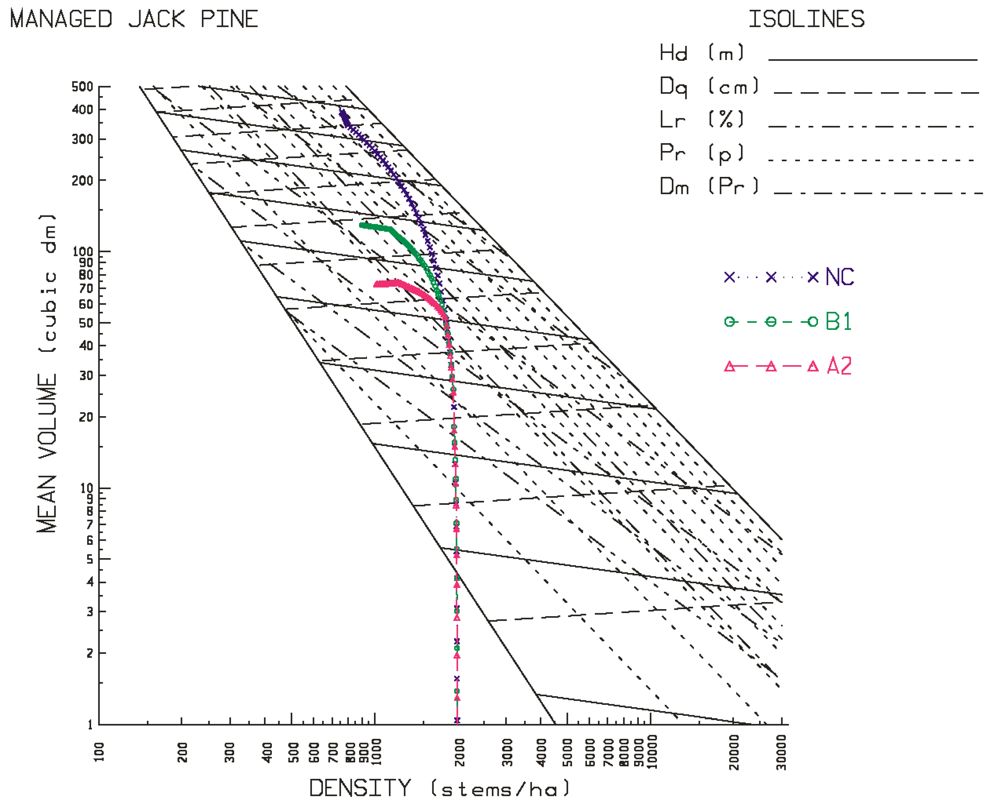
The relative differences of these predicted height development patterns for the B1 and A2 emission scenarios with respect to the NC emission scenario are graphically illustrated for black spruce plantations in Figure 5 and jack pine plantations in Figure 6 for the site qualities and locales examined in this study. As evident in the temporal patterns for black spruce, most of the positive and negative effects of climate change were initiated at the beginning of the second commitment period. Similar trends were evident for jack pine with the exception that the relative height growth reductions were greater and rate of decline accelerated during the third commitment period with respect to the A2 emission scenario. These response patterns were also consistent with the size-density trajectories illustrated in the SSDMM graphics (e.g., Figure 1 and Figure 2 for black spruce and Figure 3 and Figure 4 for jack pine) and their rotational consequences in terms of the productivity measures and performance metrics as presented in Table 3a, Table 3b and Table 3c for black spruce and Table 4a, Table 4b and Table 4c for jack pine: e.g., the greater the relative reduction in dominant height growth of the B1 and A2 scenarios (Figure 5 and Figure 6), the lower the corresponding plantation is positioned within the size-density space at rotation (Figure 1 and Figure 2 for black spruce and Figure 3 and Figure 4 for jack pine), and the greater the reduction in rotational productivity outcomes (Table 3a, Table 3b and Table 3c for black spruce and Table 4a, Table 4b and Table 4c for jack pine).

Similar approaches have been used to predict the effects of climate change for other forest tree species: e.g., lodgepole pine (Pinus contorta Douglas ex Louden) in western North America [34], and Norway spruce (Picea abies (L.) Karst.) and common beech (Fagus sylvatica L.) in central Europe [32]. The employment of the comprehensive modelling framework represented by the SSDMM conceptually parallels the previous efforts where large integrated decision-support models have been modified to account for climate change using a similar approach (e.g., FVS [8] and TASS [9]). Additionally, more elaborate biophysical models which directly account for GHG concentrations have also been developed and incorporated into stand-level decision-support systems (e.g., SILVA [7]). With respect to the modified SSDMMs presented in this study, Sharma and others [16] evaluated the significance of including additional climate variables into the biophysical height-age model specifications and concluded that adding variables such as soil-moisture related variables, would not significantly improve the explanatory performance of their models (e.g., final model forms explained over 98% of the variation in the dependent variables).

In a more general sense, these statistical quasi-causal approaches (e.g., [28]) do not afford the ability to gain insight nor understanding of the underlying ecophysiological effects of climate change on tree and stand growth processes, as do process-based models. However, these mensurational-based approaches can empirically account for climate change effects by providing a plausible range of outcomes in metrics that are of utility in forest management planning and policy formulation. As demonstrated, the decline in the rate of stand development arising from deteriorating growing conditions under climate change translates into growth reductions and productivity declines at rotation. Although survival rates were largely unaffected due to the establishment year employed (2014), plantations established in later years may very well experience failure due to climate-driven density-independent factors which could negatively affect seedling survival. Consequently, species substitution and assisted migration (population migration, range expansion, and long-distance migration [35]) are plausible silvicultural considerations when reforesting sites throughout the central portion of the Canadian Boreal Forest Region [11].

5. Conclusions

The objective of this study was to demonstrate an approach to account for climate change effects on productivity forecasts of black spruce and jack pine plantations at the stand-level by density management regime, emission scenario and commitment period, site quality, and geographic location, via the modification of existing SSDMMs. Analytically, climatic parameters as generated by a global climate model in association with a geographic-referencing climatic surface model for three commitment periods and three geographic locations under three plausible emissions scenarios, were used as input values to the biophysical-based site-specific height-age functions. The resultant functions, when integrated within the SSDMMs, enabled the estimation of climate change effects on a broad array of stand-level productivity measures. Analyzing the simulated responses of these commercially-important species, across a broad range of geographic locations and commitment periods, provided a more complete assessment of the potential range of climate change effects than have previous mensurational-based attempts (e.g., [22]). Empirically, the simulation results for the specific locations and sites examined, suggested that the predicted warmer and wetter growing seasons arising from increases in the emission of greenhouse gases and aerosols, will negatively affect the productivity of black spruce in north-eastern (poor-to-medium site qualities) and north-western Ontario, and jack pine irrespective of locale or site quality, over the next 75 years. Initially, the effects will be minimal but will increase dramatically with time as the full forcing effects of the B1 and A2 emission scenarios take effect during the later commitment periods (2041–2070 and 2071–2100 periods); with the later period eliciting much greater negative responses.

Although near-term projections using current emission patterns suggest that achieving a 2020 emission level that will limit increases in global temperature to 2 °C or less will be challenging [36], mitigation efforts are in a constant state of flux [13]. Furthermore, our scientific understanding of climate change and its effects is constantly improving and hence the certainty of current forecasts is largely unknown. Employment of an adaptive evaluation procedure consisting of annual field assessments of predicted climatic change effects in association with an iterative modelling approach, is a plausible future research pathway for tracking effects and improving projections. For example, the deployment of ground and (or) remote monitoring systems and technologies could assist in verifying current model predictions, detect and quantify new climate effects, and inform future modeling efforts. Other factors arising from climate change which were not explicitly considered in this study will obviously affect long-term productivity. These include the increased occurrence and severity of biotic (e.g., insect and disease [37]) and abiotic (e.g., wildfire [38]) impacts, increased rates of decomposition, unknown interactions between hydrological and biochemical cycles, and the CO₂ fertilization effect (e.g., [39]). Given the unknown impact of these effects on forest productivity and limitations of the statistical quasi-causal modeling approach [26], caution must be exercised when interpreting the predicted consequences of climate change.

References

1. Watkins, L. The Forest Resources of Ontario; Forest Evaluation and Standards Section; Forests Branch, Ontario Ministry of Natural Resources: Sault Ste. Marie, ON, Canada, 2011.
2. Parker, W.C.; Colombo, S.J.; Cherry, M.L.; Greifenhagen, S.; Papodopol, C.; Flannigan, M.D.; McAlpine, R.S.; Scarr, T. Third millennium forestry: What climate change might mean to forests and forest management in Ontario. For. Chron. 2000, 76, 445–463. [Google Scholar] [CrossRef]
3. Colombo, S.J.; McKenney, D.W.; Lawrence, K.M.; Gray, P.A. Climate Change Projections for Ontario: A Practical Guide for Policymakers and Planners; Climate Change Research Report CCRR-05; Applied Research and Development Branch, Ontario Ministry of Natural Resources: Peterborough, ON, Canada, 2007.
4. Gauthier, S.; Bernier, P.; Burton, P.J.; Edwards, J.; Isaac, K.; Isabel, N.; Jayen, K.; Le Goff, H.; Nelson, E.A. Climate change vulnerability and adaptation in the managed Canadian boreal forest. Environ. Rev. 2014, 22, 256–285. [Google Scholar] [CrossRef]
5. Newton, P.F. Development of an integrated decision-support model for density management within jack pine stand-types. Ecol. Model. 2009, 220, 3301–3324. [Google Scholar] [CrossRef]
6. Newton, P.F. A decision-support system for density management within upland black spruce stand-types. Environ. Model. Softw. 2012, 35, 171–187. [Google Scholar] [CrossRef]
7. Pretzsch, H. Application and evaluation of the growth simulator SILVA 2.2 for forest stands, forest estates and large regions. Forstwiss. Cent. 2002, 121, 28–51. [Google Scholar]
8. Crookston, N.L.; Rehfeldt, G.E.; Dixon, G.E.; Weiskittel, A.R. Addressing climate change in the forest vegetation simulator to assess impacts on landscape forest dynamics. For. Ecol. Manag. 2010, 260, 1198–1211. [Google Scholar] [CrossRef]
9. O’Neill, G.A.; Nigh, G. Linking population genetics and tree height growth models to predict impacts of climate change on forest production. Glob. Chang. Biol. 2011, 17, 3208–3217. [Google Scholar] [CrossRef]
10. Nakicenovic, N.; Alcamo, J.; Davis, G.; Vries, B.D.; Fenhann, J.; Gaffin, S.; Gregory, K.; Grübler, A.; Jung, T.Y.; Kram, T.; et al. IPCC Special Report on Emissions Scenarios (SRES); Intergovernmental Panel on Climate Change (IPCC); Cambridge University Press: New York, NY, USA, 2000. [Google Scholar]
11. Rowe, J.S. Forest regions of Canada; Publication No. 1300; Canadian Forestry Service, Department of Environment Government of Canada: Ottawa, ON, Canada, 1972.
12. IPCC (Intergovernmental Panel on Climate Change). Climate Change 2007: Synthesis Report; Contribution of Working Groups I, II and III to the Fourth Assessment Report of the Intergovernmental Panel on Climate Change; Intergovernmental Panel on Climate Change: Geneva, Switzerland, 2007. [Google Scholar]
13. Stocker, T.F.; Qin, D.; Plattner, G.K.; Alexander, L.V.; Allen, S.K.; Bindoff, N.L.; Bréon, F.M.; Church, J.A.; Cubasch, U.; Emori, S.; et al. Technical summary. In Climate Change 2013: The Physical Science Basis. Contribution of Working Group I to the Fifth Assessment Report of the Intergovernmental Panel on Climate Change; Stocker, T.F., Qin, D., Plattner, G.K., Tignor, M., Allen, S.K., Boschung, J., Nauels, A., Xia, Y., Bex, V., Midgley, P.M., Eds.; Cambridge University Press: Cambridge, UK; New York, NY, USA, 2013. [Google Scholar]
14. Carmean, W.H.; Niznowski, G.P.; Hazenberg, G. Polymorphic site index curves for jack pine in Nothern Ontario. For. Chron. 2001, 77, 141–150. [Google Scholar] [CrossRef]
15. Carmean, W.H.; Hazenberg, G.; Deschamps, K.C. Polymorphic site index curves for black spruce and trembling aspen in northwest Ontario. For. Chron. 2006, 82, 231–242. [Google Scholar] [CrossRef]
16. Sharma, M.; Subedi, N.; Ter-Mikaelian, M.; Parton, J. Modeling climatic effects on stand height/site index of plantation grown jack pine and black spruce trees. For. Sci. 2015, 61, 25–34. [Google Scholar] [CrossRef]
17. Environment Canada. The Third Generation Coupled Global Climate Model, Canadian Centre for Climate Modelling and Analysis. Available online: http://www.ec.gc.ca/ccmac-cccma/default.asp?n=1299529F-1 (accessed on 13 May 2016).
18. McKenney, D.; Papadopol, P.; Campbell, K.; Lawrence, K.; Hutchinson, M. Spatial Models of Canada- and North America-Wide 1971/2000 Minimum and Maximum Temperature, Total Precipitation and Derived Bioclimatic Variables; Frontline Technical Note No. 106; Great Lakes Forestry Centre, Canadian Forest Service: Sault Ste. Marie, ON, Canada, 2006.
19. Crins, W.J.; Gray, P.A.; Uhlig, P.; Wester, M.C. The Ecosystems of Ontario, Part I: Ecozones and Ecoregions; Technical Report SIB TERIMA TR-01; Inventory, Monitoring and Assessment Section; Ontario Ministry of Natural Resources: Peterborough, ON, Canada, 2009.
20. Ecoregions Working Group. Ecoclimatic Regions of Canada, First Approximation; Ecological Land Classification Series No. 23; Sustainable Development Branch, Canadian Wildlife Service, Environment Canada: Ottawa, ON, Canada, 1989.
21. Newton, P.F. Genetic worth effect models for boreal conifers and their utility when integrated into density management decision support system. Open J. For. 2015, 5, 105–115. [Google Scholar] [CrossRef]
22. Newton, P.F. Simulating site-specific effects of a changing climate on jack pine productivity using a modified variant of the CROPLANNER model. Open J. For. 2012, 2, 23–32. [Google Scholar] [CrossRef]
23. Coulombe, S.; Bernier, P.Y.; Raulier, F. Uncertainty in detecting climate change impact on the projected yield of black spruce (Picea mariana). For. Ecol. Manag. 2010, 259, 730–738. [Google Scholar] [CrossRef]
24. Girardin, M.P.; Raulier, F.; Bernier, P.Y.; Tardif, J.C. Response of tree growth to a changing climate in boreal central Canada: A comparison of empirical, process-based, and hybrid modeling approaches. Ecol. Model. 2008, 213, 209–228. [Google Scholar] [CrossRef]
25. Boisvenue, C.; Running, S.W. Impacts of climate change on natural forest productivity—Evidence since the middle of the 20th century. Glob. Chang. Biol. 2006, 12, 1–21. [Google Scholar] [CrossRef]
26. Grant, R.F.; Barr, A.G.; Black, T.A.; Iwashita, H.; Kidson, J.; McCaughey, H.; Morgenstern, K.; Murayama, S.; Nesic, Z.; Saigusa, N.; et al. Net ecosystem productivity of boreal jack pine stands regenerating from clearcutting under current and future climates. Glob. Chang. Biol. 2007, 13, 1423–1440. [Google Scholar] [CrossRef]
27. Loustau, D.; Bosc, A.; Colin, A.; Ogée, J.; Davi, H.; François, C.; Dufrêne, E.; Déqué, M.; Cloppet, E.; Arrouays, D.; et al. Modeling climate change effects on the potential production of French plains forests at the sub-regional level. Tree Physiol. 2005, 25, 813–823. [Google Scholar] [CrossRef] [PubMed]
28. Pretzsch, H. Forest Dynamics, Growth, and Yield; Springer: Berlin, Germany, 2009. [Google Scholar]
29. Myneni, R.B.; Keeling, C.D.; Tucker, C.J.; Asrar, G.; Nemani, R.R. Increased plant growth in the northern high latitudes from 1981 to 1991. Nature 1997, 386, 698–702. [Google Scholar] [CrossRef]
30. Kurz, W.A.; Dymond, C.C.; White, T.M.; Stinson, G.; Shaw, C.H.; Rampley, G.J.; Smytha, C.; Simpson, B.N.; Neilson, E.T.; Trofymow, J.A.; et al. CBM-CFS3: A model of carbon-dynamics in forestry and land-use change implementing IPCC standards. Ecol. Model. 2009, 220, 480–504. [Google Scholar] [CrossRef]
31. Shaw, C.; Chertov, O.; Komarov, A.; Bhatti, J.; Nadporozskaya, M.; Apps, M.; Bykhovets, S.; Mikhailov, A. Application of the forest ecosystem model EFIMOD 2 to jack pine along the boreal forest transect Case study. Can. J. Soil Sci. 2006, 86, 171–185. [Google Scholar] [CrossRef]
32. Albert, M.; Schmidt, M. Climate-sensitive modelling of site-productivity relationships for Norway spruce (Picea abies (L.) Karst.) and common beech (Fagus sylvatica L.). For. Ecol. Manag. 2010, 259, 739–749. [Google Scholar] [CrossRef]
33. Subedi, N.; Sharma, M. Climate-diameter growth relationships of black spruce and jack pine trees in boreal Ontario, Canada. Glob. Chang. Biol. 2013, 19, 505–516. [Google Scholar] [CrossRef] [PubMed]
34. Monserud, R.A.; Huang, S.M.; Yang, Y.Q. Predicting lodgepole pine site index from climatic parameters in Alberta. For. Chron. 2006, 82, 562–571. [Google Scholar] [CrossRef]
35. Ste-Marie, C. Adapting Sustainable Forest Management to Climate Change: A Review of Assisted Tree Migration and Its Potential Role in Adapting Sustainable Forest Management to Climate Change; Climate Change Task Force; Canadian Council of Forest Ministers: Ottawa, ON, Canada, 2014. [Google Scholar]
36. Friedlingstein, P.; Andrew, R.M.; Rogelj, J.; Peters, G.P.; Canadell, J.C.; Knutti, R.; Luderer, G.; Raupach, M.R.; Schaeffer, M.; van Vuuren, D.P.; et al. Persistent growth of CO2 emissions and implications for reaching climate targets. Nat. Geosci. 2014, 7, 709–715. [Google Scholar] [CrossRef] [Green Version]
37. Dukes, J.S.; Pontius, J.; Orwig, D.; Garnas, J.R.; Rodgers, V.L.; Brazee, N.; Cooke, B.; Theoharides, K.A.; Stange, E.E.; Harrington, R.; et al. Responses of insect pests, pathogens, and invasive plant species to climate change in the forests of northeastern North America: What can we predict? Can. J. For. Res. 2009, 39, 231–248. [Google Scholar] [CrossRef]
38. Wotton, B.M.; Nock, C.A.; Flannigan, M.D. Forest fire occurrence and climate change in Canada. Int. J. Wildland Fire 2010, 19, 253–271. [Google Scholar] [CrossRef]
39. Girardin, M.P.; Bernier, P.Y.; Raulier, F.; Tardif, J.C.; Conciatori, F.; Guo, X.J. Testing for a CO2 fertilization effect on growth of Canadian boreal forests. J. Geophys. Res. 2011, 116, 1–16. [Google Scholar] [CrossRef]
Figure 1. Temporal size-density trajectories by scenario for black spruce plantations within the context of the SSDMM graphic for poor-to-medium quality sites (SI = 8.6) within north-eastern Ontario. Graphically illustrating: (1) isolines for mean dominant height (Hd; diagonal solid lines ranging from a minimum of 4 m at the bottom of the graphic to a maximum of 20 m at the top of the graphic separated by 2 m increments), quadratic mean diameter (Dq; horizontal long dashed lines ranging from a minimum of 4 cm at the bottom of the graphic to a maximum of 26 cm at the top of the graphic separated by 2 cm increments), mean live crown ratio (Lr; diagonal lines starting at the 35% (highest placed line) then 40% and thereafter at increasing 10% increments until 80% (lowest placed line)), and relative density index (Pr; 0.1-1.0 by 0.1 intervals (short-dashed diagonal lines)); (2) crown closure line (lower diagonal solid line) and self-thinning rule at a Pr = 1.0 (upper diagonal solid line); (3) lower and upper relative density (Pr) diagonal isolines delineating the optimal density management window (Dm; 0.32 ≤ Pr ≤ 0.45). and (4) expected 75 year size-density trajectories with 1 year intervals denoted for each emission scenario (NC, B1, and A2). Source: Modified SSDMM for black spruce.
Forests 07 00223 g001
Figure 2. Temporal size-density trajectories by scenario for black spruce plantations within the context of the SSDMM graphic for good-to-excellent quality sites (SI = 12.6) within north-eastern Ontario. Note, all graphical denotations and definitions follow that given in the caption of Figure 1. Source: Modified SSDMM for black spruce.
Forests 07 00223 g002
Figure 3. Temporal size-density trajectories by scenario for jack pine plantations within the context of the SSDMM graphic for poor-to-medium quality sites (SI = 8.6) within north-western Ontario. Graphically illustrating: (1) isolines for mean dominant height (Hd; diagonal solid lines ranging from a minimum of 4 m at the bottom of the graphic to a maximum of 22 m at the top of the graphic separated by 2 m increments), quadratic mean diameter (Dq; horizontal long dashed lines ranging from a minimum of 4 cm at the bottom of the graphic to a maximum of 24 cm at the top of the graphic separated by 2 cm increments), mean live crown ratio (Lr; diagonal lines starting at the 35% (highest placed line) then 40% and thereafter at increasing 10% increments until 80% (lowest placed line)), and relative density index (Pr; 0.1-1.0 by 0.1 intervals (short-dashed diagonal lines)); (2) crown closure line (lower diagonal solid line) and self-thinning rule at a Pr = 1.0 (upper diagonal solid line); (3) lower and upper relative density (Pr) diagonal isolines delineating the optimal density management window (Dm; 0.32 ≤ Pr ≤ 0.45); and (4) expected 75 year size-density trajectories with 1 year intervals denoted for each scenario. Source: Modified SSDMM for jack pine.
Forests 07 00223 g003
Figure 4. Temporal size-density trajectories by scenario for jack pine plantations within the context of the SSDMM graphic for good-to-excellent quality sites (SI = 12.4) within north-western Ontario. Note, all graphical denotations and definitions follow that given in the caption of Figure 3. Source: Modified SSDMM for jack pine.
Forests 07 00223 g004
Figure 5. Dominant height developmental differences for black spruce plantations relative to the NC emission scenario (%) for the B1 (circle) and A2 (square) emission scenarios by site quality and locale. The vertical dotted lines denote termination of the first and second commitment periods (2040 and 2070, respectively).
Forests 07 00223 g005
Figure 6. Dominant height developmental differences for jack pine plantations relative to the NC emission scenario (%) for the B1 (circle) and A2 (square) emission scenarios by site quality and locale. The vertical dotted lines denote termination of the first and second commitment periods (2040 and 2070, respectively).
Forests 07 00223 g006