
Automating Plot-Level Stem Analysis from Terrestrial Laser Scanning


Department of Geography, University of Lethbridge, Lethbridge, AB T1K 3M4, Canada
*
Author to whom correspondence should be addressed.
Forests 2016, 7(11), 252; https://doi.org/10.3390/f7110252
Submission received: 25 August 2016
/
Revised: 8 October 2016
/
Accepted: 24 October 2016
/
Published: 28 October 2016
(This article belongs to the Special Issue Forest Ground Observations through Terrestrial Point Clouds)
Abstract
:Terrestrial laser scanning (TLS) provides an accurate means of analyzing individual tree attributes, and can be extended to plots using multiple TLS scans. However, multiple TLS scans may reduce the effectiveness of individual tree structure quantification, often due to understory occupation, mutual tree occlusion, and other influences. The procedure to delineate accurate tree attributes from plot scans involves onerous steps and automated integration is challenging in the literature. This study proposes a fully automatic approach composed of ground filtering, stem detection, and stem form extraction algorithms, with emphasis on accuracy and feasibility. The delineated attributes can be useful to analyze terrain, tree biomass and fiber quality. The automation was experimented on a mature pine plot in Finland with both single scan (SS) and multiple scans (MS) datasets. With mensuration as reference, digital terrain models (DTM), stem locations, diameters at breast height (DBHs), stem heights, and stem forms of the whole plot were extracted and validated. Results of this study were best using the multiple scans (MS) dataset, where 76% of stems were detected (n = 49). Height extraction accuracy was 0.68 (r2) and 1.7 m (RMSE), and DBH extraction accuracy was 0.97 (r2) and 0.90 cm (RMSE). Height-wise stem diameter extraction accuracy was 0.76 (r2) and 2.4 cm (RMSE).
Keywords:
terrestrial laser scanning; forestry; DTM; DBH; stem detection; stem form; automatic; plot scale; TLS; point cloud segmentation1. Introduction
Decision making in forestry is traditionally dependent on forest inventories, or specifically, the means and totals of forest characteristics within a defined area [1,2]. Decisions about habitat conservation and carbon balance are grounded by inventory attributes such as tree height, diameter at breast height (DBH), tree volume, age, and biomass [3,4,5]. Silviculture, logging, and harvesting benefit from a knowledge of stem form, fiber length, and wood density [3,6,7,8]. Ecological regulation by prescribed fire or enrichment can also be advised in light of species, canopy base height, canopy closure, and tree density [9,10,11]. Therefore, delineating inventory attributes becomes an indispensable mission in forestry.
Mammoth delineation efforts have been made, generally to conform to two purposes: maximizing delineation accuracy and minimizing manual cost. For the former purpose, in-situ surveying of individual trees is usually necessary as a reliable and accurate quantification of inventory attributes such as species, DBH, basal area, tree height, and biomass. Measurement error is subject to the surveying instrument, method, and human error. Based on a control survey, Berger et al. [12] points out that the Australian national forest inventories of conifers contains an average of 1.1% relative standard deviation in DBH measurement and 3.3% in height measurement. To fulfill the latter purpose, sampling strategies such as stratified sampling, plot sampling, and transection are adopted in practice [13]. However, sampling methods are still time-consuming to cover large-area inventory. Rice et al. [14] records the durations to survey basal area factors of 437 plots in Maine using six different sampling methods. Results show that the average surveying time for one plot amounts between approximately 150 and 2300 minutes without considering traveling time. The surrogate for large-area in-situ surveying is air photo interpretation. Since the 1950s, aerial photography and other remote sensing imagery have enabled consistent canopy attribute delineation in a timely manner [15], and have gradually become a leading method in delivering large-area inventory data. Until March, 2004, plot-based inventory from photography and satellite data occupies 93.7% of the total inventory in Canada’s National Forest Inventory [16]. The satellite- or airborne-based variables from above canopy top, on the other hand, are limited in terms of extracting below canopy [17,18,19,20,21]. Overcoming this limitation is where Terrestrial Laser Scanning (TLS) technology has great potential. A modern TLS system can densely scan sub-canopy surroundings within a few hundred meters with high accuracy [21,22]. Comparing to in-situ surveying, a stationary or mobile TLS avoids intensive manual measurement and destruction, and provides highly detailed inventory information [18,23,24,25]. In brief, TLS arises as an appropriate and efficient tool to delineate detailed inventory under canopy.
A convenient inventory service from TLS is to delineate stem form attributes. Stem form attributes, such as stem diameters and stem shape, are among the typical descriptors of stem volume and biomass [26]. Branch-free bole section, stem taper, and tree height are extrinsic indicators of wood quality attributes such as basic wood density and fiber length [20,27,28]. Earlier studies focused on obtaining gross dimensions of stem form, such as DBH and tree height [18,29,30,31]. DBH can be estimated accurately using the circle-fitting method with an approximate error under 1 cm [22,32,33]. To unveil more stem form details, more recent studies have progressed to extracting stem diameters at any height [23,29,30,34,35,36]. Aschoff et al. [34], for example, sliced tree point clouds at specified heights, and then fit circles for each slice, in order to estimate height-specific diameters. Maas et al. [30] compared the stem diameters extracted from TLS with the harvester reference, and reported an root mean square error (RMSE) of 4.7 cm. Still, these height-specific slicing methods are insufficient to represent true stem form. Kankare et al. [33] observed noncircular shapes of height slice, and pointed out the accuracy of diameter estimation is strongly impacted by the stem curve (stem medial axis). This is partly because slicing a learning stem at each height leads to oval cross sections, making a simple circle-fitting algorithm invalid. A refined method is to extract diameters that are orthogonal to the stem directions, which can be achieved by cylinder fitting of stem surface points [26,37,38,39]. Liang et al. [26] automated a robust least-square cylinder fitting method to extract stem diameters from multiple pine and spruce scans. With field measured stem form diameters as reference, an evaluation of extraction accuracy shows a mean RMSE of 1.13 cm per tree, as low as manual extraction from TLS [26]. Note that the cylinder fitting accuracy relies on a clear classification of stem points. Classifying stem points against branch and foliage points may fail in complex scenes using simple constraints such as strong surface flatness and near-vertical direction in [23,24,26,39]. Indeed, measuring upper-stem diameters with branches in the foreground is the most challenging part of stem form quantification [12]. Watt and Donoghue [40] concluded that measuring tree taper is only reliable below the canopy. Tansey et al. [41] suggested incorporating airborne laser scanning (ALS) data to mitigate the effect of crown occlusion. It is clear that stem classification in the heavy branching regions needs to be treated carefully. In addition to stem classification, three problems are confronted in delineating stem form: point occlusion, stem shape variation, and noise interference. Point occlusion breaks a continuous surface down to a mixture of narrow or wide pieces, giving rise to a zigzagging pattern of the extracted stem node and diameters [32]. Stem shape variation introduces complexity to the design of fitting models and parameters [37,42]. Noise points such as ghost points can affect the accuracy of local circle fitting [43,44]. Solutions to these problems are still in demand [45].
Stem detection is a preprocessing step of delineating stem form attributes from plot scans. Stem locations can be detected efficiently based on 2-D features of a point cloud slice at a specified height (e.g., 1.3 m). The 2-D features include angular stem width [46,47], circle fitting error [29,30,35], or convergence after Hough transformation [34,48]. Other studies extract stem locations after 3-D classification of stem points based on geometric characteristics such as flatness of a point cluster, point density, and vertical histogram [26,39,49,50,51]. The accuracy of tree detection is dependent on the number of scans [52], stem density [40], branching occlusion [53], and understory occlusion [54]. In general, 3-D stem classification is more stable than stem detection using only one slice at a certain height, because it is less affected by point occlusion at the specific height [44]. However, the existing 3-D classification methods are point-wise and require time-consuming spatial computation such as nearest neighbor search. An efficient stem detection based on 3-D geometrical features is needed. Data reduction such as DTM removal is also helpful to improve the efficiency and accuracy of stem detection [55,56].
This study proposes an automated approach to extract individual stem form from plot-scale TLS scans. We also intend to evaluate the different performances of using a single scan and multiple scans. We first test a piecewise inverse-distance-weighted (IDW) ground filtering algorithm, extract stem locations using a 3-D directional mask, segment and classify point clouds supported by region growing concept, and finally, apply a stem-shape extraction algorithm. During the process of extracting individual stem form, occlusion effect can be reduced by using neighbor-independent stem classification, stem shape variation can be modeled by circle fitting of local stem points, and noise points can be segmented apart from stem points at the step of segmentation. It is intended that these automatic methods will improve the robustness and rapidity in which TLS data can be analysed, with results of interest to the forest industry.
2. Materials Preparation
The study site is a Scott pine (Pinus sylvestris L.) plot with a stem density of 479 stem per ha in Evo, Finland (61.19° N, 25.11° E). Our study plot is among a larger set of plots acquired for the EuroSDR International TLS benchmark project: Benchmarking of Terrestrial Laser Scanning for Forestry Applications [57]. The plot was scanned using Leica HDS6100 by the Finnish Geodetic Institute (FGI) during the summer of 2014. Two TLS datasets were acquired from FGI at this site: a single scan (SS) from the plot center and multiple scans (MS) from both the center and four corners. Both datasets were trimmed to the size of 32 m × 32 m with a point resolution of 15.7 mm and a distance accuracy of ±2 mm at the distance of 25 m per plot. Validation data are field mensuration of stem location, stem DBH, and tree height, as well as offline measurement of stem form and DTM from manual or semi-automated software tools. Stem form is represented as diameters and horizontal center coordinates at each height, at 1 m height intervals up to the highest measurable height inside crown. DTM reference has a resolution of 0.2 m.
3. Methodology
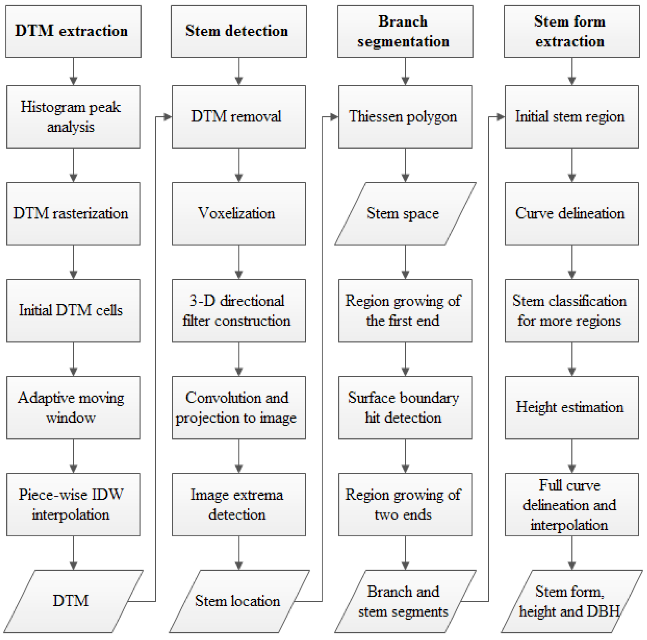
A suit of algorithms were developed in Matlab to automate the retrieval of stem attributes from point clouds without manual interference. The workflow consists of four steps: DTM extraction and removal, stem location detection and separation, branch and stem segmentation, and stem form extraction. Figure 1 illustrates a flow diagram of methods used in this study, and described in the following sections.
3.1. DTM Extraction
The extraction and removal of DTM can expedite the following step of stem detection and stem form extraction. The general approach of DTM extraction is to detect the candidate ground points and interpolate full ground points from the neighboring candidate ground points.
In forested terrain, initial separation of ground and canopy is a necessary procedure prior to fine DTM extraction [58]. An upper threshold () for DTM is needed to distinguish ground and canopy. According to [29,59], the can be estimated based on the histogram of point elevations (Figure 2). The first histogram peak () is detected when the slope of the histogram profile reduces to 0. The width of the first peak () is calculated as full width at half maximum (FWHM). The upper threshold for the DTM elevation () is defined following (1), where is the controlling parameter for adjusting . The candidate ground points are considered lower than . In this study, we set to be as large as 5, in order to incorporate all ground points as candidate ground points.
In order to extract the local lowest points, point clouds are rasterized first. Compared to raw irregular points or Triangulated Irregular Network (TIN), raster format can greatly expedite search for spatial neighbors [60]. All 3-D points () are mapped into a raster cell by normalizing the with DTM resolution (). We set to be 0.2 m. The elevation of is assigned to be a cell value. Only the lowest elevation inside the cell is kept as the cell value. Empty cells, often a result of occlusion of laser returns, are initially assigned with a positive large value (e.g., 10,000). A square moving window at an initial length of 5 cells is then applied to each cell. The selection of the initial size can be arbitrary because the initial size has little influence on the final results. The local lowest points () are thus computed as the lowest cell value inside the moving window.
The candidate ground points can be filtered using (2). Note that is the cell value of candidate ground points, and (0.5 m in this study) is the elevation tolerance in the moving window. The candidate ground point cells are used as support cells to interpolate the center cell value inside the moving window.
The ground points represented by the candidate ground points are likely to have large gaps in canopy areas. Our solution follows the concept from Zhang et al. [61] which adaptively increases moving window size to proliferate candidate ground points. The size of the moving window keeps increasing until the window covers at least candidate ground point cells. should be large enough (e.g., 10) to avoid noise cells. Our intention is to preserve the lowest elevation information and constrain abrupt elevation changes in the step of interpolation. This can be achieved by designing a robust weight function in light of [58,62]. The center cell value is set to be either unchanged or IDW neighbor values. It is determined by a piecewise function as (3), where symbol is the size of the moving window, symbol is the distance between cell (,) and cell (,), and is the final ground point value at row and column in the result raster. Only points > 0.1 m above the final ground point value are kept in the following analysis. Those points are regarded as the above-ground points.
3.2. Stem Location Extraction and Isolation
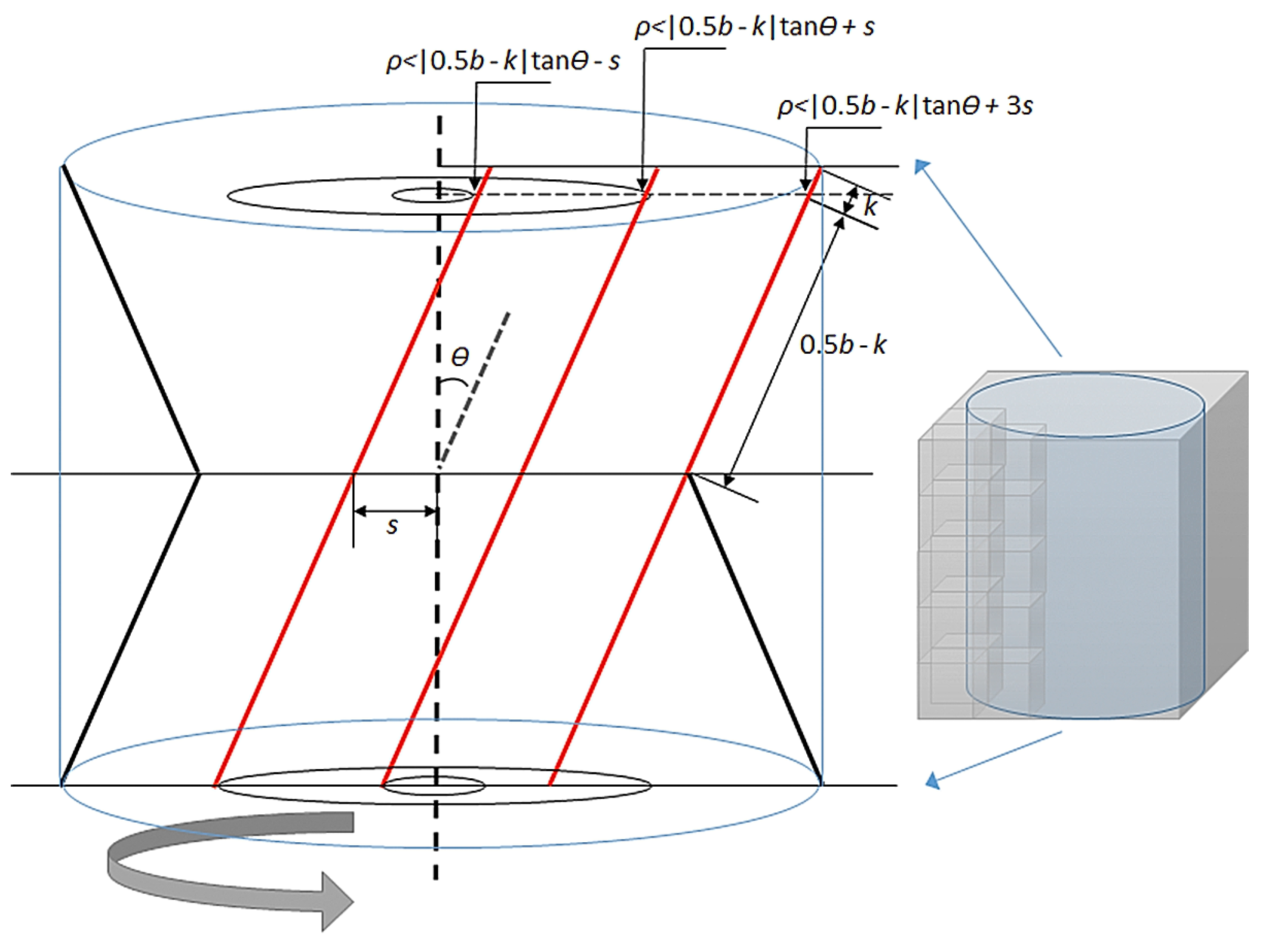
Tree stems are identified using template matching (or filter) in 3D space explained in [63]. A 3-D template is developed to detect tree stems that extend upwards from the ground surface, and have a leaning angle smaller than . First, above-ground point clouds are divided into voxels at a resolution of 0.1 × 0.1 × 0.5 m (xyz). The vertical resolution is set at 0.5 m because we expect greater horizontal than vertical heterogeneity. Each voxel is assigned the value of the point count inside the voxel, thereby representing point density. Voxels from the point clouds are multiplied respectively by a 3-D template, or what we call a 3-D directional filter in our study. The 3-D directional filter is also composed of voxels. A sum of the product of point cloud voxels and filter voxels is called convolution. It is efficient to enhance the near-vertical characteristics through 3-D convolution, by assigning “1” or any positive value “” to a filter voxel as a reward, and “−1” as a penalty. The structure and size of the filter should be designed to reward all stem points within the stem cylinder, and penalize non-stem points outside the cylinder. The mathematic description of our 3-D directional filter is shown in Figure 3. We use the parameter s to represent the horizontal radius of “” voxels (reward voxels), numerically close to horizontal stem cylinder radius. We then set the ring thickness of “−1” voxels (penalty voxels) to be s as well. The filter height is b (1 m in this study). The filter width and depth are both 0.5b tan + 2s, where is the current leaning angle. A rough estimation of s is half DBH (0.2 m in this study). The voxel representation of the filter is demonstrated on the right side of Figure 3. Overall, the directional filter is a cylinder shape filled with the penalty voxels and reward voxels. Assuming lean angle is horizontally symmetric, the reward voxels as a whole appear like a revolution geometry, which is formed by rotating the two left thickest lines (Figure 3) 360° around the vertical axis. The penalty voxels appear like another revolution geometry, formed by rotating the two right thickest lines (Figure 3) 360° around the vertical axis. The remaining filter voxels are filled with “0”. We define ρ as a voxel’s distance to the centerline, k as the voxel’s distance along the rotational line to the line’s top end. For each voxel, when ρ < |0.5b − k| tan − s or ρ > |0.5b − k| tan + 2s, the voxel value is assigned “−1”; when |0.5b − k| tan − s ≤ ρ ≤ |0.5b − k| tan + s, the voxel value is assigned ; when ρ doesn’t satisfy the above two conditions, the voxel value is kept “0”. To represent different leaning angles, five filters are created with the leaning angles of 0°, 5°, 10°, 15°, and 20°, respectively. The five filter masks are then averaged to get an overall 3-D directional filter.
This convolution step can be accelerated using the 3-D Fourier transformation. Interested readers can refer to Nixon [64] about the theory. Specifically, we calculate the 3-D Fourier form of the point cloud voxels and the 3-D Fourier form of the overall 3-D directional filter. The two Fourier forms are multiplied and the inverse Fourier form of multiplication is our convolution result. The convolution only enhances any near-vertical points within the filter size. To aggregate the enhancement for the whole stem, the 3-D convolution value in each voxel is summed again vertically, and is projected to the horizontal plane as a 2-D image. In this manner, near-vertical points are displayed as bright pixels in the 2-D image, whereas points with other spatial patterns turn to dark pixels. Only pixels with brightness greater than a threshold remain. The threshold is defined as the product of point density, sum of award voxels in the overall filter, and as well as a controllable parameter (0.5 in this study). If a remaining bright pixel has brightness greater than neighboring pixels, it is defined as a local extrema. The stem locations can be determined by searching the local extrema of the bright pixels from the 2-D image. The image coordinates are converted back to real-world coordinates by inverting the voxelization step.
The above-ground point clouds can be separated in to stem-wise occupation areas based on the detected stem locations. We define stem occupation area approximately as the Thiessen polygon around the stem location. In this study, we observed that pine stems did not move beyond 1 m horizontally from the center location. The point clouds are therefore trimmed to be within 1 m horizontal radius from the stem location, so as to reduce computing overhead. Trimming based on prior knowledge or exploratory analysis is not a necessary step, but helps improve automation efficiency.
3.3. Stem Form Extraction: Segmentation
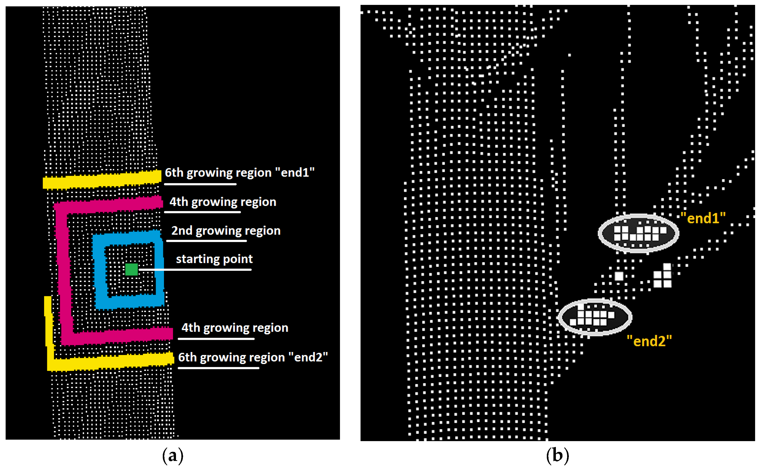
Region growing method is useful to approximate stem and branch morphology based on the geometric properties of a surface, including local connectivity and fractals, as well as the dynamics of the geometry and curvature [65,66]. An illustration of the region growing algorithm is shown in Figure 4, where the algorithm is used to segment whole point clouds into numerous cylinders without a need for initial seeds. The region growing algorithm starts from one arbitrary point as shown in Figure 4a, and incorporates its neighboring points to be the 1st grown region. In this study, the neighboring points are defined as any remaining points whose absolute coordinate differences from a growing region are smaller than . Intuitively, the neighboring points lie inside nearest cubes (size ××) from the grown region. In the same manner, the next region growing iteration incorporates neighboring points around the boundary of the 1st growing region as the 2nd growing region, which is highlighted in blue in Figure 4a. The 4th, and 6th growing regions are also highlighted in different colors. At this stage, the 6th growing region is no longer continuous. The upper side of the 6th growing region (“end 1”) is separate from the lower side of the 6th growing region (“end 2”). A visual illustration of “end 1” and “end 2” is also shown in Figure 4a. We consider the status of the 6th region growing as a “hit” of the surface boundary. The boundary “hit” condition is judged by near-zero width increment of the nth grown region. Upon the “hit” of surface boundary, the grown regions together (from 1st to 6th) exhibit a cylindrical shape. After the “hit”, the growing region (i.e., “end 1” and “end 2”) continues growing, until the width of the “end 1” or “end 2”increases by more than (0.8 in this study), or the direction of the “end 1” or “end 2”changes by more than (60° in this study). The first termination condition indicates that the growing region reached a branch or a stem portion with a width at least greater than the current width. The second termination means that the growing region reaches another branch with more than angular difference. After the current region growing is terminated, we select a new starting point from the rest of the points and repeat the above region growing, until no new points can be found from the remaining point cloud.
Figure 4a displays a simple stem point cloud, whereas Figure 4b has the more complex situation with branching bifurcation. We intend to control region growing only along the same stem/branch surface. So bifurcated branch points need to be excluded during region growing. This is realized by partitioning the nth growing region points into clusters, and only keeping the largest two clusters. The nearest distance between any two clusters should be greater than . In other words, is a gap parameter to differentiate region connectivity. In this study, is assigned to be a constant 0.01 m but can be also set as a multiple of the average point resolution, to adapt to different point cloud datasets. Here we focus on the largest two clusters. The largest cluster is assigned to be the “end 1”, and the second largest cluster to be the “end 2”, so as to limit the growing region to be on the stem surface. However, due to point occlusion, the branch may be larger than the stem, and “end 2” may thus be a branch. As such, we add a restriction that “end 2” is classified as the second largest cluster only if that cluster is located in the opposite growing direction of “end 1”. The whole segmentation algorithm and its required parameters are described in Algorithm 1. Note that our segmentation algorithm is not aimed to filter a perfect whole stem, instead, it prepares cylindrical segments for the next step of stem classification.
| Algorithm 1. Description of point cloud segmentation using region growing method. | ||
| Input: | ||
| Output: | ||
| Parameters: | , ,, | |
| 1 | ; | |
| 2 | ||
| 3 | ||
| 4 | ; ; ; | |
| 5 | ||
| 6 | ; ; | |
| 7 | ; | |
| 8 | ||
| 9 | ||
| 10 | ||
| 11 | ||
| 12 | ||
| 13 | ||
| 14 | ||
| 15 | ||
| 16 | ||
| 17 | ||
| 18 | ||
| 19 | ||
| 20 | | |
| 21 | ||
| 22 | | |
| 23 | ||
| 24 | ||
| 25 | ||
| 26 | | |
| 27 | ||
| 28 | ||
3.4. Stem Form Extraction: Classification
Grown region with the most points is selected to initiate stem classification. The first principle component of the principle component analysis (PCA) for the stem region is chosen as an overall stem direction. The initial stem points are then perpendicularly projected to the stem direction to create their projected lengths along the stem direction. The stem points are separated into slices by splitting the projected lengths at equal intervals of 0.2 m. The purpose of slicing at equal intervals is merely to conform to validation data format. Each slice is projected along the stem direction into a plane. A circle-fit algorithm which minimizes the geometric error using least square [67] is adopted to find the circle center and radius from the projected points. As a result, the form of the initial part of stem is delineated by a sequence of the circle centers (stem nodes), circle radii (node radii), and circle directions (node directions).
More regions need to be classified as part of the stem. One condition is set to satisfy: the region points shall fall inside a cylinder. The centerline of the cylinder starts from the closest node and is collinear with that node direction. The radius of the cylinder is the closest node radius. A concentric buffer cylinder is used to search new regions. The radius of the buffer cylinder is equal to the node radius timed by . Here is a user-defined ratio parameter indicating the degree of tolerance to the buffer cylinder radius (1.3 in this study). Priority is given to closer and larger regions. After a new region is classified as part of the stem region each time, the stem form is re-delineated using the circle fitting algorithm. Upper-stem and occluded regions may have few points to support circle fitting. Neighboring regions are then searched until sufficient points (e.g., 200) are found. The whole classification process terminates when no regions are found to fall inside the cylinder.
Upper-stem occlusion is common in plot-level TLS scans. Due to upper-stem occlusion, the extracted stem form contains only visible components, yet the full stem form should extend continuously from the bottom to the tree top. Tree height is determined in our algorithm as the vertical distance between the highest and lowest points inside each isolated stem point cloud. The previous delineated stem form is linearly interpolated to zero radius at the tree top. Deficient stems with height lower than 2 m, or diameter smaller than 5 cm are removed from the final results of stem form extraction.
3.5. Validation
DTM, stem detection, stem DBH, stem height, and stem form can be validated using the reference data. The DTM error is defined by the mean distance between extracted DTM points and corresponding nearest points in reference DTM. We only focus on how well the extracted locations from TLS matched the surveyed locations. Our detection rate is defined as the number of detected stems within a tolerable distance to the closest reference stems, divided by the total number of reference stems. The tolerable distance is set to be 0.5 m, so as to allow for possible surveying error of reference locations. This automated calculation of detection rate produces the same results as manual matching in our study. The reference stem nodes manually extracted from each stem point clouds by FGI are organized as 3-D coordinates of the stem nodes following a height sequence of 0.65 m, 1.3 m, 2 m, 3 m, 4 m, and so on. Automatically extracted stem nodes are also interpolated to the same height sequence in order to match the reference stem nodes. The match of our nodes and reference nodes is based on the nearest neighbor search from the reference nodes. For each detected stem curve, RMSE of diameters, and r2 of diameters between the extracted nodes and the reference nodes are investigated.
The parameters needed in all steps are displayed in Table 1. The parameter values in the right column can be used as default values in different TLS datasets. Other values were attempted in a few trials and errors, and extraction results did not vary greatly, because the algorithms allow reasonable variations of scanning conditions, point density, and stem geometry. For example, if or is set to smaller values (larger than minimum point resolution), the point clouds will be segmented into smaller pieces, but the following classification step will still recognize stem points based on . Parameter tuning is not suggested for the purpose of improving accuracy. We fixed the parameter values as in the right column of Table 1 throughout the processing of both SS and MS datasets.
4. Results and Discussion
4.1. DTM Extraction
Both SS and MS point clouds from plot-1 were processed fully automatically based on the a-priori parameters without referring to any mensuration data.
The 3-D points of the extracted DTM from the MS dataset are shown in Figure 5. The point color is rendered by the distance between extracted DTM point and its nearest point in reference DTM. Points with the distance <0.2 m are shown in blue, 0.2–0.4 m green, 0.4–0.5 m yellow, and >0.5 m red. As expected, our DTM extraction algorithm preserves local low points and smoothens upper points. Local low points are not smoothened, so distance is high in the area of pits and bulges. The upper land on the bottom right of Figure 5 also shows high distance value, because ground points are inadequate in that vegetated area to support accurate interpolation. For plot-1, average DTM error is 0.16 m (SS) and 0.10 m (MS), respectively. The DTM errors are reasonable, for both the reference and the produced DTMs have a resolution of 0.2 m.
4.2. Stem Location Extraction and Isolation
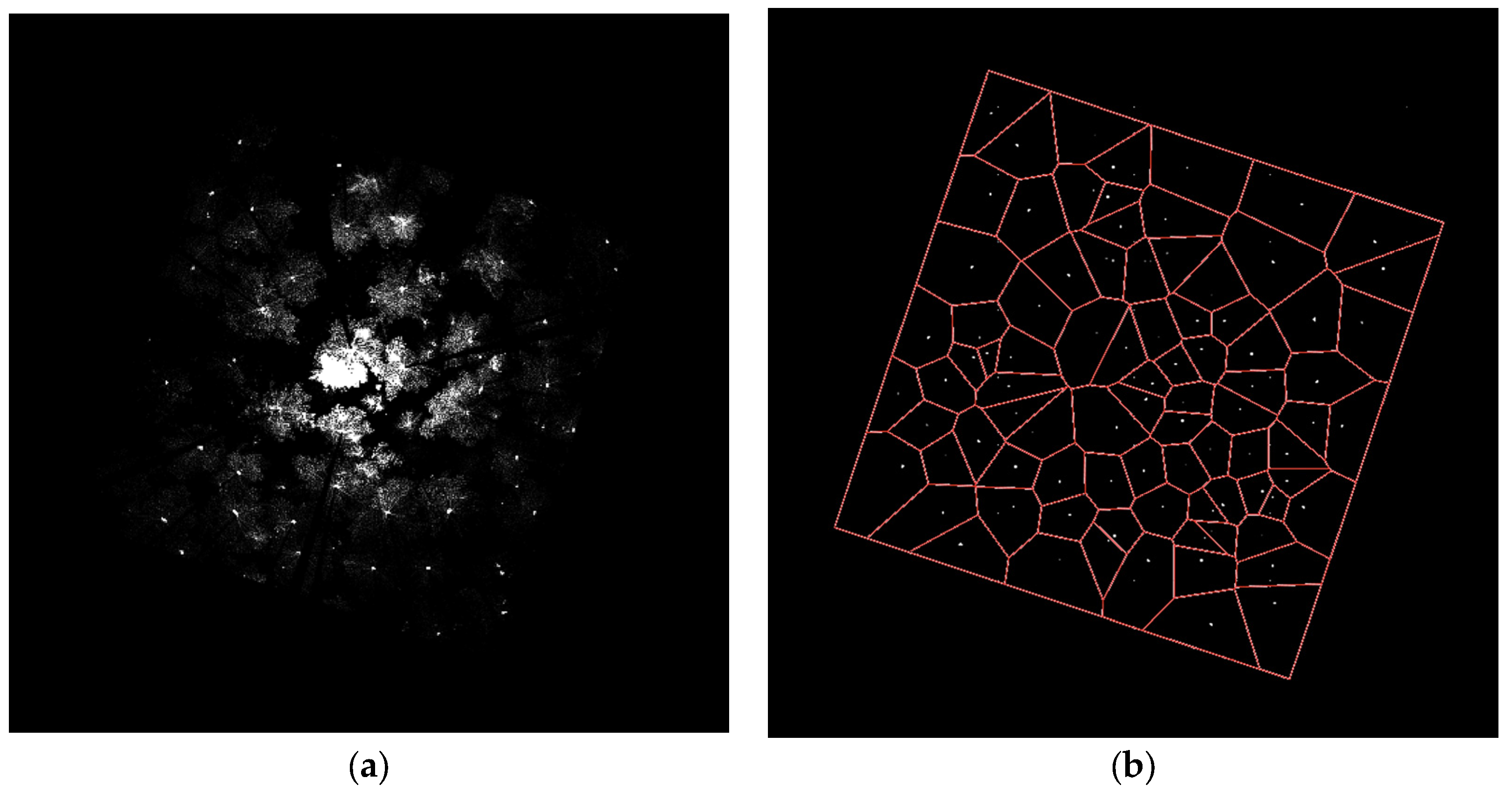
The projected 2-D image of 3-D directional filter convolution using MS dataset is shown in Figure 6b, offering comparison to the projected image without applying the directional filter in Figure 6a. It can be seen that irrelevant matters such as branch and foliage are cleared using our directional filter in Figure 6b. The pixel brightness stays consistently high near the likely stem locations and drops drastically further away. The brightness change (or sharpness) is controlled by the 3-D filter size parameter s and filter value . A high degree of sharpness produces speckled effect of the 2-D image and leads to over-detection of stem locations. To avoid high sharpness, s is suggested to approximate or exceed the size of stem target and stay below 2. In addition, high sharpness can be mitigated by increasing the maximum-allowed leaning angle . A large leaning angle (>40°), however, causes a risk of detecting oblique branches.
Also in Figure 6b, Thiessen polygons are shown as lines surrounding each extracted stem location. Among the detected stems from filter convolution, deficient stems were further discarded in the stem classification step. As a result, a total of 50 (SS) and 58 (MS) stems were detected, where 40 (SS) and 41 (MS) stems could match to reference stems (49 stems). Therefore, a few trees exist in TLS scans but are not sampled in the reference data. This coincides with the finding from Liang and Hyyppä [38] that around 10% of reference stems do not show in their SS dataset. The detection rates are 81.6% (SS) and 75.5% (MS). Our detection rates are satisfactory, considering Brolly [44]’s summary of nine papers that detection rates are between 22%–94% (SS), and 52%–100% (MS). The detection rate from SS alone is also competitive, in comparison to the common range of 68%–90% from SS [68]. It is not absolute though, for detection rate relies on plot conditions such as tree species, stem density, age, and elevation. For example, detection rates of four different species with over 40 trees in Liang and Hyyppä [38] range from 81% to 100%.
4.3. Stem Form Extraction
A visualisation of the stem curve extraction is shown in Figure 7 for a single tree. The stem points are heavily shaded by branches and leaves at the height above 10 m (Figure 7a). The loss of stem points in upper stems above 10 m is also reported in Henning and Radtke [23], and above 7.8 m reported in Bienert et al. [53]. The extraction algorithm used is able to identify the stem shape and taper through the canopy (Figure 7c) by segmenting branches (Figure 7b). Optimal region growing automation ideally requires the avoidance of a-priori estimates of stem or branch radius. A number of existing branch reconstruction studies use a predefined sphere as an initial guess of radius [69,70,71]. The classified stem reaches a height of 14.8 m, 67% of field measured height. Heavy occlusion above that height prevents our stem classification algorithm from detecting further stem surfaces. In general, the average proportion of our classified stem height reaches 64% (SS) and 74% (MS), greater than the average proportion of FGI’s software measured stem height 62% (SS) and 61% (MS). Stem diameter narrowing in the crown is another bottleneck of stem classification from branch clumps. A potential solution is to sacrifice time efficiency in order to gain classification accuracy. This could be, for example, finer region growing in terms of smaller and , or greater classification tolerance in terms of larger . Figure 7d plots the shape and radius of the extracted curve nodes. Visually, the overall curve shape is smooth. The occlusion of the crown introduces biases in the node direction above 12 m and radius above 6 m.
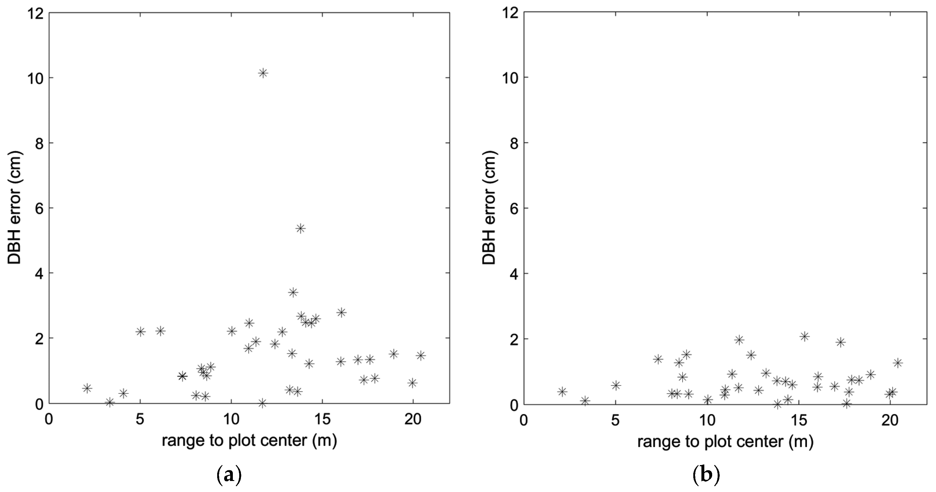
Correspondence between TLS detected stem DBH, height, and form (for those identified within 0.5 m of the reference stems) and reference is provided in Table 2. According to Liang et al. [26]’s accuracy assessment of over five studies about stem attribute extraction, DBH RMSE ranges between 0.82–9.17cm (mean: 3.8 cm), and stem diameter RMSE between 1.13–7.0 cm (mean: 3.9 cm). Our DBH and stem diameter results from MS show improvement over the average at 0.9 cm RMSE, yet results from SS are less satisfactory at 2.4 cm RMSE. The difference of DBH RMSE 1.5 cm represents 6.5% of the mean reference DBH. Here, we define “error” as the absolute difference between measured and extracted. A right-tailed two-sample t-test of DBH error comparing SS and MS shows a p-value of 0.0008 at the 5% significance level, and the same test of height error has a p-value of 0.13 at the 5% significance level. It can be concluded that DBH error from SS is significantly greater than from MS and height error from SS is not. The detailed disparity between measured and extracted DBHs can be seen in Figure 8a,b. Systematic underestimation error can be found from Figure 8a where 67.5% of extracted DBHs from SS and 94.6% from MS are smaller than the reference. It is believed that the systematic error and bias are likely due to the circle-fitting algorithm and field measurement uncertainty. The measured and extracted heights are compared in Figure 8c,d. The leading error is presented by two obvious outliers that are far from the dashed regression line in both figures. The outliers show errors greater than 5 m. We visually examined the corresponding stems and found crown tops were actually overlaid by several higher crowns from neighboring trees. At such, tree crown overlapping contributes much of the error. The distance to scanner is plotted against DBH error (SS and MS) in Figure 9. From Figure 9a, it is clear that the largest DBH errors (>5 cm) from SS correspond to a distance greater than 10 m to the plot center. Indeed, with the increase of distance to plot center, stem surface points become thinner and more scattered [72], and therefore challenge DBH extractions. In contrast, extracting DBH from MS is less affected by distance to plot center (Figure 9b), owing to additional corner scans.
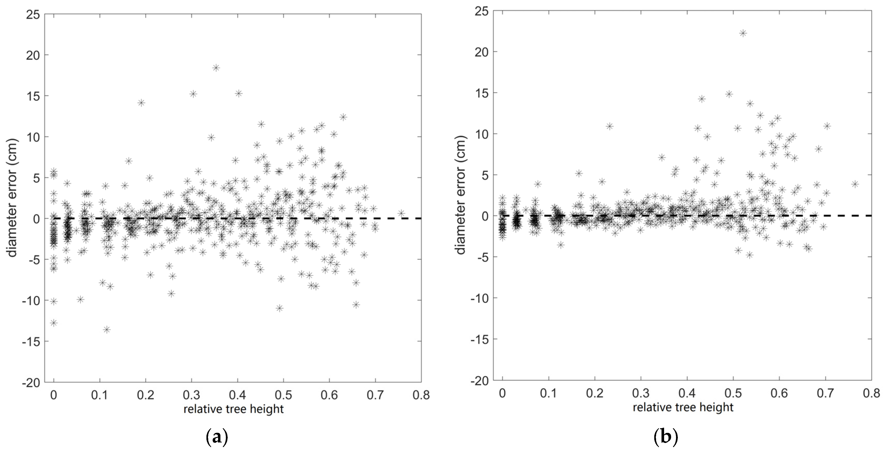
Extracting full stem diameters is more challenging than extracting DBH. The increased difficulty is clear in the mean RMSEs of extracted stem diameters (SS: 3.2 cm, MS: 2.4 cm) in Table 2 compared to that of DBH (SS: 2.4 cm, MS: 0.9 cm). The average RMSEs of extracted diameters are 3.6 cm (SS) and 3.1 cm (MS) above half tree height, contributing 65.4% and 73.3% to total RMSEs, respectively. The relationship between diameter extraction errors and relative tree heights is illustrated in Figure 10. Outliers are mostly distributed near the ground and above 40% height. It is clear that more diameters are underestimated from SS (Figure 10a) than from MS (Figure 10b). Trying different circle-fitting algorithm may overcome this problem.
4.4. Time Efficiency
In the process of stem form extraction, searching for the neighboring points is accelerated by a voxel indexing method. The voxel indexing method first groups the points into voxels and any nearby voxels are then searched directly by the spatial index. This method reduces the computation and storage cost of iterative point cloud subdivision in the octree method. Partitioning of the growing region into clusters is also facilitated by the voxel indexing method. In our test, the overall computation time is reduced to half by applying the voxel indexing method.
Our overall processing time for the plot-1 using an Intel i7 2 GHz with 8 GB memory are 27 min (SS) and 2 h 28 min (MS), respectively. The processing time for MS is distributed approximately in Table 3. Note that processing time varies with the tree geometry, point number, scan quality, and computer specification. The number of points are 23,568,575 (SS) and 111,065,193 (MS). The point cloud files are 0.5 GB (SS) and 2.5 GB (MS) and isolated stem files had a median of 1 MB (SS) and 10 MB (MS), respectively. Table 3 illustrates that the time complexity of our algorithm is highly proportional to the point number, which is partly because our algorithms limit nonlinear traversal of point clouds. A countable processing time is essential to an unsupervised, ceaseless, and achievable product line of plot-size inventory. Foresters can rehearse processing smaller point clouds, determine desired point size and resolution, and then arrange a favorable processing timeline. Only a limited number of studies share information about processing time. Aschoff and Spiecker [31] reported that their algorithms allocate 16.2 second per million points (sppm) to DTM creation, 10.8 sppm to tree recognition, but a large 865 sppm to noise reduction and export, based on a 2.0 GHz CPU. Bienert et al. [29] provided sppm statistics for three SS plots and one MS plots using Intel Xeon CPU (2.4 GHz) with 1.0 GB RAM. Their algorithm of DTM filtering, segmentation and classification has around 240 sppm (SS) and 180 sppm (MS), and their algorithm of stem form extraction has 15–22 sppm (SS) and 23 sppm (MS), respectively. In comparison, our algorithms exhibit more stable sppm between SS and MS.
5. Conclusions
This study presents a new methodology for the automated extraction of tree locations, complex DBH cross sections and detectable stem heights within a plot with single and multiple TLS scan lines. The study uses automated methods to (a) filter and retain ground returns and high resolution variability of the ground surface using an automated, piece-wise interpolation function; (b) identify stem locations via rapid matching of 3-D shapes within point clouds in entire 3-D space instead of focusing on predefined slices or point-wise principal components analysis (PCA) described previously in the literature [29,30,34,48]; and (c) applying an automated stem form extraction methodology for all identified trees within the plot such that issues associated with complex stem shape and point occlusion due to canopy interception of laser pulses are addressed. Although numerous steps are required to perform the analysis, the integration of these methods can be applied to answer numerous questions about canopy attributes that would otherwise require greater user intervention and processing time. For example, our segmentation algorithm can provide branch segments as a preliminary input to the cylinder fitting step in most branch reconstruction algorithms [70,73,74,75,76,77]. Differentiating branch segments is also an essential step to isolate overlapping trees [69,78]. Our stem detection algorithm can also aid the process of multi-scan co-registration [23].
While this study may not provide the most accurate results compared with Liang et al. [26], the automation of steps for complete plot-level assessment will reduce time spent in the field and more manually intensive TLS-based extraction methods [42,79]. Algorithm versatility is also an aim of improvement. As Côté et al. [73] pointed out, current TLS measurement still faces the problem of object occlusion, multi-scan oversampling, wind sway, and tree component identification. Solving these problems entirely is indeed a long run.
Acknowledgments
The authors would like to express their gratitude to Xinlian Liang, Harri Kaartinen, and Juha Hyyppä who kindly provided the TLS scans and mensuration data for this study. The data were eventually collected for the EuroSDR International TLS benchmark project, which is financially supported by the Finnish Academy projects “Centre of Excellence in Laser Scanning Research (CoE-LaSR) (272195) and European Community’s Seventh Framework Programme” ([FP7/2007–2013]) under grant agreement No. 606971. Chris Hopkinson acknowledges research funding from the Campus Alberta Innovates Program (CAIP) and NSERC Discovery Grants Program.
Author Contributions
Z.X. designed the algorithms and wrote the manuscript; C.H. supervised the study and introduced the datasets; C.H. and L.C. revised the manuscript.
Conflicts of Interest
The authors declare no conflict of interest. The founding sponsors had no role in the design of the study; in the collection, analyses, or interpretation of data; in the writing of the manuscript, and in the decision to publish the results.
References
- Penman, J.; Gytarsky, M.; Hiraishi, T.; Krug, T.; Kruger, D.; Pipatti, R.; Buendia, L.; Miwa, K.; Ngara, T.; Tanabe, K. Good Practice Guidance for Land Use, Land-Use Change and Forestry; Institute for Global Environmental Strategies IGES: Kanagawa, Japan, 2003; Available online: http://hdl.handle.net/123456789/6871 (Accessed on 07 July 2016).
- Kangas, A.; Maltamo, M. Forest Inventory: Methodology and Applications; Springer Science & Business Media: Berlin, Germany, 2006; Volume 10. [Google Scholar]
- Luther, J.E.; Skinner, R.; Fournier, R.A.; Van Lier, O.R.; Bowers, W.W.; Coté, J.-F.; Hopkinson, C.; Moulton, T. Predicting wood quantity and quality attributes of balsam fir and black spruce using airborne laser scanner data. Forestry 2013. [Google Scholar] [CrossRef]
- Coops, N.C.; Tompaski, P.; Nijland, W.; Rickbeil, G.J.M.; Nielsen, S.E.; Bater, C.W.; Stadt, J.J. A forest structure habitat index based on airborne laser scanning data. Ecol. Indic. 2016, 67, 346–357. [Google Scholar] [CrossRef]
- Chen, J.M.; Ju, W.; Cihlar, J.; Price, D.; Liu, J.; Chen, W.; Pan, J.; Black, A.; Barr, A. Spatial distribution of carbon sources and sinks in Canada’s forests. Tellus B 2003, 55, 622–641. [Google Scholar] [CrossRef]
- Peuhkurinen, J.; Maltamo, M.; Malinen, J.; Pitkänen, J.; Packalén, P. Preharvest measurement of marked stands using airborne laser scanning. For. Sci. 2007, 53, 653–661. [Google Scholar]
- Kankare, V.; Holopainen, M.; Vastaranta, M.; Puttonen, E.; Yu, X.; Hyyppä, J.; Vaaja, M.; Hyyppä, H.; Alho, P. Individual tree biomass estimation using terrestrial laser scanning. ISPRS J. Photogramm. Remote Sens. 2013, 75, 64–75. [Google Scholar] [CrossRef]
- Blanchette, D.; Fournier, R.A.; Luther, J.E.; Cote, J.-F. Predicting wood fiber attributes using local-scale metrics from terrestrial lidar data: A case study of Newfoundland conifer species. For. Ecol. Manag. 2015, 347, 116–129. [Google Scholar] [CrossRef]
- Jennings, S.; Brown, N.; Sheil, D. Assessing forest canopies and understorey illumination: Canopy closure, canopy cover and other measures. Forestry 1999, 72, 59–74. [Google Scholar] [CrossRef]
- Peterson, D.W.; Reich, P.B. Prescribed fire in oak savanna: Fire frequency effects on stand structure and dynamics. Ecol. Appl. 2001, 11, 914–927. [Google Scholar] [CrossRef]
- Agee, J.K.; Skinner, C.N. Basic principles of forest fuel reduction treatments. For. Ecol. Manag. 2005, 211, 83–96. [Google Scholar] [CrossRef]
- Berger, A.; Gschwantner, T.; McRoberts, R.E.; Schadauer, K. Effects of measurement errors on individual tree stem volume estimates for the austrian national forest inventory. For. Sci. 2014, 60, 14–24. [Google Scholar] [CrossRef]
- Schreuder, H.T.; Wood, G.B.; Gregoire, T.G. Sampling Methods for Multiresource Forest Inventory; John Wiley & Sons: Hoboken, NJ, USA, 1993. [Google Scholar]
- Rice, B.; Weiskittel, A.R.; Wagner, R.G. Efficiency of alternative forest inventory methods in partially harvested stands. Eur. J. For. Res. 2014, 133, 261–272. [Google Scholar] [CrossRef]
- Wulder, M. Optical remote-sensing techniques for the assessment of forest inventory and biophysical parameters. Prog. Phys. Geogr. 1998, 22, 449–476. [Google Scholar] [CrossRef]
- Gillis, M.; Omule, A.; Brierley, T. Monitoring Canada’s forests: The national forest inventory. For. Chron. 2005, 81, 214–221. [Google Scholar] [CrossRef]
- Chasmer, L.; Hopkinson, C.; Treitz, P. Investigating laser pulse penetration through a conifer canopy by integrating airborne and terrestrial lidar. Can. J. Remote Sens. 2006, 32, 116–125. [Google Scholar] [CrossRef]
- Hopkinson, C.; Chasmer, L.; Young-Pow, C.; Treitz, P. Assessing forest metrics with a ground-based scanning lidar. Can. J. For. Res. 2004, 34, 573–583. [Google Scholar] [CrossRef]
- Lovell, J.L.; Jupp, D.L.B.; Culvenor, D.S.; Coops, N.C. Using airborne and ground-based ranging lidar to measure canopy structure in australian forests. Can. J. Remote Sens. 2003, 29, 607–622. [Google Scholar] [CrossRef]
- Van Leeuwen, M.; Hilker, T.; Coops, N.C.; Frazer, G.; Wulder, M.A.; Newnham, G.J.; Culvenor, D.S. Assessment of standing wood and fiber quality using ground and airborne laser scanning: A review. For. Ecol. Manag. 2011, 261, 1467–1478. [Google Scholar] [CrossRef]
- Hilker, T.; Van Leeuwen, M.; Coops, N.C.; Wulder, M.A.; Newnham, G.J.; Jupp, D.L.; Culvenor, D.S. Comparing canopy metrics derived from terrestrial and airborne laser scanning in a douglas-fir dominated forest stand. Trees 2010, 24, 819–832. [Google Scholar] [CrossRef]
- Dassot, M.; Constant, T.; Fournier, M. The use of terrestrial lidar technology in forest science: Application fields, benefits and challenges. Ann. For Sci. 2011, 68, 959–974. [Google Scholar] [CrossRef]
- Henning, J.G.; Radtke, P.J. Detailed stem measurements of standing trees from ground-based scanning lidar. For. Sci. 2006, 52, 67–80. [Google Scholar]
- Liang, X.; Litkey, P.; Hyyppä, J.; Kaartinen, H.; Kukko, A.; Holopainen, M. Automatic plot-wise tree location mapping using single-scan terrestrial laser scanning. Photogramm. J. Finl. 2011, 22, 37–48. [Google Scholar]
- Rutzinger, M.; Pratihast, A.K.; Oude Elberink, S.J.; Vosselman, G. Tree modelling from mobile laser scanning data-sets. Photogramm. Rec. 2011, 26, 361–372. [Google Scholar] [CrossRef]
- Liang, X.; Kankare, V.; Yu, X.; Hyyppä, J.; Holopainen, M. Automated stem curve measurement using terrestrial laser scanning. IEEE Trans. Geosci. Remote Sens. 2014, 52, 1739–1748. [Google Scholar] [CrossRef]
- Kankare, V.; Joensuu, M.; Vauhkonen, J.; Holopainen, M.; Tanhuanpää, T.; Vastaranta, M.; Hyyppä, J.; Hyyppä, H.; Alho, P.; Rikala, J. Estimation of the timber quality of scots pine with terrestrial laser scanning. Forests 2014, 5, 1879–1895. [Google Scholar] [CrossRef]
- Kretschmer, U.; Kirchner, N.; Morhart, C.; Spiecker, H. A new approach to assessing tree stem quality characteristics using terrestrial laser scans. Silva Fenn. 2013, 47, 14. [Google Scholar] [CrossRef]
- Bienert, A.; Scheller, S.; Keane, E.; Mullooly, G.; Mohan, F. Application of terrestrial laser scanners for the determination of forest inventory parameters. Int. Arch. Photogramm. Remote Sens. Spat. Inf. Sci. 2006, 36(part 5). [Google Scholar]
- Maas, H.G.; Bienert, A.; Scheller, S.; Keane, E. Automatic forest inventory parameter determination from terrestrial laser scanner data. Int. J. Remote Sens. 2008, 29, 1579–1593. [Google Scholar] [CrossRef]
- Aschoff, T.; Spiecker, H. Algorithms for the automatic detection of trees in laser scanner data. Int. Arch. Photogramm. Remote Sens. Spat. Inf. Sci. 2004, 36, W2. [Google Scholar]
- Pueschel, P.; Newnham, G.; Rock, G.; Udelhoven, T.; Werner, W.; Hill, J. The influence of scan mode and circle fitting on tree stem detection, stem diameter and volume extraction from terrestrial laser scans. ISPRS J. Photogramm. Remote Sens. 2013, 77, 44–56. [Google Scholar] [CrossRef]
- Kankare, V.; Holopainen, M.; Vastaranta, M.; Puttonen, E.; Yu, X.; Hyyppä, J.; Vaaja, M.; Hyyppä, H.; Alho, P. Individual tree biomass estimation using terrestrial laser scanning. ISPRS J. Photogramm. Remote Sens. 2013, 75, 64–75. [Google Scholar] [CrossRef]
- Aschoff, T.; Thies, M.; Spiecker, H. Describing forest stands using terrestrial laser-scanning. Int. Arch. Photogramm. Remote Sens. Spat. Inf. Sci. 2004, 35, 237–241. [Google Scholar]
- Pueschel, P. The influence of scanner parameters on the extraction of tree metrics from faro photon 120 terrestrial laser scans. ISPRS J. Photogramm. Remote Sens. 2013, 78, 58–68. [Google Scholar] [CrossRef]
- Srinivasan, S.; Popescu, S.C.; Eriksson, M.; Sheridan, R.D.; Ku, N.-W. Terrestrial laser scanning as an effective tool to retrieve tree level height, crown width, and stem diameter. Remote Sens. 2015, 7, 1877–1896. [Google Scholar] [CrossRef]
- Pfeifer, N.; Winterhalder, D. Modelling of tree cross sections from terrestrial laser scanning data with free-form curves. Int. Arch. Photogramm. Remote Sens. Spat. Inf. Sci. 2004, 36, W2. [Google Scholar]
- Liang, X.; Hyyppä, J. Automatic stem mapping by merging several terrestrial laser scans at the feature and decision levels. Sensors 2013, 13, 1614–1634. [Google Scholar] [CrossRef] [PubMed]
- Liang, X.; Litkey, P.; Hyyppa, J.; Kaartinen, H.; Vastaranta, M.; Holopainen, M. Automatic stem mapping using single-scan terrestrial laser scanning. IEEE Trans. Geosci. Remote Sens. 2012, 50, 661–670. [Google Scholar] [CrossRef]
- Watt, P.; Donoghue, D. Measuring forest structure with terrestrial laser scanning. Int. J. Remote Sens. 2005, 26, 1437–1446. [Google Scholar] [CrossRef]
- Tansey, K.; Selmes, N.; Anstee, A.; Tate, N.; Denniss, A. Estimating tree and stand variables in a corsican pine woodland from terrestrial laser scanner data. Int. J. Remote Sens. 2009, 30, 5195–5209. [Google Scholar] [CrossRef]
- Dassot, M.; Colin, A.; Santenoise, P.; Fournier, M.; Constant, T. Terrestrial laser scanning for measuring the solid wood volume, including branches, of adult standing trees in the forest environment. Comput. Electron. Agric. 2012, 89, 86–93. [Google Scholar] [CrossRef]
- Huang, H.; Li, Z.; Gong, P.; Cheng, X.; Clinton, N.; Cao, C.; Ni, W.; Wang, L. Automated methods for measuring dbh and tree heights with a commercial scanning lidar. Photogramm. Eng. Remote Sens. 2011, 77, 219–227. [Google Scholar] [CrossRef]
- Brolly, G.B. Locating and Parameter Retrieval of Individual Trees from Terrestrial Laser Scanner Data. Ph.D. Thesis, University of West Hungary, Sopron, Hungary, 2013; p. 104. Available online: http://ilex.efe. hu/PhD/emk/brollygabor/disszertacio. pdf (accessed on 30 January 2016). [Google Scholar]
- Liang, X.; Kankare, V.; Hyyppä, J.; Wang, Y.; Kukko, A.; Haggrén, H.; Yu, X.; Kaartinen, H.; Jaakkola, A.; Guan, F.; et al. Terrestrial laser scanning in forest inventories. ISPRS J. Photogramm. Remote Sens. 2016, 115, 63–77. [Google Scholar] [CrossRef]
- Strahler, A.H.; Jupp, D.L.B.; Woodcock, C.E.; Schaaf, C.B.; Yao, T.; Zhao, F.; Yang, X.; Lovell, J.; Culvenor, D.; Newnham, G.; et al. Retrieval of forest structural parameters using a ground-based lidar instrument (echidna®). Can. J. Remote Sens. 2008, 34, S426–S440. [Google Scholar] [CrossRef]
- Lovell, J.; Jupp, D.; Newnham, G.; Culvenor, D. Measuring tree stem diameters using intensity profiles from ground-based scanning lidar from a fixed viewpoint. ISPRS J. Photogramm. Remote Sens. 2011, 66, 46–55. [Google Scholar] [CrossRef]
- Schilling, A.; Schmidt, A.; Maas, H.-G. Automatic tree detection and diameter estimation in terrestrial laser scanner point clouds. In Proceedings of the 16th Computer Vision Winter Workshop, Mitterberg, Austria, 2–4 February 2011; pp. 75–83.
- Wezyk, P.; Koziol, K.; Glista, M.; Pierzchalski, M. Terrestrial laser scanning versus traditional forest inventory: First results from the polish forests. In Proceedings of the ISPRS Workshop ‘Laser Scanning 2007 and SilviLaser 2007’, Espoo, Finland, 12 September 2007–14 September 2007; pp. 12–14.
- Lefsky, M.A.; Harding, D.; Cohen, W.B.; Parker, G.; Shugart, H.H. Surface lidar remote sensing of basal area and biomass in deciduous forests of eastern maryland, USA. Remote Sens. Environ. 1999, 67, 83–98. [Google Scholar] [CrossRef]
- Huang, H.; Gong, P.; Cheng, X.; Clinton, N.; Cao, C.; Ni, W.; Li, Z.; Wang, L. Forest structural parameter extraction using terrestrial LiDAR. In Proceedings of American Geophysical Union Fall Meeting, San Francisco, CA, USA, 15–19 September 2008.
- Thies, M.; Spiecker, H. Evaluation and future prospects of terrestrial laser scanning for standardized forest inventories. Forest 2004, 2, 1. [Google Scholar]
- Bienert, A.; Scheller, S.; Keane, E.; Mohan, F.; Nugent, C. Tree detection and diameter estimations by analysis of forest terrestrial laserscanner point clouds. In Proceedings of the ISPRS Workshop ‘Laser Scanning 2007 and SilviLaser 2007’, Espoo, Finland, 12–14 September 2007; pp. 50–55.
- Ducey, M.J.; Astrup, R. Adjusting for nondetection in forest inventories derived from terrestrial laser scanning. Can. J. Remote Sens. 2013, 39, 410–425. [Google Scholar]
- Litkey, P.; Puttonen, E.; Liang, X. Comparison of point cloud data reduction methods in single-scan TLS for finding tree stems in forest. In Proceedings of SilviLaser, Hobart, Australia, 16–19 October 2011.
- Yang, X.; Strahler, A.H.; Schaaf, C.B.; Jupp, D.L.B.; Yao, T.; Zhao, F.; Wang, Z.; Culvenor, D.S.; Newnham, G.J.; Lovell, J.L.; et al. Three-dimensional forest reconstruction and structural parameter retrievals using a terrestrial full-waveform lidar instrument (Echidna®). Remote Sens. Environ. 2013, 135, 36–51. [Google Scholar] [CrossRef]
- Hyyppa, J.; Liang, X. Project Benchmarking on Terrestrial Laser Scanning for forestry Applications. Available online: http://www.eurosdr.net/research/project/project-benchmarking-terrestrial-laser-scanning-forestry-applications (accessed on 20 September 2015).
- Kobler, A.; Pfeifer, N.; Ogrinc, P.; Todorovski, L.; Oštir, K.; Džeroski, S. Repetitive interpolation: A robust algorithm for dtm generation from aerial laser scanner data in forested terrain. Remote Sens. Environ. 2007, 108, 9–23. [Google Scholar] [CrossRef]
- Douillard, B.; Underwood, J.; Kuntz, N.; Vlaskine, V.; Quadros, A.; Morton, P.; Frenkel, A. On the segmentation of 3d lidar point clouds. In Proceedings of the 2011 IEEE International Conference Robotics and Automation (ICRA), Shanghai, China, 9–13 May 2011; pp. 2798–2805.
- Meng, X.; Currit, N.; Zhao, K. Ground filtering algorithms for airborne LiDAR data: A review of critical issues. Remote Sens. 2010, 2, 833. [Google Scholar] [CrossRef]
- Zhang, K.; Chen, S.-C.; Whitman, D.; Shyu, M.-L.; Yan, J.; Zhang, C. A progressive morphological filter for removing nonground measurements from airborne lidar data. IEEE Trans. Geosci. Remote Sens. 2003, 41, 872–882. [Google Scholar] [CrossRef]
- Kraus, K.; Pfeifer, N. Determination of terrain models in wooded areas with airborne laser scanner data. ISPRS J. Photogramm. Remote Sens. 1998, 53, 193–203. [Google Scholar] [CrossRef]
- Brunelli, R.; Poggiot, T. Template matching: Matched spatial filters and beyond. Pattern Recognit. 1997, 30, 751–768. [Google Scholar] [CrossRef]
- Nixon, M. Feature Extraction & Image Processing; Academic Press: Pittsburgh, Pennsylvania, PA, USA, 2008. [Google Scholar]
- Masutani, Y.; Masamune, K.; Dohi, T. Region-growing based feature extraction algorithm for tree-like objects. In Proceedings of the 4th International Conference Visualization in Biomedical Computing, vbc’96 Hamburg, Germany, 22–25 September 1996; Höhne, K.H., Kikinis, R., Eds.; Springer: Berlin, Germany, 1996; pp. 159–171. [Google Scholar]
- Roggero, M. Object segmentation with region growing and principal component analysis. Int. Arch. Photogramm. Remote Sens. Spat. Inf. Sci. 2002, 34, 289–294. [Google Scholar]
- Gander, W.; Golub, G.H.; Strebel, R. Least-squares fitting of circles and ellipses. BIT Numer. Math. 1994, 34, 558–578. [Google Scholar] [CrossRef]
- Liang, X.; Hyyppä, J.; Kukko, A.; Kaartinen, H.; Jaakkola, A.; Yu, X. The use of a mobile laser scanning system for mapping large forest plots. IEEE Geosci. Remote Sens. Lett. 2014, 11, 1504–1508. [Google Scholar] [CrossRef]
- Raumonen, P.; Casella, E.; Calders, K.; Murphy, S.; Åkerblom, M.; Kaasalainen, M. Massive-scale tree modelling from TLS data. ISPRS Ann. Photogramm. Remote Sens. Spat. Inf. Sci. 2015, 2, 189. [Google Scholar] [CrossRef]
- Hackenberg, J.; Morhart, C.; Sheppard, J.; Spiecker, H.; Disney, M. Highly accurate tree models derived from terrestrial laser scan data: A method description. Forests 2014, 5, 1069–1105. [Google Scholar] [CrossRef]
- Hackenberg, J.; Wassenberg, M.; Spiecker, H.; Sun, D. Non destructive method for biomass prediction combining TLS derived tree volume and wood density. Forests 2015, 6, 1274–1300. [Google Scholar] [CrossRef]
- Litkey, P.; Liang, X.; Kaartinen, H.; Hyyppä, J.; Kukko, A.; Holopainen, M.; Hill, R.; Rosette, J.; Suárez, J. Single-scan TLS methods for forest parameter retrieval. In Proceedings of SilviLaser 2008, 8th international conference on LiDAR applications in forest assessment and inventory, Heriot-Watt University, Edinburgh, UK, 17–19 September 2008; pp. 295–304.
- Côté, J.-F.; Fournier, R.A.; Egli, R. An architectural model of trees to estimate forest structural attributes using terrestrial LiDAR. Environ. Model. Softw. 2011, 26, 761–777. [Google Scholar] [CrossRef]
- Livny, Y.; Yan, F.; Olson, M.; Chen, B.; Zhang, H.; El-Sana, J. Automatic Reconstruction of Tree Skeletal Structures from Point Clouds; ACM Transactions on Graphics (TOG); ACM: New York, NY, USA, 2010; p. 151. [Google Scholar]
- Newnham, G.J.; Armston, J.D.; Calders, K.; Disney, M.I.; Lovell, J.L.; Schaaf, C.B.; Strahler, A.H.; Danson, F.M. Terrestrial laser scanning for plot-scale forest measurement. Curr. For. Rep. 2015, 1, 239–251. [Google Scholar] [CrossRef]
- Raumonen, P.; Kaasalainen, M.; Åkerblom, M.; Kaasalainen, S.; Kaartinen, H.; Vastaranta, M.; Holopainen, M.; Disney, M.; Lewis, P. Fast automatic precision tree models from terrestrial laser scanner data. Remote Sens. 2013, 5, 491–520. [Google Scholar] [CrossRef]
- Schilling, A.; Maas, H. Automatic reconstruction of skeletal structures from TLS forest scenes. ISPRS Ann. Photogramm. Remote Sens. Spat. Inf. Sci. 2014, 2, 321. [Google Scholar] [CrossRef]
- Yang, B.; Dai, W.; Dong, Z.; Liu, Y. Automatic forest mapping at individual tree levels from terrestrial laser scanning point clouds with a hierarchical minimum cut method. Remote Sens. 2016, 8, 372. [Google Scholar] [CrossRef]
- Eysn, L.; Pfeifer, N.; Ressl, C.; Hollaus, M.; Grafl, A.; Morsdorf, F. A practical approach for extracting tree models in forest environments based on equirectangular projections of terrestrial laser scans. Remote Sens. 2013, 5, 5424–5448. [Google Scholar] [CrossRef]
Figure 1.
Flow-diagram overview of methods used to automatically extract plot-level tree stem attributes. DTM: digital terrain models; IDW: inverse distance weighted; DBH: diameter at breast height.
Figure 1.
Flow-diagram overview of methods used to automatically extract plot-level tree stem attributes. DTM: digital terrain models; IDW: inverse distance weighted; DBH: diameter at breast height.

Figure 2.
Histogram filtering for DTM region. Triangles represent local maximum values of histogram profile. In this example, DTM is found to be lower than 2 m in elevation, which can be estimated based on the width of first histogram peak.
Figure 2.
Histogram filtering for DTM region. Triangles represent local maximum values of histogram profile. In this example, DTM is found to be lower than 2 m in elevation, which can be estimated based on the width of first histogram peak.
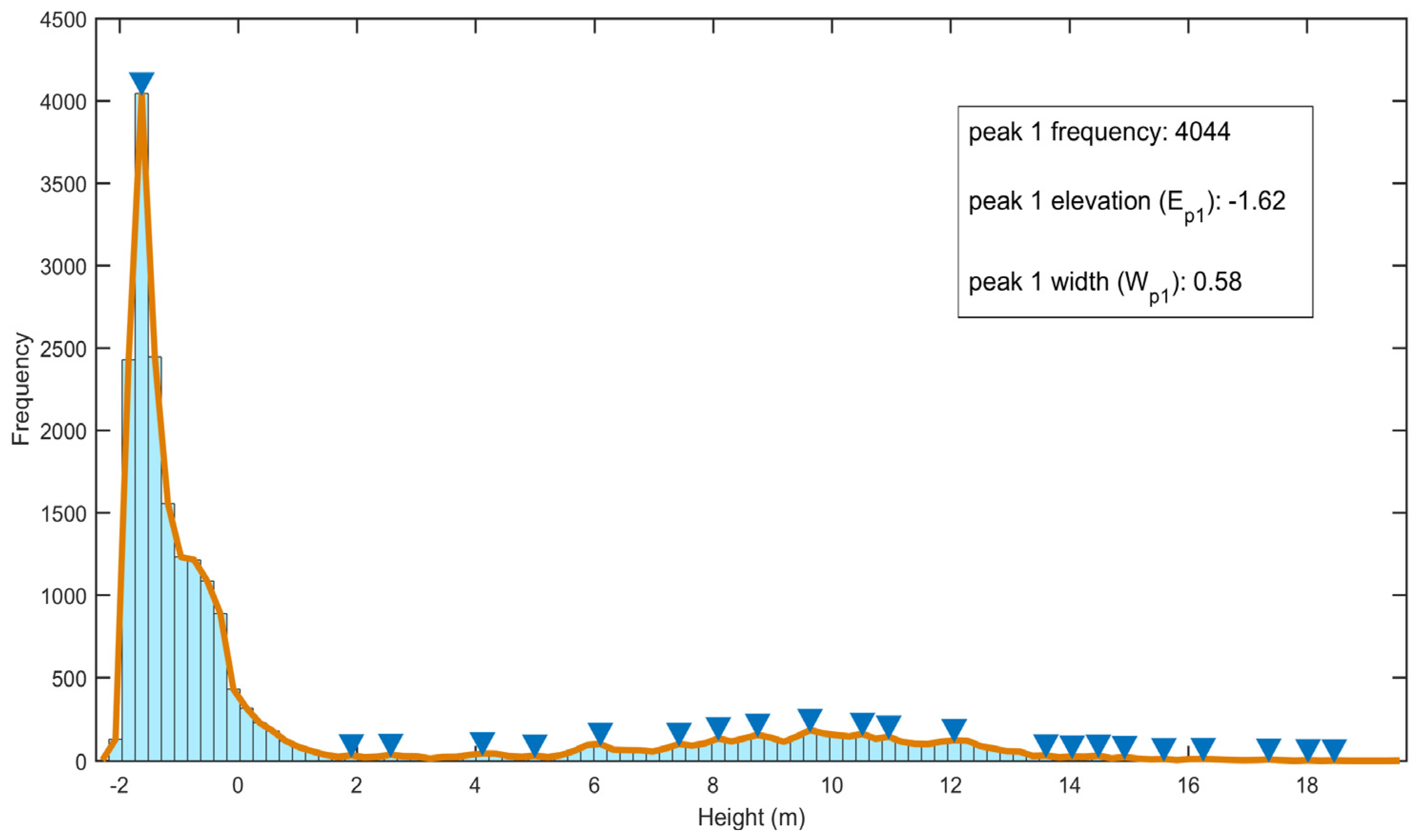
Figure 3.
3-D directional filter: a cube composed of voxels in the right; Mathematic expressions about the filter geometry and structure are noted aside.
Figure 3.
3-D directional filter: a cube composed of voxels in the right; Mathematic expressions about the filter geometry and structure are noted aside.

Figure 4.
Region growing example. (a) The starting, 2nd, 4th, and 6th growing regions colored in green, blue, pink, and yellow, respectively; (b) “end 1” and “end 2” (circled) recognized from a growing region with four clusters.
Figure 4.
Region growing example. (a) The starting, 2nd, 4th, and 6th growing regions colored in green, blue, pink, and yellow, respectively; (b) “end 1” and “end 2” (circled) recognized from a growing region with four clusters.

Figure 5.
DTM 3-D points extracted from the plot-1 multiple scans (MS) dataset. Point distance between extracted DTM and reference DTM is rendered using color legend on the right. A scale bar is placed at lower right corner.
Figure 5.
DTM 3-D points extracted from the plot-1 multiple scans (MS) dataset. Point distance between extracted DTM and reference DTM is rendered using color legend on the right. A scale bar is placed at lower right corner.
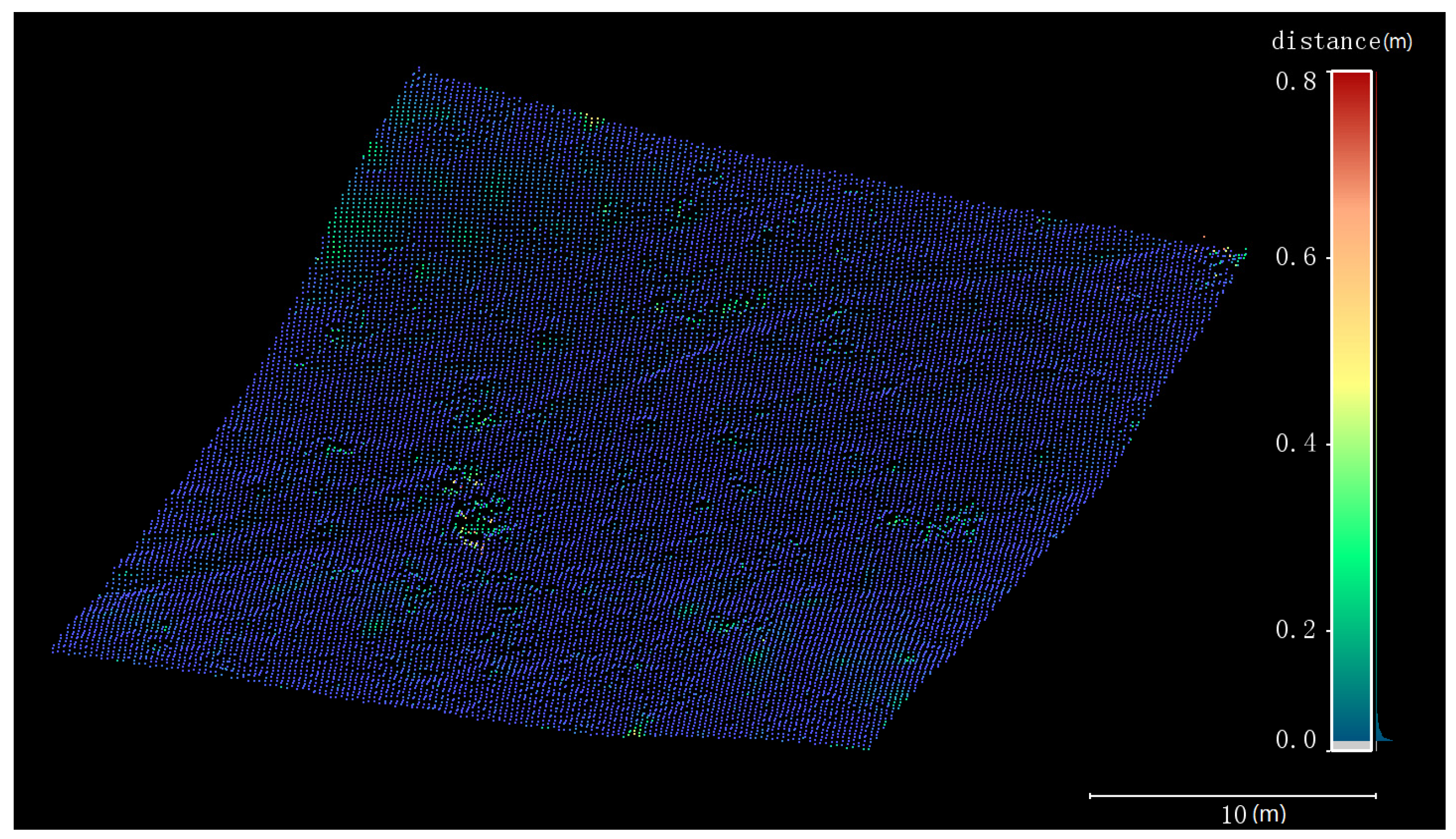
Figure 6.
Stem location detection. (a) 2-D image directly projected from point cloud voxels as a comparison; (b) 2-D image projected from the convolution of 3-D directional filter and point cloud voxels, with Thiessen polygons around the extracted locations.
Figure 6.
Stem location detection. (a) 2-D image directly projected from point cloud voxels as a comparison; (b) 2-D image projected from the convolution of 3-D directional filter and point cloud voxels, with Thiessen polygons around the extracted locations.

Figure 7.
Automation outcomes for tree No.23 from plot-1 MS. (a) raw isolated point clouds, colored by point intensity; (b) segmentation of the point clouds within 1 m horizontal distance to the stem location, colored by the segment random identity numbers; (c) a vertical section cutting tree in half, with branches in blue and classified stem in white; (d) stem radius and stem curve, represented by colored stem node circles and red connection line of stem nodes, respectively. The results are shown in local Cartesian coordinate system with plot center as the origin.
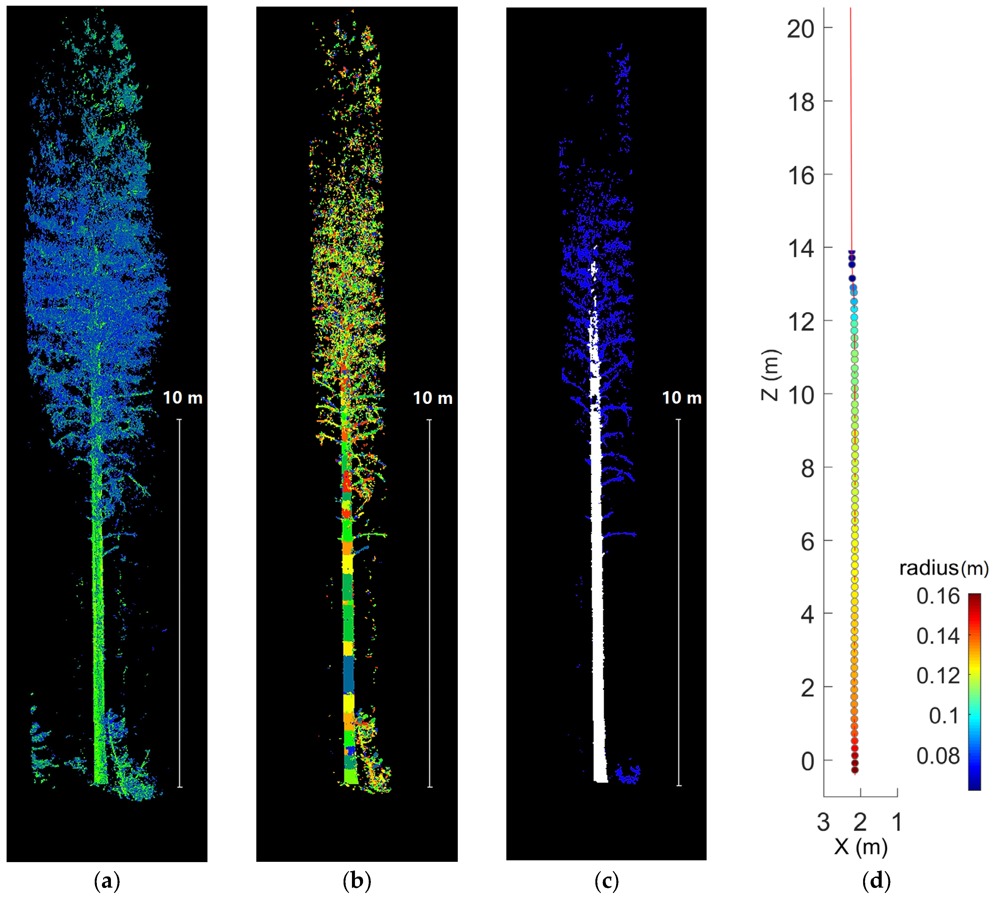
Figure 8.
Scatter plot between the measured and the extracted: (a) DBH from single scan (SS); (b) DBH from MS; (c) height from SS; (d) height from MS.
Figure 8.
Scatter plot between the measured and the extracted: (a) DBH from single scan (SS); (b) DBH from MS; (c) height from SS; (d) height from MS.
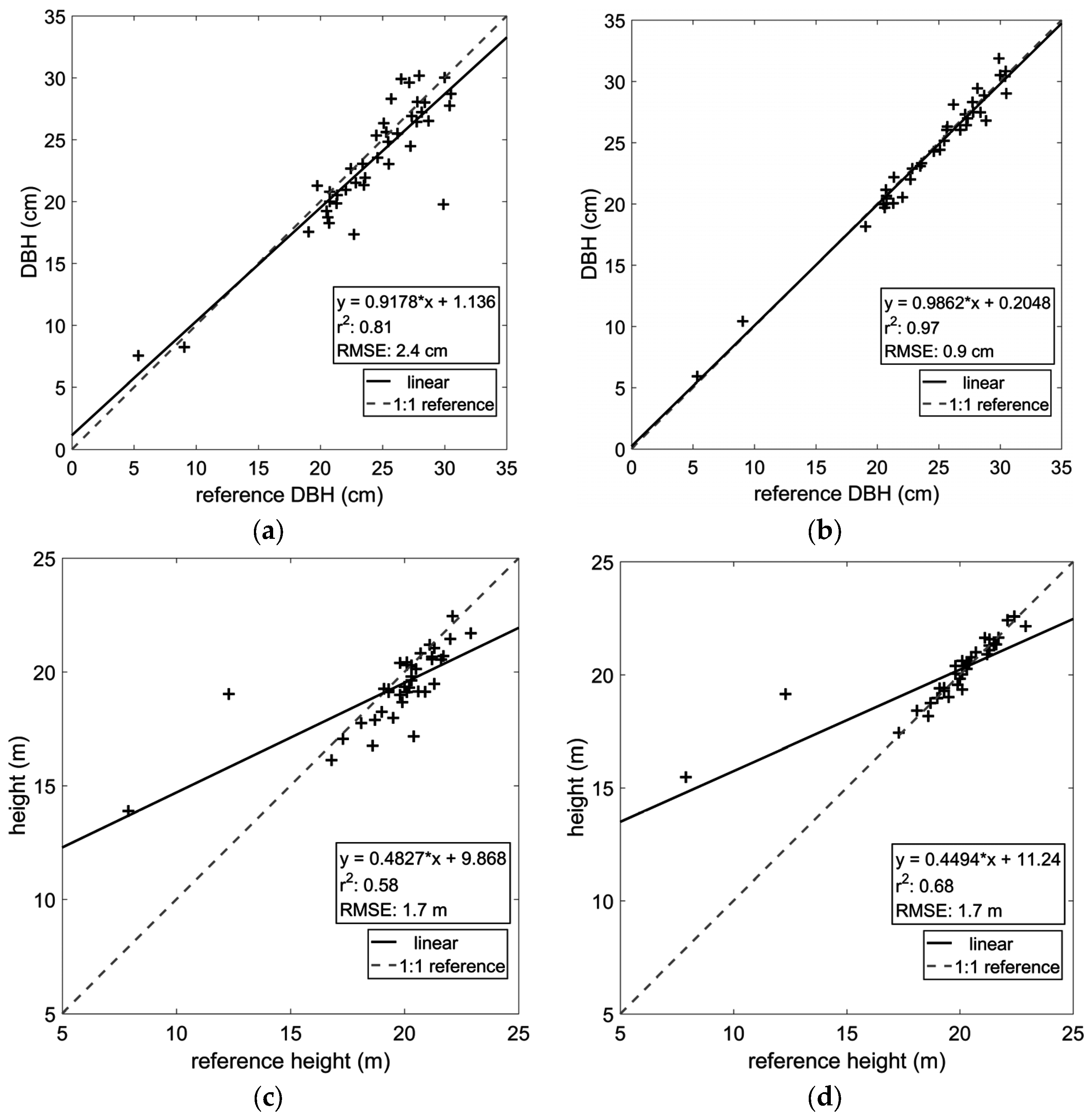
Figure 9.
Scatter plot between range and DBH error: (a) from single scan (SS); (b) from MS. Here, error is defined as the absolute difference between the measured ground truth and the extracted.
Figure 9.
Scatter plot between range and DBH error: (a) from single scan (SS); (b) from MS. Here, error is defined as the absolute difference between the measured ground truth and the extracted.

Figure 10.
Scatter plot between relative tree height and diameter error: (a) from SS; (b) from MS. Here, error is defined as the absolute difference between the measured diameters and the extracted.
Figure 10.
Scatter plot between relative tree height and diameter error: (a) from SS; (b) from MS. Here, error is defined as the absolute difference between the measured diameters and the extracted.


Table 1.
Parameter and settings for automated stem attribute analysis from terrestrial laser scanning (TLS) data.
| 1. DTM extraction | ||
| DTM resolution | 0.2 (m) | |
| * | Local elevation tolerance in a moving window | 0.5 (m) |
| Minimum initial ground points in a moving window | 10 | |
| * | DTM upper threshold factor | 5 |
| 2. Stem detection | ||
| Horizontal resolution for voxelization | 0.1 (m) | |
| Vertical resolution for voxelization | 0.5 (m) | |
| * | Cylindrical filter width s (roughly close to DBH) | 0.2 (m) |
| Cylindrical filter height b | 1 (m) | |
| Maximally-allowed cylindrical filter leaning angle | 20° | |
| * | Cylindrical filter value (larger value creates more peaks) | 1 |
| Filtered peak detection strength (larger value detects weaker peaks) | 0.5 | |
| 3. Branch and stem segmentation | ||
| * | Region growing step | 0.02 (m) |
| Point gap tolerance | 0.01 (m) | |
| * | Maximum branch width increase ratio | 0.8 |
| Maximum branch direction change | 60° | |
| 4. Stem curve extraction | ||
| Stem node interval | 0.2 (m) | |
| * | Stem radius tolerance | 1.3 |
* Controlling parameters.
| RMSE | r2 | |
| DBH (SS) | 2.4 cm | 0.81 |
| DBH (MS) | 0.9 cm | 0.97 |
| Height (SS) | 1.7 m | 0.58 |
| Height (MS) | 1.7 m | 0.68 |
| Average RMSEs | Average r2 s | |
| Diameter (SS) | 3.2 cm | 0.58 |
| Diameter (MS) | 2.4 cm | 0.76 |
| Process | SS | MS |
|---|---|---|
| Reading point cloud | 1 | 4 |
| (sppm) * | (2.5) | (2.2) |
| Extracting and removing DTM | 1 | 4 |
| (sppm) | (2.5) | (2.2) |
| Extracting stem location | 0.2 | 1 |
| (sppm) | (0.5) | (0.5) |
| Isolating stem space | 1 | 4 |
| (sppm) | (2.5) | (2.2) |
| Extracting stem form | 24 | 135 |
| (sppm) | (61.1) | (72.9) |
| Overall | 27 | 148 |
| (sppm) | (68.7) | (80.0) |
* Seconds per million points (sppm).
© 2016 by the authors; licensee MDPI, Basel, Switzerland. This article is an open access article distributed under the terms and conditions of the Creative Commons Attribution (CC-BY) license (http://creativecommons.org/licenses/by/4.0/).
Share and Cite
MDPI and ACS Style
Xi, Z.; Hopkinson, C.; Chasmer, L. Automating Plot-Level Stem Analysis from Terrestrial Laser Scanning. Forests 2016, 7, 252. https://doi.org/10.3390/f7110252
AMA Style
Xi Z, Hopkinson C, Chasmer L. Automating Plot-Level Stem Analysis from Terrestrial Laser Scanning. Forests. 2016; 7(11):252. https://doi.org/10.3390/f7110252
Chicago/Turabian StyleXi, Zhouxin, Christopher Hopkinson, and Laura Chasmer. 2016. "Automating Plot-Level Stem Analysis from Terrestrial Laser Scanning" Forests 7, no. 11: 252. https://doi.org/10.3390/f7110252
Note that from the first issue of 2016, this journal uses article numbers instead of page numbers. See further details here.