Article

Enhancing Forest Growth and Yield Predictions with Airborne Laser Scanning Data: Increasing Spatial Detail and Optimizing Yield Curve Selection through Template Matching

1
Faculty of Forestry, University of British Columbia, 2424 Main Mall, Vancouver, BC V6T 1Z4, Canada
2
Canadian Forest Service (Pacific Forestry Centre), Natural Resources Canada, 506 West Burnside Road, Victoria, BC V8Z 1M5, Canada
*
Author to whom correspondence should be addressed.
Forests 2016, 7(11), 255; https://doi.org/10.3390/f7110255
Submission received: 13 July 2016 / Revised: 15 October 2016 / Accepted: 22 October 2016 / Published: 28 October 2016
(This article belongs to the Special Issue LiDAR Remote Sensing of Forest Resources)

Abstract

:
Accurate information on both the current stock and future growth and yield of forest resources is critical for sustainable forest management. We demonstrate a novel approach to utilizing airborne laser scanning (ALS)-derived forest stand attributes to determine future growth and yield of six attributes at a sub-stand (25 m grid cell) level of detail: dominant height (HMAX), Lorey’s height (HL), quadratic mean diameter (QMD), basal area (BA), whole stem volume (V), and trees per hectare (TPH). The approach is designed to find the most appropriate matching yield curve and project the attributes to the age of 80 years. Comparisons to conventional plot-level projections resulted in relative mean differences of 13.4% (HMAX), −27.1% (HL), 18.8% (QMD), 12.0% (BA), 18.6% (V), and −17.5% (TPH). The respective relative root mean squared difference values were: 31.1%, 38.4%, 19.8%, 19.8%, 21.8%, and 38.4%. Differences were driven mostly by stand-level age and site index. The uncertainty of cell-level yield curve assignment was used to refine stand-level summaries. The novel contribution of this study is in the application of growth and yield models at the cell level, combined with the use of ALS-derived attributes to optimize yield curve selection via template matching.

1. Introduction

Sustainable management of forest ecosystems requires accurate information on forest composition and structure. This data, collected during forest inventories, provides information on forest stand attributes and their extent, driving many management decisions, such as date of harvest and silvicultural practices. Since forest ecosystems are dynamic and continuously changing, it is necessary to project certain forest stand attributes forward in time to support forest planning and forest management [1]. As a result, knowledge of the spatial distribution of the timber and related dimensions, both for current management, and into the future for advanced yield prediction, is crucial for long-term planning as well as financial and environmental sustainability [2].
Foresters use growth models to project stand attributes to a desired future age [1]. Being an abstraction of the natural dynamics of a forest stand, growth models are typically a system of equations that can predict forest growth and yield under a variety of conditions [3,4]. Growth models can generally be divided into three groups, according to the level of abstraction: (1) whole stand models; (2) size-class models; and (3) single-tree models. Whole-stand models are the simplest, however, they are insufficient when information on size class or individual trees is required [3]. Single-tree models are the most-detailed, with each individual tree as the basic unit of modelling; however, the approach requires a tree list that specifies the DBH (diameter at breast height) and height of every tree in the stand as input data. Size-class models are a compromise between whole-stand models and single-tree models and provide some information on both stand structure and individual tree attributes (e.g., histogram of DBH) [3]. All three types of models are based on multiple stand characteristics, with site quality (i.e., site index or SI) often being among the most important characteristics for modelling growth. As an indirect measure of site quality, SI evaluates tree height relative to tree age and is considered the most practical and consistent indicator of site quality [1]. In addition to the three aforementioned statistical growth models, process-based models, which focus on modelling the physiological processes of growth, including photosynthesis and respiration, can also be used, but have historically been less operationally applied than statistical methods [5].
Airborne laser scanning (ALS) data can be used to estimate forest stand attributes that are relevant for both operational and strategic forestry needs [6]. ALS point clouds provide metrics that are useful for predicting attributes of forest stands and provide the capacity to generate both bare ground and canopy height models. The point clouds can be used to estimate tree or stand height, and through statistical modelling, can provide information on a comprehensive set of predicted stand characteristics that include basal area, DBH, volume, and biomass. The capacity of a given laser beam to penetrate through gaps in the forest canopy generates an ALS point cloud distributed across most of the vertical profile of a forest stand. Metrics that summarize this point cloud distribution (e.g., descriptive statistics, percentiles, proportions) are related to forest attributes and are used as independent variables in the modelling [7,8].
ALS-based predictions of forestry-related attributes can be performed following two approaches: individual tree detection (ITD) [9], or area-based approach (ABA) [8]. ITD is based on treetops or tree crowns that are initially located on either raw ALS point cloud on canopy height models [10,11]. This method is therefore prone to errors resulting from under- or over-segmentation of tree crowns [12]. Alternatively, the ABA is based on metrics that summarize the distribution of the point cloud within a single pixel (typically 20–30 m on a side), which then become independent variables in the modeling process. Due to reliability and ease of implementation, ABA is widely used operationally over a range of forest environments [13,14]. While ABA approaches have become common practice in many jurisdictions, the explicit link to future growth and yield estimates is often complicated. ABA approaches offer cell-based representations of the standing forest stock (such as volume and height) with limited information on species composition, while conventional inventories provide polygon based species information with estimates of volume based on field data or growth models.
Although different approaches may be used to estimate forest growth with remote sensing tools, the most common approach utilizes the relationship between growth and tree dimensions [15]. These approaches can be divided into two categories. First, growth can be assessed based on two measurements (separated by an interval of time) of the same tree or stand, with measurement differences directly indicating the growth. Second, remote sensing can provide input data to parametrize existing growth models. Most studies using the first approach focus on estimating height differences based on multiple ALS acquisitions, as height is the attribute that can be determined directly and with highest accuracy [16,17,18]. To our knowledge, only a few examples exist that demonstrate how ALS data can be linked directly to a whole-stand or single-tree growth and yield models. Härkönen et al. [19] demonstrated how a simplified process-based model can be simulated with input data derived from ALS point clouds, at the individual tree level. Similarly, Taguchi et al. [20] used ALS-derived input data with the 3PG model (Physiological Principles to Predict Growth; [21]) to predict future stem biomass with yield table values. Falkowski et al. [22] used ALS-predicted individual tree attributes as input values for the Forest Vegetation Simulator (FVS), a growth model widely applied in United States [23]. FVS operates at the individual tree level and requires tree species and DBH for parametrization. Additional inputs, like general site condition description, site index, and stand density may improve the growth estimates. Falkowski et al. [22] found that, in general, the growth projections from the inventory and ALS-predicted stand attributes followed similar trends and concluded that ALS data has great potential for detailed individual tree-level inventories.
While growth and yield models offer the capacity to predict future forest growth, the choice of the most appropriate yield curve for a given stand is based on multiple input variables that describe a forest stand and that are acquired during forest inventory. Limitations associated with the measurement of these stand attributes include visual assessment (and thus some subjectivity) of some of the relevant parameters (such as canopy closure), as well as inherent error in the inventory measurements themselves (such as in height and therefore site index). These limitations can lead to incorrect yield curve assignment which in turn has ramifications for the subsequent forest management decisions [3,4]. ALS provides a unique opportunity to improve growth and yield modelling by offering improved estimates of the relevant parameters that leads to more precise selection of appropriate yield curve. In addition, by integrating growth and yield curves with ALS predictions, we can ensure that for the same forest stand, the predicted ALS attributes (such as stand height, mean DBH, and canopy cover) are all internally consistent with what is expected for a given species and site combination. The role of a growth model can therefore be extended—to not only provide information on projected yield, but also to ensure that all the estimated attributes correspond to the same yield curve, and as a result represent more realistic combinations of stand size approximations.
In this paper, we develop a method to enhance forest growth and yield modelling with area-based inputs predicted from ALS data. We demonstrate how multiple ALS-predicted estimates of stand attributes can be used to inform the selection of the most optimal growth and yield curve through a process of template matching. Concurrently, we show how sub-stand variability of those estimates can be transferred to growth and yield projections, resulting in stand growth information at the 25 m raster cell-level. To do so, we utilize ALS-predicted raster layers that provide cell-level information on current stand height, quadratic mean diameter, and volume. First, we generate a database of yield curve templates from a growth and yield model using the full range of required input parameters derived from inventory data. Second, we assign a set of unique yield curves to each cell by matching ALS-predicted stand attributes with yield curve templates, with additional input from inventory data. We report uncertainty in yield curve assignment through the template matching and we compare the projected cell-level attributes with stand-level projections calculated using conventional forest inventory data. Finally, we identify those factors that contribute to the observed discrepancies between stand- and cell-level projections of forest attributes and discuss implications for forest management and planning. By demonstrating the potential of this approach we aim to offer a novel method that allows incorporation of ALS data into growth and yield estimation, thereby extending the benefits of ALS point clouds beyond estimating standing stock inventory attributes and embed it more into the entire growth and yield inventory cycle.

2. Materials and Methods
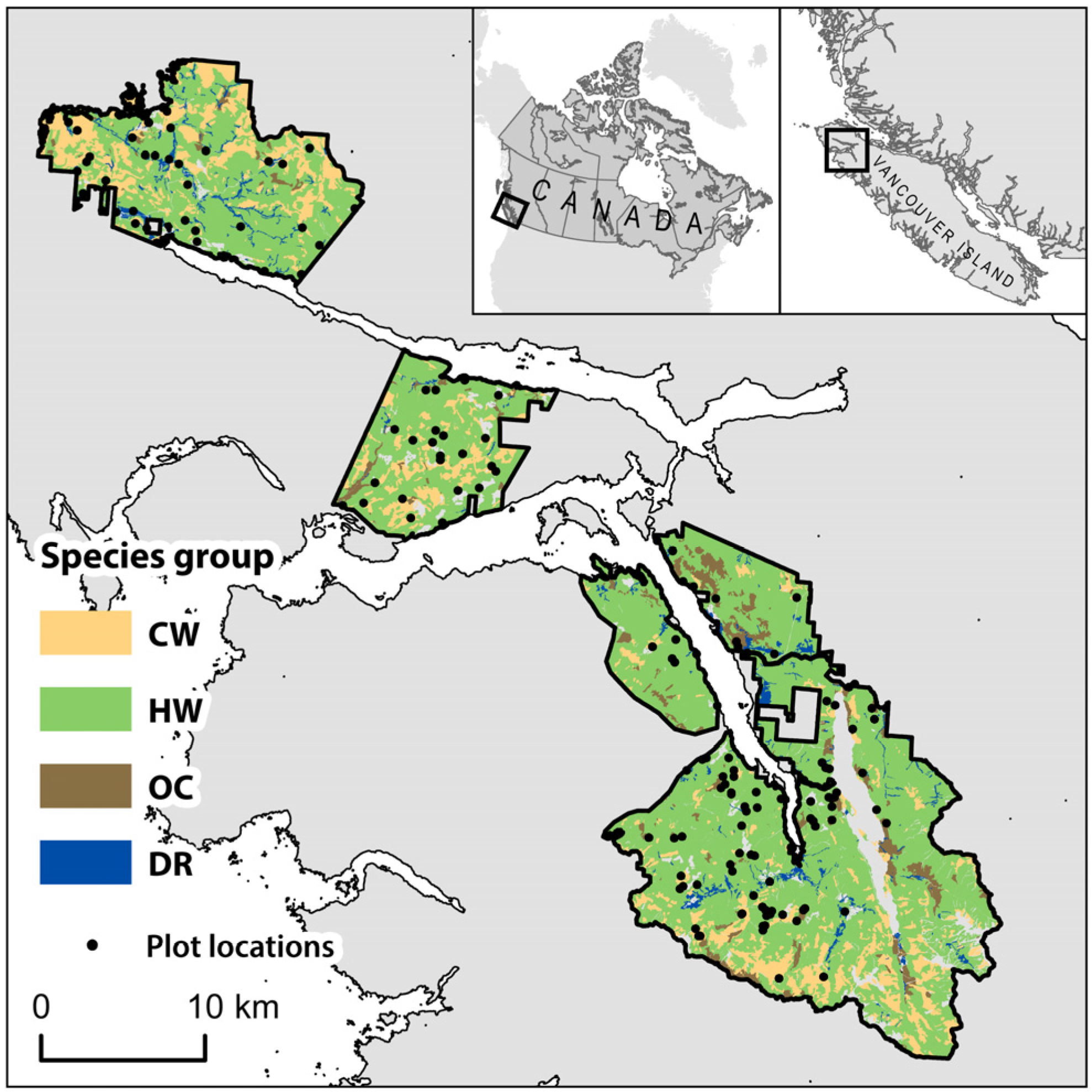
2.1. Study Area

The study area was located on northern Vancouver Island, British Columbia, Canada and is approximately 52,000 ha in size (Figure 1). Located within the Coastal Western Hemlock (CWH) biogeoclimatic zone, the study area is characterized by high annual precipitation (2228 mm), mild winters, and cool summers [24]. Elevation within study area ranges from sea level to 1200 m, with an average slope of 23.6°. This area contains highly productive, temperate rainforest stands dominated by western hemlock (Tsuga heterophylla). Other common tree species in the study area included western red cedar (Thuja plicata), Douglas-fir (Pseudotsuga menziesii), red alder (Alnus rubra), amabilis fir (Abies amabilis), yellow cedar (Chamaecyparis nootkatensis), mountain hemlock (Tsuga mertensiana), and Sitka spruce (Picea sitchensis). The average age of stands was 146 years (σ = 127 years). The high site productivity results in the mean annual increment (MAI) of volume often exceeding 20 m3·ha−1·year−1 [25,26].

2.2. Forest Inventory Data

A strategic-level forest inventory, compiled according to standard provincial forest inventory procedures (i.e., air photo interpreters delineated homogenous forest stands and interpreted attributes such as age, height, and species composition) was used as reference data [27]. Attributes, such as DBH, volume, species, age, and site index were modeled and validated with field plot measurements as part of the inventory process [28]. Stand attributes including mean DBH, Lorey’s height, and volume, were projected forward to the year 2012 to provide single, consistent temporal reference for all stands [29]. The average length of these projections was six years, with the majority of inventory data collected in 2012.
The forest inventory in the study area contained 5586 stands and represented a total area of 59,150 ha with eight unique dominant tree species (Table 1). Stands were aggregated into four groups according to the dominant species: HW—stands dominated by western or mountain hemlock, CW—stands dominated by western redcedar or yellow cedar; OC—stands dominated by other coniferous species; and DR—stands dominated by deciduous species, which consisted of red alder only. The inventory data was used to compare with the results of the ALS-predicted growth and yield at the stand level.

2.3. Ground Plot Data

Field data collected on 133 forest inventory plots were used to evaluate the growth and yield projections predicted from the ALS data. Plots were circular with a radius of 14 m (area = 615.75 m2) and plot centres were recorded with sub-metre accuracy using a Trimble GeoXH GPS receiver with an external Tornado antenna and differential correction. The plot measurements consisted of DBH, height, and species. A sample of two trees were cored to determine the age for each plot. Only live standing trees with a DBH ≥12 cm were measured. Individual tree measurements were aggregated to generate plot-level estimates of Lorey’s mean height (HL), quadratic mean diameter (QMD), basal area (BA), and volume (V). A summary of plot characteristics, by species group, is provided in Table 2.

2.4. ALS Point Clouds and Metrics

Optech ALTM3100EA scanning system was used to acquire ALS point clouds in 2012. The average first return point density was 11.6 points/m2 (details related to ALS data acquisition can be found in Tompalski et al. [30]). Returns classified as “ground” were used to create a Digital Terrain Model (DTM). The DTM raster layer with a pixel size of 1 m was then used to normalize point cloud heights to heights above ground level. ALS-derived metrics were calculated for each forest stand polygon using FUSION (version 3.42). These metrics, used as independent variables in regression modelling, consisted of measures of central tendency (mean, median, mode), spread (standard deviation, interquartile distance, coefficient of variation), percentiles and proportions of normalized point heights.

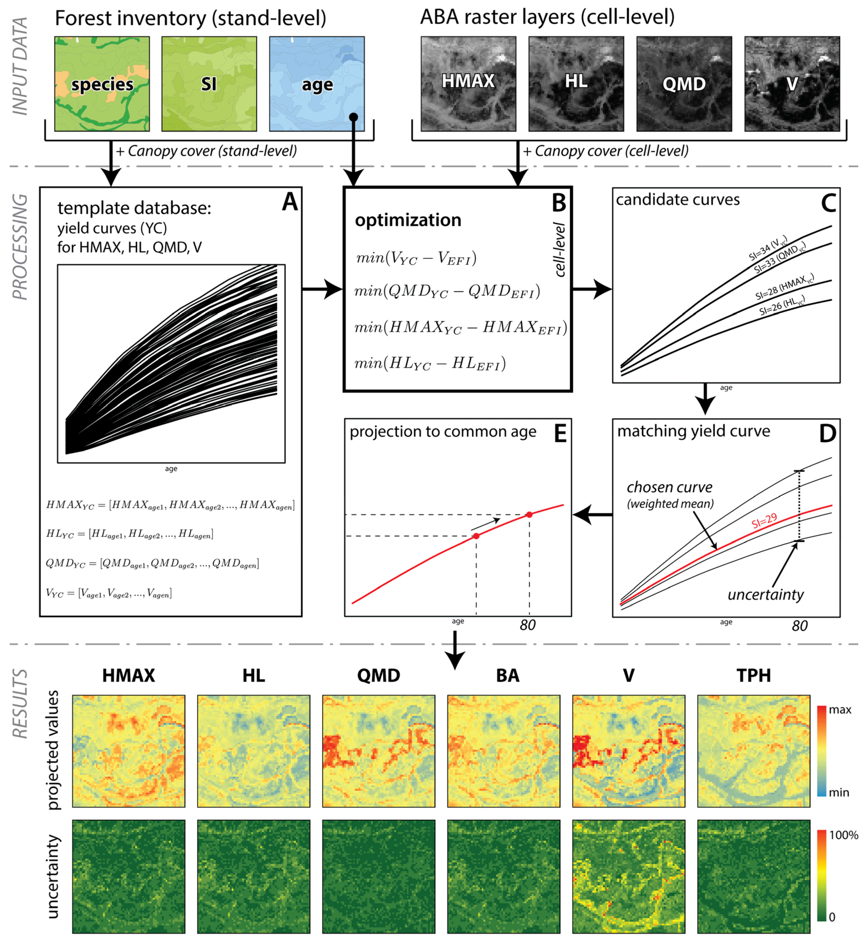
2.5. Enhanced Forest Inventory Data

Forest inventories that incorporate information predicted from ALS data are referred to as enhanced forest inventories (EFI) [6]. EFI typically consist of wall-to-wall predictions of stand height (maximum height, Lorey’s height), canopy cover, basal area, quadratic mean diameter, and volume (e.g., whole stem volume), estimated using an area-based approach (ABA; [8]). These predictions are typically generated as raster layers with a cell size between 20 and 30 m. Assigning predicted stand attributes to raster cells instead of polygon representations of stands provides additional details of internal stand variability for all predicted attributes and in general much finer grain than traditional forest inventories. The ability of ALS data to describe the dimensions and structure of a forest stand results in high accuracy of such predictions, with typical RMSE (Root Mean Square Error) for volume of about 20%–30% [31,32,33].
For our study area ABA-predicted layers were generated using multiple linear regression with chosen ALS-derived metrics as independent variables. Plot-level data was used as reference information on the modelled attributes (dominant height—HMAX, Lorey’s height—HL, quadratic mean diameter—QMD, and whole stem volume—V, all at 12.5+ utilization level). Separate models were created for each of the dominant species for QMD and V, resulting in four separate models for these attributes. Mean difference (MD) and root mean square difference (RMSD) values for the models are presented in Table 3. Wall-to-wall raster layers generated with these models were used as input data in our study. The timber utilization level defines the minimum dimensions of timber that is actually cut and removed from a forest stand [34]. A utilization level of 12.5+ defines the minimum dimension of timber as 12.5 cm inside bark diameter, 30 cm stump height, and 10 cm inside bark top diameter.

2.6. Growth and Yield Model

Two forest growth models are currently used by the Ministry of Forests, Lands and Natural Resource Operations in British Columbia: Table Interpolation for Stand Yields (TIPSY) and Variable Density Yield Projection (VDYP). TIPSY is designed for single-species, even-aged, managed stands [25], while VDYP can predict growth and yield in stands with more complex structure, and is suitable for unmanaged stands [26]. VDYP and TIPSY are both stand-level growth and yield models.
In this study, we used VDYP (version 7) due to the unmanaged status, age, and complexity of the forest stands in the study area. VDYP predicts yields by incrementing stand age and height, as well as density attributes including basal area and quadratic mean diameter [35]. The minimal set of input parameters includes species, dominant height, age, Lorey’s height, and basal area. These input parameters can be augmented by information on site index, biogeoclimatic zone, and canopy cover. A stand description created using these input parameters is projected forward or backward depending on current stand age and desired projection age [26].
The results of the predictions include stand attributes for the desired age sequence. VDYP predicts HL, HMAX, QMD, basal area (BA), trees per hectare (TPH) and five different volume types: whole stem volume; close utilization; close utilization net decay; close utilization net decay and waste; and close utilization net decay, waste and breakage. Outputs are generated at chosen utilization limit (4.0 cm+, 7.5 cm+, 12.5 cm+, 17.5 cm+, and 22.5 cm+), indicating minimum inside bark diameter.

2.7. Generation of Yield Curve Templates

In order to assign an appropriate yield curve to each ABA-cell, we used VDYP to populate a yield curve template database that contains all possible yield curves for all possible stand conditions within the study area (Figure 2A). We used the existing inventory data to define the range of required input parameters, for each dominant species including stand age (from 1 to maximum stand age, by 1 year increments, Table 1) and site index (from minimal to maximal SI value, by 1 m). Additionally, we varied canopy cover (in 10% classes) calculated from the ALS data as a proportion of first returns above 2 m to all returns. Predictions were generated for a utilization level of 12.5 cm+, similar to the utilization level used during the ABA modelling. The reference age (a target age used in all growth and yield analysis) was set to 80 years, the most common rotation age in the study area. The final database therefore consisted of yield curve (YC) templates that included the four input variables: HMAX, HL, QMD, and V, predicted for different percentage of canopy cover, site index, and age.
Once the database of yield curve templates was populated, a yield curve was assigned for each 25 m cell corresponding to raster layers predicted with ABA. First, candidate curves were selected from the yield curve template database based on age and species from the inventory and a minimal difference between ABA-predicted attribute and value of a yield curve at a given stand age (Figure 2B). This allowed us to choose four candidate curves, which differed in site index value (Figure 2C).
The final yield curve (YCC) was chosen by calculating a weighted mean of the four candidate site index values, with the percent of explained variance in the ABA model used as a weight (Figure 2D). We therefore assigned more weight to stand attributes that were modeled with higher accuracy:
Y C C = R H M A X 2 H M A X Y C + R H L 2 H L Y C + R Q M D 2 Q M D Y C + R V 2 V Y C R H M A X 2 + R H L 2 + R Q M D 2 + R V 2
where:
  • R x 2 —coefficient of determination of ABA-predicted attribute x; x = (HMAX, HL, QMD, V)
  • x Y C —candidate yield curve chosen for attribute x
The final results consisted of all VDYP predictions at 80 years (Figure 2E), together with the corresponding uncertainties. From the available outputs of VDYP growth and yield model, we chose six attributes of interest: HL, HMAX, QMD, BA, V, and TPH.
Additional detail on forest stands was provided once a yield template was assigned to each cell. The yield curve was used to estimate current annual increment (CAI) and mean annual increment (MAI) curves for V, per cell. CAI is the yearly growth rate, while MAI informs on the growth over the whole period from origin to a specific age. Together these curves inform on growth pattern of the stand within each cell and are of particular interest to forest managers, as the intersection of CAI and MAI curves informs on theoretical optimal harvest age that maximizes timber productivity [1]. The optimal harvest age was estimated for each cell and summarized with mean, median, mode, and standard deviation.

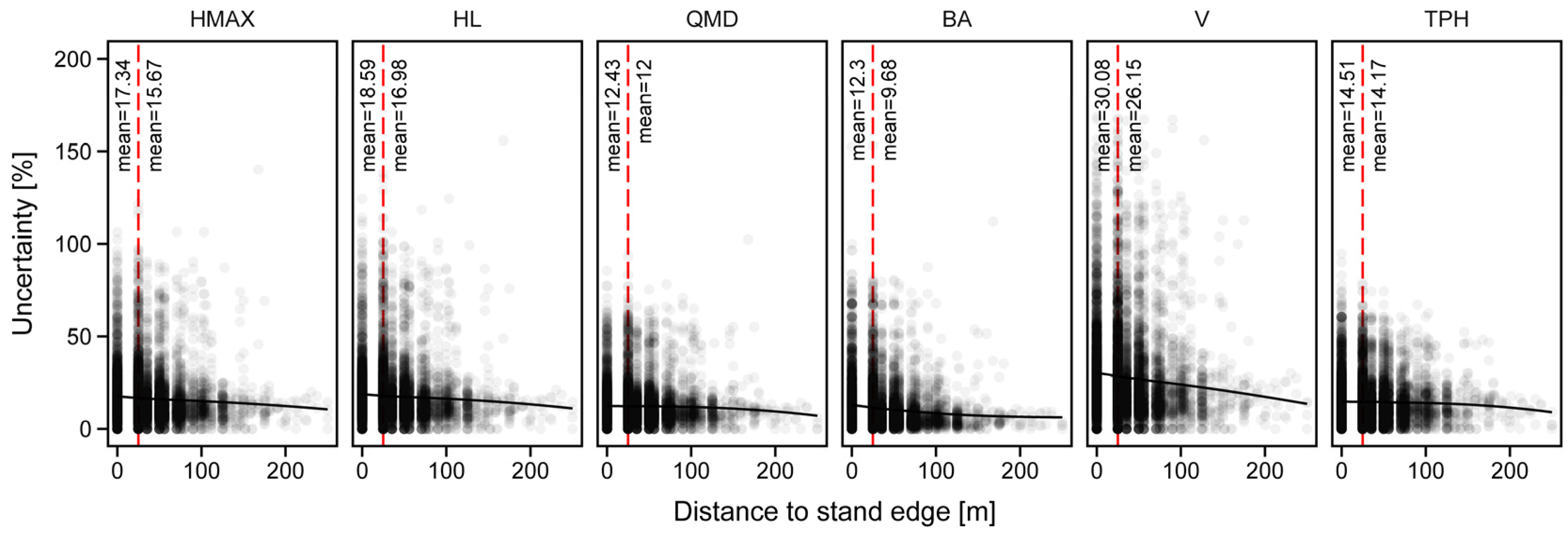
2.8. Evaluation of Uncertainty in Yield Curve Assignment

The uncertainty of the curve assignments (∆x) for each of the six VDYP-predicted variables x was described as the absolute value of a relative difference between a value of stand attribute on a chosen yield curve (xC) and a value on a curve with the largest difference to the chosen one (xmax):
Δ x = | x m a x x C x C | 100
The uncertainty was therefore a measure of the agreement between ABA-predicted stand attributes (HMAX, HL, QMD, V) and the growth model stand templates. We evaluated the relationship between the magnitude of uncertainty and the location of a cell relative to the stand boundary. To assure that the uncertainty values are independent, a random sample representing 1% of all cells was chosen for the analysis. The differences between uncertainty values on stand edges and stand cores were assessed using a t-test (α = 0.05). Lastly, we also analyzed the relationship of the relative differences between the attributes and inventory data, with multiple stand-level attributes that included age, site index, species, projection type: forward/backward, stand area, and number of years projected. The Random Forest variable importance metric [36] was used to uncover the underlying relationship between projections and selected factors and evaluate its magnitude.

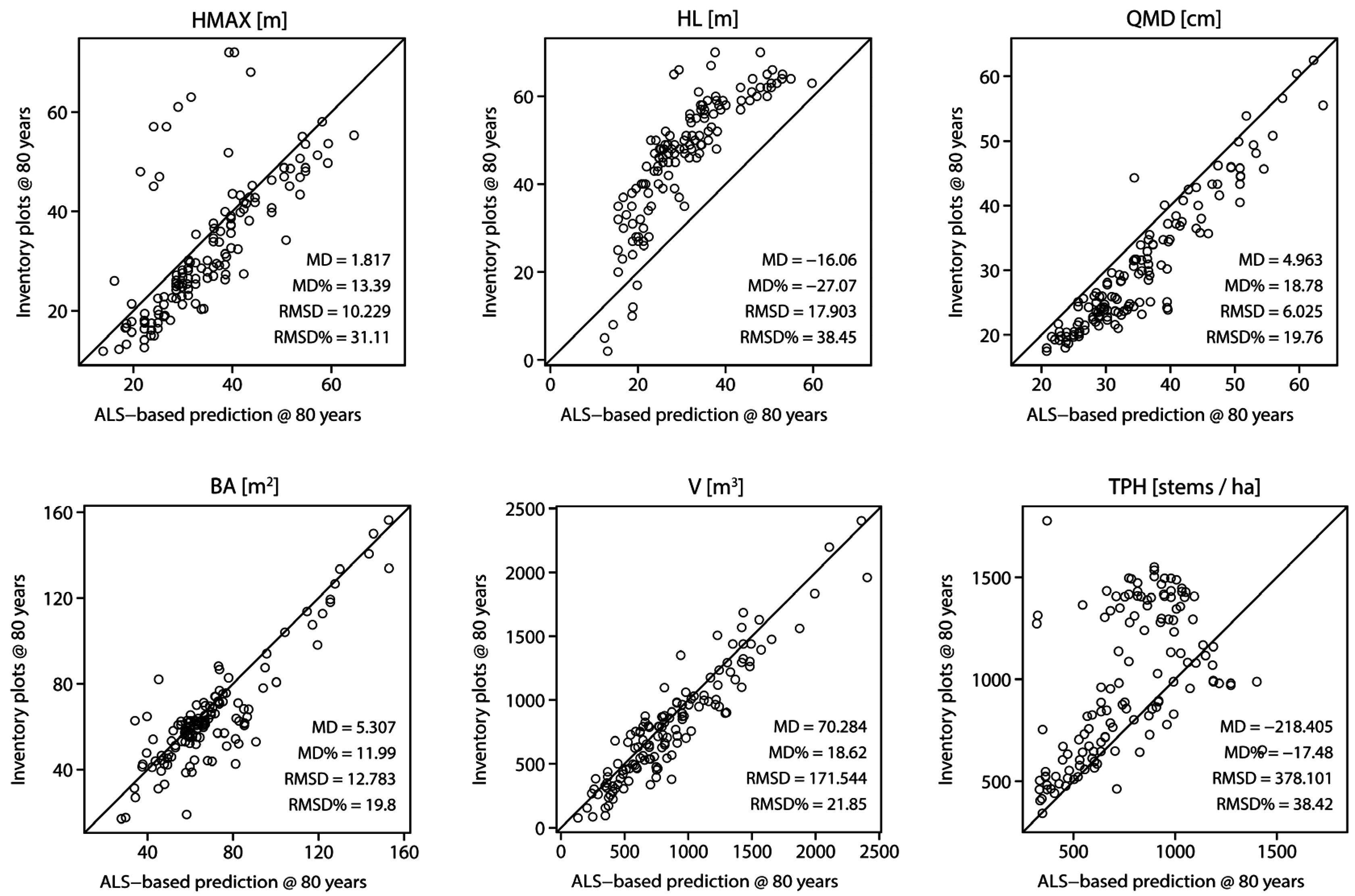
2.9. Evaluation of Attribute Projections

Our model-based projections of HMAX, HL, QMD, BA, V, and TPH generated from the ALS-predicted rasters were evaluated using stand-level forest inventory and ground plot data. The inventory and ground plot data were each input to the growth and yield model, resulting in separate reference projections at 80 years for all six attributes at both the stand and plot level. We used these reference projections to evaluate the VDYP projections from the ALS-predicted rasters. To allow for comparisons at the stand level, within-stand, ALS-based cell-level projections were averaged to the stand level. To reduce stand edge effects, stand polygon area was reduced by applying an inner buffer of 25 m; cells within this buffer distance were excluded from the calculation of stand-level averages. To allow for comparisons at the plot level, ALS-based cell-level projections for cells within a 3 by 3 cell window surrounding the ground plot centroid were averaged. We compared model predictions using the mean difference (MD, absolute and relative) and RMSD (root mean square difference, absolute and relative) and used a paired t-test to evaluate the null hypothesis that the means of the two compared variables are equal (at α = 0.05). MD and RMSD were calculated as follows:
M D = 1 N i = 1 N ( y ^ i y i )
M D % = M D y ¯ 100
R M S D = 1 N i = 1 N ( y ^ i y i ) 2
R M S D % = R M S D y ¯ 100
where: N is the number of stands or plots, yi is the inventory based (plot or stand) projected value, ŷi is the ALS-based predicted value for stand i, and ȳ is the mean of the inventory variable.

3. Results

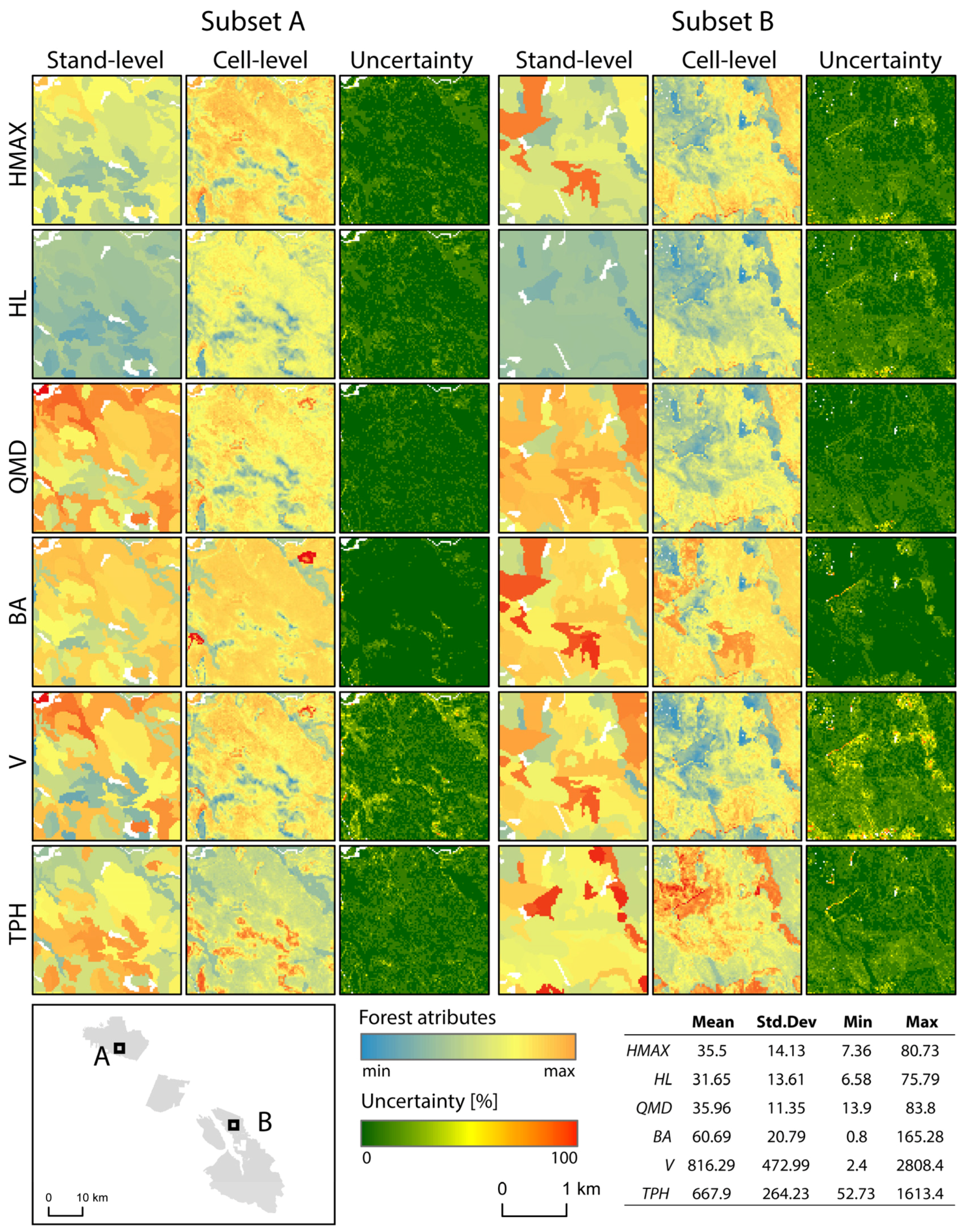
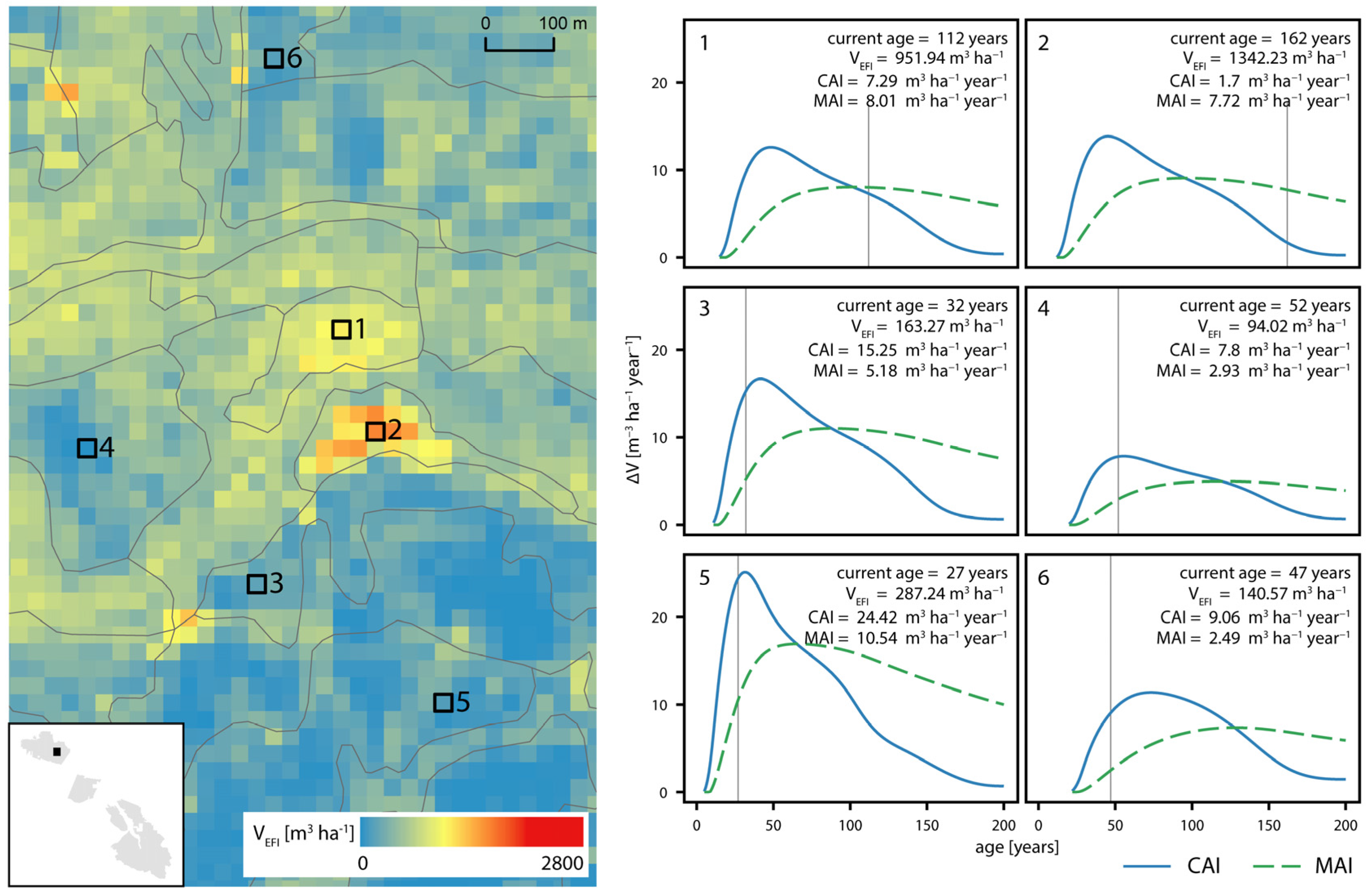
3.1. Attribute Projections

Predictions for the six chosen stand attributes (HMAX, HL, QMD, BA, V, and TPH) were generated at the cell level and averaged to provide stand- and plot-level values for comparison. Cell-level predictions were estimated using ABA layers predicted from ALS data, with additional information on stand age and species composition from the conventional stand-level inventory data. The conventional inventory data was used to generate a yield curve template database that consisted of 1,811,230 individual yield curves. A spatial subset of the results, which consisted of raster layers of projected attributes at both the stand- and cell-level, as well as the calculated uncertainty values, are presented in Figure 3.
Our approach resulted in a yield curve assignment to each of the 25 m raster cells. These yield curves were used to predict attributes at the age of 80 years and generate growth curves. Figure 4 demonstrates CAI and MAI growth curves assigned to a chosen subset of cells. These cells are located within stands that differ in age, site index, and dominant species and therefore reveal different patterns in volume increments. These patterns inform on slow (e.g., cell 4), medium (e.g., cell 1), or fast (e.g., cell 5) growth rates. It can be observed how the optimal rotation age, defined with the maximum of the MAI curve, differs among exemplar cells, being lower for cells with large growth rates (e.g., cell 5) and higher for cells that show slower growth (e.g., cell 4). For the entire study area, the optimal harvest age, based on MAI curve maximum, had a unimodal distribution with a mean value of 83.3 years, a standard deviation of 24.5 years, a median equal to 81 years, and a mode equal to 81 years.

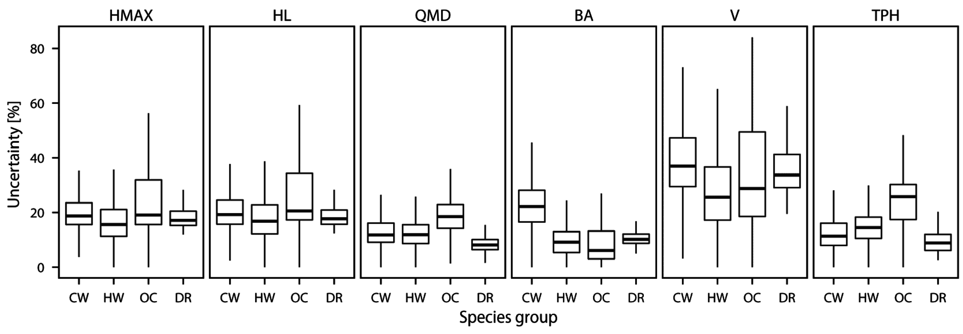
3.2. Evaluation of Uncertainty in Yield Curve Template Assignment

The uncertainty of yield curve template assignment, which we define as the largest relative difference between the chosen yield curve template and all possible candidate curves for that attribute, was summarized for every variable (Figure 5). The largest uncertainty values were observed for V, which had the highest median value and the largest range. Uncertainties for other variables were lower and more similar to each other, with the lowest median and range observed for QMD. Among species groups, the largest median uncertainties were observed for the “other conifer” group, with one exception for volume, where “CW” group had the largest value of 38.0%.
Uncertainty values had a relationship with distance to stand edge (Figure 6). For all stand attributes a similar trend was observed of uncertainty values decreasing with the distance from stand edge. When grouped into two categories, edge (cells with distance to edge less or equal 25 m) and core, the mean uncertainty was always significantly larger for edge cells (t-test, α = 0.05). As a result, a negative buffer of 25 m was applied to the stand polygons during stand-level attribute projections.

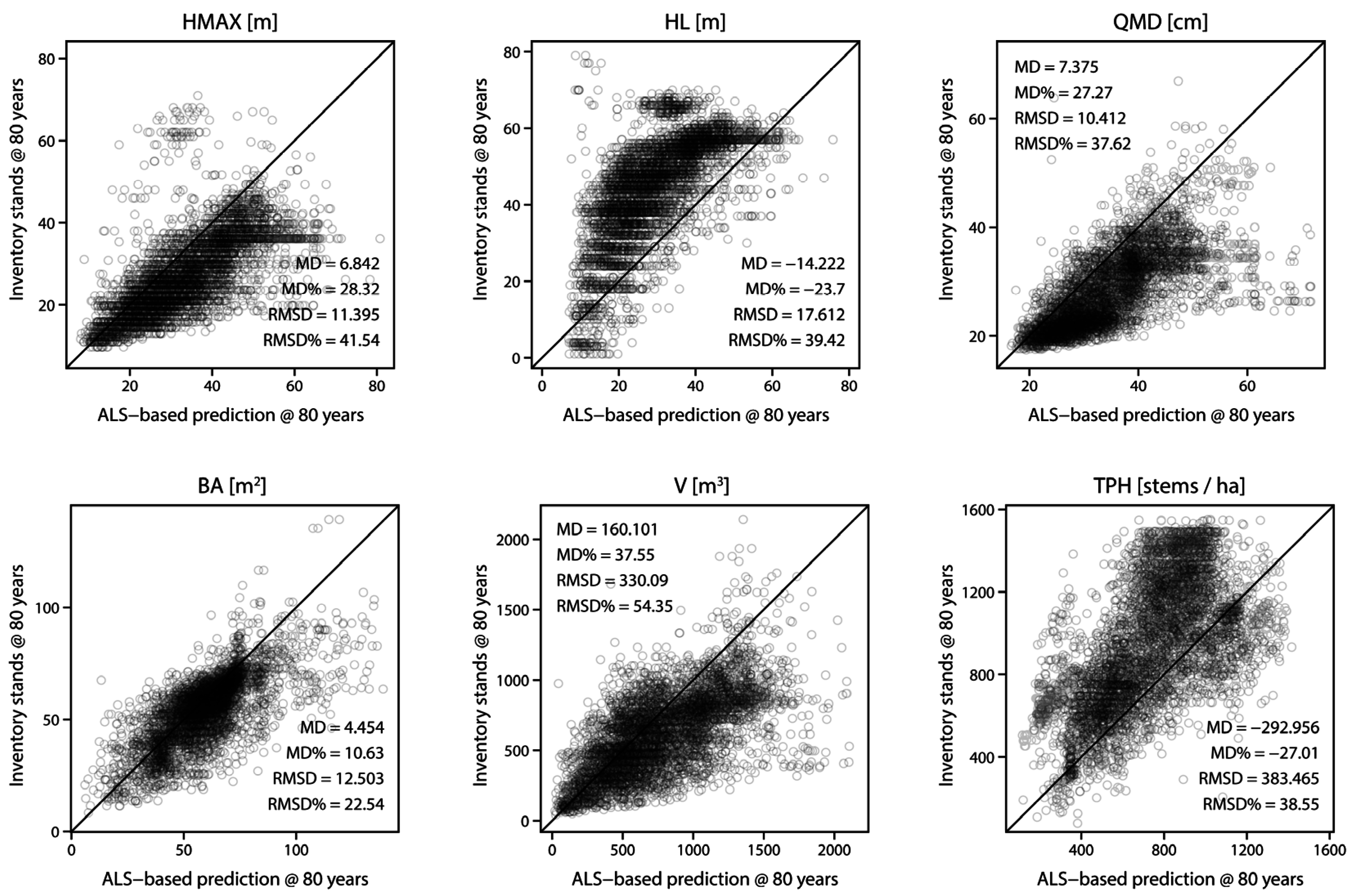
3.3. Evaluation of Attribute Projections

The results of the comparison of the stand-level and cell-level attribute projections are presented in Table 4, Figure 7 and Figure 8. The relative MD (Figure 7) was positive for all but two stand attributes, with the largest values observed for V. Similarly, the largest values of relative RMSD were also observed for V. Among species groups, relative RMSD values were higher for CW and DR. The highest relative MD of 81.0% was observed for DR species group in V. All p-values were less than 0.01.
Comparison performed at the plot level (Figure 8) with field measured data projected to 80 years was very similar to comparisons at the stand-level. Similarly, the MD for the majority of the attributes was positive. Small RMSD values were observed for HMAX, QMD, BA, and V, with relative RMSD for V = 21.85%. These four stand attributes showed strongest agreement with field measurements at the projected age of 80 years. Similarly, as for stand-level comparison, HL was underestimated, with relative MD of −27.07%. Underestimation was also observed for TPH, especially for denser stands with number of trees per ha over 800.
Variable importance derived with Random Forest showed that the percent of explained variance was above 60% for almost all attributes, with largest values of 79.4 and 77.7 for HL and TPH, respectively (Figure 9). The importance of the analyzed factors varied across forest attributes, with SI frequently found as the most important, notably greater than the importance of the other factors. Stand area, projection type (forward or backward), years projected, and stand age were among the least important factors, although importance of stand age and years projected still exceeded 20% for all attributes. The importance of the dominant species was moderate when compared with other factors, with values between 20% for HL and almost 100% for HMAX.

4. Discussion

In this research, ALS-based cell-level predictions of multiple forest stand attributes, stand-level inventory data, and growth models were combined to predict stand growth and yield at a 25 m level of abstraction. The proposed methodology described herein allows managers to assign growth and yield curves to each 25 m cell by matching predicted stand attributes with a database of yield curve templates. Since ALS can be used to predict a suite of attributes with ABA, including volume, DBH, and height, the selection of the yield curve can take advantage of all these potential sources of information. This additional benefit over the standard approach of growth and yield modelling ensures that the predicted attributes correspond to each other, but also to predicted uncertainty in yield curve assignment based on the discrepancies between site index values for each of the candidate curves.
Our approach was based on two steps. First, we generated a comprehensive database of yield curve templates utilizing existing photo-based stand-level forest inventory information to determine upper and lower limits for each of the required input parameters. Each of the yield curve templates represented a forest stand with a constant site index and species composition (dominant species only), and a changing set of stand attributes with age increments. Second, we used ABA-predicted attributes to assign a yield curve to each ABA cell. Since four ABA-predicted stand attributes were used (HMAX, HL, QMD, and V) as inputs, a final yield curve was chosen based on four candidate yield curves. The largest relative difference between the chosen curve and the other candidate curves was reported as uncertainty.
Uncertainty of yield curve assignment results from disagreement between the set of ABA-predicted stand attributes (HL, HMAX, QMD, and V), and is reflected by different site index values of the candidate yield curves. Therefore, during yield curve matching, an updated site index value is assigned to an ABA cell using weighted mean. Knowing that ABA predictions are not error-free, we assigned more weight to predictions for which there was greater confidence (higher percentage of variance explained). Hence, in general, the uncertainties in yield curve assignment were related to the accuracies of the ABA predictions, resulting in lower uncertainty for attributes like HL or HMAX, and higher uncertainty for V. The process of averaging the site index and the final assignment of the yield curve resulted in modification of the stand attributes (both decrease and increase) to match the corresponding yield curve. From the available stand attributes predicted with the yield model we demonstrate six attributes (HMAX, HL, QMD, BA, V, TPH) that together provide a comprehensive set of information on forest characteristics within each cell. This included also information on stand density—a parameter that was not included as model input, and was therefore exclusively a result of growth model predictions. This shows how existing ABA products can be used to enrich available information on forest stands.
Uncertainty resulted from the discrepancies between ABA predictions. Since the input data we used represented two different levels of detail, with ABA predictions of HMAX, HL, QMD, and V at the cell-level, and estimates of age and species composition at the stand level, uncertainty analysis allowed us to avoid unreasonable age and stand attribute pairs that existed especially on stand edges. Reducing the area of the stand polygons was therefore important and allowed us to exclude the cells with higher uncertainty from the computation of stand-level summaries. Additionally, for extreme cases such situations resulted in no yield curve assignment, as the yield curve templates were limited by minimum and maximum site index values recorded in the study area as a whole. An example of such situation is a forest gap for which the ABA metrics show low height, DBH, and volume values, and do not correspond to the age and SI values of the stand. The summation of cell-level predictions to the stand level is often desired by forest managers (due to planning or regulatory requirements), and these stand-level predictions can therefore be made more reliable by incorporating the information generated from the uncertainty analysis.
Our method of yield curve assignment via our optimized template matching approach, as demonstrated herein, enabled us to characterize growth of the stand within each 25 m cell. CAI and MAI curves informed on current and future increments in stand attribute values, and these curves can provide an additional set of information for forest managers. Most commonly, the maximum of the MAI curve, which is also the point of intersection between CAI and MAI curves, indicates the most efficient volume production over time. It is also considered the ideal rotation age, however, tree dimensions, pathogens, and other factors are not taken into account. By calculating the optimal harvest age for the whole study area, we found that the most frequent value (mode) was 81 years, which corresponds to the rotation age currently used in the area. However, with the presented method it is also possible to define stands for which the rotation age should be increased or could be lowered, resulting in potentially more efficient timber production.
Information on stand growth assigned to each cell provided an opportunity to simulate future within-stand volume distribution depending on a chosen harvesting routine. In the demonstrated examples the projected attributes were a result of two scenarios that assumed no harvesting activities in the first case, or strict stand removal at 80 years in the second. Although both scenarios represent extreme and not realistic management decisions, they provided boundaries for possible volume distributions across the chosen projection years and demonstrated how volume distribution changes after certain activities. This allows observation of how the management decisions made at cell-level influence forest stands at the larger extent.
The comparison of stand-level, inventory-based growth and yield modeling and cell-level predictions averaged to stand level, demonstrated that by incorporating ABA-predicted inventory growth and yield estimates were larger than using standard plot data for almost all modelled forest stand attributes. This observation was confirmed by comparing projections at the plot level, with field collected data used as reference. At the stand level, the largest differences were observed for whole stem volume (V), with a relative MD of 41.7% and relative RMSD of 58.1%. At the plot level, a strong agreement was observed between BA and V, with relative RMSD of 19.8% and 21.85%, respectively. At both comparison levels, negative differences (cell-level predictions lower than the reference values) were only observed for HL and TPH. The positive MD for whole stem volume is similar to that of a recent study that examined how ALS data could be used to augment site index estimation [30]. In that study, it was found that ALS-predicted dominant stand heights were significantly different when compared to existing photo-based inventory data (+3.5 m), and that the volumes calculated with the ALS-based and original site index values were larger by an average of 51.5%. Moreover, as discussed by Tompalski et al. [30], the largest differences in volume estimates were found for stands dominated by western red cedar. In the Tompalski et al. [30] study, it is postulated that the reason for the differences in volume estimates for western red cedar is that only 0.6% of western red cedar stands are pure, single species stands. Most of the stands are composed of two or more species, with western hemlock being the most common co-occurring species. At a given age, western red cedar is typically shorter than western hemlock [37,38].
Our analysis confirmed that site index was the prevalent driver of the differences between inventory-based growth and yield modelling and cell-level predictions. This result was expected, as during the choice of the optimal yield curve, site index value was modified depending on the HMAX, HL, QMD, and V. Stand age and number of years projected were among the least important factors. The differences were also not significantly influenced by the type of the projection (forward or backward). Although stand age was shown to not be the most important factor influencing the difference between inventory- and ALS-based projections, we acknowledge that information on stand age is crucial for accurate modelling of growth and yield. Among all of the input variables used during growth projections, age is the most difficult to estimate with remote sensing tools [39,40]. However, with the increasing length of the available record of satellite imagery, particularly Landsat, forest stand age becomes possible to map at cell level [39,40]. For younger stands, such information can be then incorporated into the presented methodology.
Enhanced growth and yield modelling with ABA-predicted, cell-level attributes of forest stands used as input information, allows users to maintain the additional, cell-level detail obtained using ALS and ABA approaches when projecting the attributes to the desired age. This additional level of detail allows the examination of differences in growth patterns at sub-stand level. Furthermore, finding the optimal yield curve for each cell, based on multiple ABA-predicted attributes, provides a unique opportunity to ensure that the discrepancy between the input attributes is minimized. The adjustment of the attributes during yield curve matching reduces the disagreement between them and the uncertainty shows where such discrepancy exists, thereby allowing for improved stand level summaries.

5. Conclusions

In this study we used an innovative template matching approach, combined with the enriched spatial detail and accuracy enabled by ALS-predicted forest inventory attributes, to optimize the selection of growth and yield curves for subsequent cell-level growth and yield modelling. Unique to our approach is the utilization of a broad suite of ALS-predicted attributes, including maximum height, Lorey’s height, quadratic mean diameter, and whole stem volume, to assign the most suitable and internally consistent yield curve template at the cell- and stand-level. To facilitate template selection, we first generated a comprehensive template database that consisted of yield curves for all possible combinations of site index, canopy cover, dominant species, and age. Additionally, we accounted for any mismatch during yield curve assignment and used it to increase reliability of stand-level summaries.
The growth and yield model we used in our study are typically applied at the stand level, hence our application of these models to individual raster cells is novel and takes advantage of ABA outputs. The results of our study indicate that overall, cell-level modelling resulted in larger estimates for stand attributes compared to conventional yield projections on both the stand- and plot-level. Differences between our results and those of conventional stand- and plot-level yield projects were primarily caused by our reliance on stand-level age and site index information predicted from the conventional forest inventory data for the area.
ALS data and the ABA allow for detailed cell-level enhancements to refine growth and yield modelling. The particular benefits of the approach we present herein include improved within-stand spatial detail, optimization of yield curve selection, and the capacity to incorporate spatial uncertainty into stand-level estimates of projected attributes of interest. Improvements to growth and yield modelling can provide many benefits for sustainable forest management and planning. Forest regulators can benefit from improved long-term planning of allowable annual harvest levels, while forest managers can benefit from improved selection of stands for harvest or silvicultural intervention. Likewise, carbon budget models are often based upon use of growth and yield models, with the predictions of volume used to estimate biomass and in-turn, model carbon. Across this varied range of applications, additional utility is offered by the ability to refine model selection, track the relative role of contributing variables, and to undertake scenario development and simulations. ALS data is well established and reliable for measurements of forest structure and forest inventory attributes. In this research, we have offered a means to benefit from this detailed and spatially explicit characterization of forest structure to improve and quantify projections of future forest characteristics using established and understood forest inventory protocols and practices. The template matching approach provides a novel method to refine the selection of appropriate growth and yield curves, while also providing users with a means to understand error and alternate growth trajectories based upon given forest and site characteristics.

Acknowledgments

This research was supported by the Canadian Wood Fibre Centre (CWFC) of the Canadian Forest Service, Natural Resources Canada. Mike Davis of Western Forest Products Inc. is thanked for sharing the data used in this research. Support was also provided by a Natural Sciences and Engineering Research Council of Canada (NSERC) grant to Nicholas Coops.

Author Contributions

The authors contributed equally to the overall research design, approach and analysis. The lead author wrote early drafts of the manuscript with contributions from the other authors through the editorial process.

Conflicts of Interest

The authors declare no conflict of interest.

References

  1. Avery, T.E.; Burkhart, H. Forest Measurements; McGraw-Hill: New York, NY, USA, 2002. [Google Scholar]
  2. Wulder, M.A.; Bater, C.W.; Coops, N.C.; Hilker, T.; White, J.C. The role of LiDAR in sustainable forest management. For. Chron. 2008, 84, 807–826. [Google Scholar] [CrossRef]
  3. Pretzsch, H. Forest Dynamics, Growth and Yield: From Measurement to Model; Springer: Berlin, Germany, 2009; pp. 1–39. [Google Scholar]
  4. Peng, C. Growth and yield models for uneven-aged stands: Past, present and future. For. Ecol. Manag. 2000, 132, 259–279. [Google Scholar] [CrossRef]
  5. Mäkelä, A.; Landsberg, J.O.E.; Ek, A.R.; Burk, T.E.; Ter-Mikaelian, M.; Ågren, G.I.; Oliver, C.D.; Puttonen, P. Process-based models for forest ecosystem management: Current state of the art and challenges for practical implementation. Tree Physiol. 2000, 20, 289–298. [Google Scholar] [CrossRef] [PubMed]
  6. White, J.C.; Wulder, M.A.; Varhola, A.; Vastaranta, M.; Coops, N.C.; Cook, B.D.; Pitt, D.; Woods, M. A best practices guide for generating forest inventory attributes from airborne laser scanning data using an area-based approach. For. Chron. 2013, 89, 722–723. [Google Scholar] [CrossRef]
  7. Bouvier, M.; Durrieu, S.; Fournier, R.A.; Renaud, J.-P. Generalizing predictive models of forest inventory attributes using an area-based approach with airborne LiDAR data. Remote Sens. Environ. 2015, 156, 322–334. [Google Scholar] [CrossRef]
  8. Næsset, E. Predicting forest stand characteristics with airborne scanning laser using a practical two-stage procedure and field data. Remote Sens. Environ. 2002, 80, 88–99. [Google Scholar] [CrossRef]
  9. Hyyppä, J.; Inkinen, M. Detecting and estimating attributes for single trees using laser scanner. Photogramm. J. Finl. 1999, 16, 27–42. [Google Scholar]
  10. Reitberger, J.; Schnörr, C.; Krzystek, P.; Stilla, U. 3D segmentation of single trees exploiting full waveform LiDAR data. ISPRS J. Photogramm. Remote Sens. 2009, 64, 561–574. [Google Scholar] [CrossRef]
  11. Jakubowski, M.; Li, W.; Guo, Q.; Kelly, M. Delineating Individual Trees from LiDAR Data: A Comparison of Vector- and Raster-based Segmentation Approaches. Remote Sens. 2013, 5, 4163–4186. [Google Scholar] [CrossRef]
  12. Maltamo, M.; Eerikainen, K.; Pitkanen, J.; Hyyppa, J.; Vehmas, M. Estimation of timber volume and stem density based on scanning laser altimetry and expected tree size distribution functions. Remote Sens. Environ. 2004, 90, 319–330. [Google Scholar] [CrossRef]
  13. Brosofske, K.D.; Froese, R.E.; Falkowski, M.J.; Banskota, A. A review of methods for mapping and prediction of inventory attributes for operational forest management. For. Sci. 2014, 60, 733–756. [Google Scholar] [CrossRef]
  14. Wulder, M.A.; Coops, N.C.; Hudak, A.T.; Morsdorf, F.; Nelson, R.; Newnham, G.; Vastaranta, M. Status and prospects for LiDAR remote sensing of forested ecosystems. Can. J. Remote Sens. 2013, 39, S1–S5. [Google Scholar] [CrossRef]
  15. Coops, N.C. Characterizing Forest Growth and Productivity Using Remotely Sensed Data. Curr. For. Rep. 2015, 1, 195–205. [Google Scholar] [CrossRef]
  16. Yu, X.; Hyyppä, J.; Kaartinen, H.; Maltamo, M. Automatic detection of harvested trees and determination of forest growth using airborne laser scanning. Remote Sens. Environ. 2004, 90, 451–462. [Google Scholar] [CrossRef]
  17. Hopkinson, C.; Chasmer, L.; Hall, R.J. The uncertainty in conifer plantation growth prediction from multi-temporal LiDAR datasets. Remote Sens. Environ. 2008, 112, 1168–1180. [Google Scholar] [CrossRef]
  18. Næsset, E.; Gobakken, T. Estimating forest growth using canopy metrics derived from airborne laser scanner data. Remote Sens. Environ. 2005, 96, 453–465. [Google Scholar] [CrossRef]
  19. Härkönen, S.; Tokola, T.; Packalén, P.; Korhonen, L.; Mäkelä, A. Predicting forest growth based on airborne light detection and ranging data, climate data, and a simplified process-based model. Can. J. For. Res. 2013, 43, 364–375. [Google Scholar] [CrossRef]
  20. Taguchi, H.; Endo, T.; Yasuoka, Y. Biomass estimation by coupling LiDAR data with forest growth model in conifer plantation. In Proceedings of the 28th Asian Association of Remote Sensing Conference, Kuala Lampur, Malaysia, 12–16 November 2007; pp. 4–6.
  21. Landsberg, J.J.; Waring, R.H. A generalised model of forest productivity using simplified concepts of radiation-use efficiency, carbon balance and partitioning. For. Ecol. Manag. 1997, 95, 209–228. [Google Scholar] [CrossRef]
  22. Falkowski, M.J.; Hudak, A.T.; Crookston, N.L.; Gessler, P.E.; Uebler, E.H.; Smith, A.M.S. Landscape-scale parametrization of a tree-level forest growth model: A k-nearest neighbor imputation approach incorporating LiDAR data. Can. J. For. Res. 2010, 40, 184–199. [Google Scholar] [CrossRef]
  23. Dixon, G. Essential FVS: A User’s Guide to the Forest Vegetation Simulator; Internal Report; USDA: Fort Collins, CO, USA, 2003.
  24. Meidinger, D.V.; Pojar, J. Ecosystems of British Columbia; British Columbia Ministry of Forests: Victoria, BC, Canada, 1991.
  25. Ministry of Forest Lands and Natural Resource Operations. Growth and Yield Modelling. Available online: https://www.for.gov.bc.ca/hts/growth/tipsy/tipsy_description.html (accessed on 10 June 2015).
  26. British Columbia Ministry of Forests. Variable Density Yield Projection; Forest Analysis and Inventory Branch: Victoria, BC, Canada, 2009.
  27. Ministry of Forest Lands and Natural Resource Operations. Vegetation Resources Inventory, Version 3.0; Photo Interpretation Procedures: Victoria, BC, Canada, 2014.
  28. Leckie, D.G.; Gillis, M.D. Forest inventory in Canada with emphasis on map production. For. Chron. 1995, 71, 74–88. [Google Scholar] [CrossRef]
  29. Sandvoss, M.; Mcclymont, B.; Farnden, N.C. A User’s Guide to the Vegetation Resources Inventory; Tolko Industries, Ltd.: Williams Lake, BC, Canada, 2005. [Google Scholar]
  30. Tompalski, P.; Coops, N.C.; White, J.C.; Wulder, M.A. Augmenting site index estimation with airborne laser scanning data. For. Sci. 2015, 61, 861–873. [Google Scholar] [CrossRef]
  31. Maltamo, M.; Packalén, P.; Suvanto, A.; Korhonen, K.T.; Mehtätalo, L.; Hyvönen, P. Combining ALS and NFI training data for forest management planning: A case study in Kuortane, Western Finland. Eur. J. For. Res. 2009, 128, 305–317. [Google Scholar] [CrossRef]
  32. Kankare, V.; Räty, M.; Yu, X.; Holopainen, M.; Vastaranta, M.; Kantola, T.; Hyyppä, J.; Hyyppä, H.; Alho, P.; Viitala, R. Single tree biomass modelling using airborne laser scanning. ISPRS J. Photogramm. Remote Sens. 2013, 85, 66–73. [Google Scholar] [CrossRef]
  33. Woods, M.; Pitt, D.; Penner, M.; Lim, K.; Nesbitt, D.; Etheridge, D.; Treitz, P. Operational implementation of a LiDAR inventory in Boreal Ontario. For. Chron. 2011, 87, 512–528. [Google Scholar] [CrossRef]
  34. Ministry of Forests, Lands & Natural Resource Operations. Glossary of Forestry Terms in British Columbia. Available online: https://www.for.gov.bc.ca/hfd/library/documents/glossary/ (accessed on 20 October 2015).
  35. Ministry of Forest Lands and Natural Resource Operations. Growth Relationships and Model Components. Available online: https://www.for.gov.bc.ca/hts/vri/biometric/bio_growth.html (accessed on 10 June 2015).
  36. Breiman, L. Random forest. Mach. Learn. 2001, 45, 5–32. [Google Scholar] [CrossRef]
  37. Smith, J.H.G.; Ker, J.W.; Czizmazia, J. Economics of Reforestation of Douglas-fir, Western Hemlock and Western Red Cedar in the Vancouver Forest District; University of British Columbia: Vancouver, BC, Canada, 1961. [Google Scholar]
  38. Minore, D. Western Redcedar: A Literature Review; USDA: Portland, OR, USA, 1983.
  39. Tompalski, P.; Coops, N.C.; White, J.C.; Wulder, M.A.; Pickell, P.D. Estimating Forest Site Productivity Using Airborne Laser Scanning Data and Landsat Time Series. Can. J. Remote Sens. 2015, 41, 232–245. [Google Scholar] [CrossRef]
  40. Pickell, P.D.; Hermosilla, T.; Coops, N.C.; Masek, J.G.; Franks, S.; Huang, C. Monitoring anthropogenic disturbance trends in an industrialized boreal forest with Landsat time series. Remote Sens. Lett. 2014, 5, 783–792. [Google Scholar] [CrossRef]
Figure 1. Study area location with species groups distribution and inventory plot locations. Species group abbreviations explained in Table 1.
Forests 07 00255 g001
Figure 2. An outline of the processing steps. SI—site index; HMAX—dominant height, HL—Lorey’s height, QMD—quadratic mean diameter, BA—basal area, V—whole stem volume, TPH—trees per hectare. Boxes A–E are explained in detail in the text.
Forests 07 00255 g002
Figure 3. Two subsets of stand attribute predictions at stand- and cell-level, and their respective uncertainties. Descriptive statistics calculated for the cell-level predictions are presented in the bottom-right corner of the figure.
Forests 07 00255 g003
Figure 4. Current annual increment (CAI) and mean annual increment (MAI) curves for six exemplar cells located in different forest stands. The left panel represents a subset of the study area with the current volume estimates derived with EFI modeling (VEFI), stand borders (grey lines), and the location of the chosen cells. The right panel contains CAI and MAI curves for these cells. Grey vertical lines depict the current age assigned to each cell. Text boxes contain information on cell age, volume, and current growth (CAI and MAI).
Forests 07 00255 g004
Figure 5. Uncertainty values of yield curve assignment for stand inventory variables.
Forests 07 00255 g005
Figure 6. Relationship between distance to stand edge and uncertainty among predicted variables. Dashed red line indicates the division between border and core cells (distance = 25 m). Black solid line indicates loess trend line.
Forests 07 00255 g006
Figure 7. Comparison of six chosen forest stand attributes projected to 80 years at stand-level. Observed values are derived by projecting stand attributes, whereas predicted values are derived with the proposed method and averaged to stand level.
Forests 07 00255 g007
Figure 8. Comparison of six chosen forest stand attributes projected to 80 years at plot-level. Observed values are derived by projecting field measurements, whereas predicted values are derived with the proposed method.
Forests 07 00255 g008
Figure 9. Importance of stand age (AGE), site index (SI), dominant species (SP), forward or backward projection method (F/B), stand area (AREA), and number of years projected (YP) calculated with random forest for relative differences between cell- and stand-level prediction of inventory attributes.
Forests 07 00255 g009
Table 1. Forest stand characteristics in the study area.
Species GroupCommon NameScientific NameSpecies CodeTotal AreaMean Area (ha)Number of StandsStand Age (Years)Stand Height (m)Site Index (m)
ha%#%meanσmeanσmeanσ
HWwestern hemlockTsuga heterophylla Sarg.Hw42,673.272.16.6648967.9132.3118.422.216.422.26.6
mountain hemlockTsuga mertensiana (Bong.) Carr.Hm1742.92.98.32112.2242.947.523.25.76.82.5
group subtotal44,416.175.16.6670070.1135.8118.422.216.221.77.1
CWwestern redcedarThuja plicata Donn ex D. DonCw7379.212.54.9149315.6215.4149.621.215.916.94.8
yellow-cedarChamaecyparis nootkatensis (D. Don) SpachYc2521.44.36.73763.9251.8127.616.59.411.75.1
group subtotal9900.616.75.3186919.6222.7146.120.214.915.95.3
OCDouglas-firPseudotsuga menziesii (Mirb.) FrancoFd740.01.37.41001.0116.2101.024.015.727.45.9
amabilis firAbies amabilis Douglas ex J. ForbesBa1199.02.05.32252.4106.4101.517.817.021.06.0
Sitka sprucePicea sitchensis (Bong.) Trautv. & C. A. Mey.Ss940.51.66.91371.462.376.116.415.631.56.7
group subtotal2880.74.96.24644.995.396.718.716.525.47.8
DRred alderAlnus rubra Bong.Dr1953.33.33.75265.553.117.221.27.024.75.8
total for all stands59,150.7100.06.29559100.0146.2127.721.615.620.97.3
Table 2. Inventory plots characteristics for the four species groups.
Species GroupnHL (m)QMD (cm)V (m3)
MeanσMeanσMeanσ
CW1830.66.147.711.21107.9466.6
HW10034.210.442.115.61032.1598.6
OC731.69.135.212.6933.8439.0
DR824.17.627.68.1462.3323.3
Overall13333.010.041.615.11002.9575.5
Species group abbreviations explained in Table 1. Hl—Lorey’s mean height; QMD—quadratic mean diameter; V—volume.
Table 3. Enhanced forest inventory (EFI) modelling results.
VariableSpeciesR2 b i a s ^ *RMSERMSE%
HMAX (m)All0.950.002.536.65
HL (m)All0.940.012.407.93
QMD (cm)HW0.71−0.828.9520.49
CW0.37−0.677.9117.68
OC0.29−0.0713.3429.79
DR0.79−0.602.618.56
V (m3)HW0.6810.12334.3634.13
CW0.48−33.47303.7133.54
OC0.54−34.56276.1031.89
DR0.7611.07128.2826.30
Summary information gathered from an internal documentation obtained from Western Forest Products Inc. HMAX—dominant height; HL—Lorey’s mean height; QMD—quadratic mean diameter; V—Gross Biological Volume. All attributes calculated at 12.5 cm utilization level. * b i a s ^ = 1 N i = 1 N ( y ^ i y i ) , where N is the number of reference plots, yi is the observed value, and ŷi is the predicted value.
Table 4. Results of the comparison between inventory-based projections and cell-level projections based on airborne laser scanning (ALS)-derived attribute predictions.
Forest Stand AttributeSpecies GrouprMDMD%RMSDRMSD%
HMAX (m)CW0.724.4823.5510.5353.17
HW0.808.2331.6011.0739.45
OC−0.02−7.27−8.2519.1741.84
DR0.226.5627.619.6134.42
all0.766.8428.3211.3941.54
HL (m)CW0.62−14.77−22.6820.2257.12
HW0.81−12.90−21.9115.4734.19
OC0.74−15.34−30.5417.7635.72
DR0.14−32.66−50.0633.0750.67
all0.74−14.22−23.7017.6139.42
QMD (cm)CW0.665.5721.2311.4743.26
HW0.838.1530.1410.4538.36
OC0.674.8516.619.1527.03
DR0.123.9313.125.7717.36
all0.787.3727.2710.4137.62
BA (m2·ha−1)CW0.7913.1928.9921.1838.11
HW0.692.345.488.8515.78
OC0.295.4517.5920.5930.11
DR0.195.3919.529.1227.76
all0.734.4510.6312.5022.54
V (m3·ha−1)CW0.67107.3935.90402.1283.64
HW0.69170.0735.26311.4749.09
OC0.73145.9437.65355.0240.68
DR0.24207.4581.01301.5778.77
all0.67160.1037.55330.0954.35
TPH (stems·ha−1)CW0.38−73.64−5.98263.6627.23
HW0.81−371.62−34.36420.8340.08
OC0.44−72.38−5.74282.5435.70
DR0.09−38.60−5.88101.1326.11
all0.69−292.96−27.01383.4638.55
r—Pearson correlation coefficient.

