The Biodiversity Benefits and Opportunity Costs of Plantation Forest Management: A Modelling Case Study of Pinus radiata in New Zealand

Abstract

This study modelled the potential biodiversity benefits and the opportunity costs of a patch-clear-cutting strategy over a clear-cutting strategy for Pinus radiata in New Zealand. Patch-clear cutting is a special case of clear cutting involving the removal of all the trees from strips or patches within a stand, leaving the remainder uncut or clear cutting a series of strips or patches. A forest-level optimisation model was extended to include uncertainty in timber growth, plant diversity, and cutting costs. Using a species-area relationship and economies of cutting scale, the net present value and optimal rotation age under alternative management strategies were calculated. Results suggested that the optimal rotation ages were similar (24 and 25 years) for the two cutting strategies. Patch-clear cutting provided higher biodiversity benefits (i.e., 59 vs. 11 understorey plant species) with an opportunity cost of 27 NZD (18 USD) per extra plant species or 1250 NZD (820 USD) ha⁻¹. However, the true benefits of patch-clear cutting would be even greater if other benefits of stand retention are included. Our research can potentially inform local decision making and inform international systems of payment for environmental services, such as the REDD+ (Reducing Emissions from Deforestation and Forest Degradation) program, to conserve biodiversity in developing countries with plantation forests.

1. Introduction

Forests are among the most important providers of ecosystem services [1]. Forests are home to more than half of the known terrestrial plant and animal species [2], and deforestation is the major cause of biodiversity loss [3,4]. Since the global annual rate of natural forest loss is 0.3% [5] and appears difficult to reverse, plantation forests may sometimes be a “lesser evil” compared to agricultural land as a means to protect indigenous vegetation remnants [6]. Plantation forests are defined as forests of predominantly introduced species established through planting and/or seeding, and forests of native species established through planting and/or seeding and managed intensively [5]. Although only accounting for 7% of total forest cover world-wide, plantation forests provide approximately 50% of total wood production [5]. Moreover, there is abundant evidence that plantation forests can provide habitat for a wide range of native forest plants, animals, and fungi. For example, exotic tree plantations can provide important conservation services to protected areas [7]. There is a range of 48 to 135 indigenous and adventive vascular plant species per stand of Pinus radiata plantations in New Zealand [3].

Several common cutting methods have been applied in plantation forests around the world, such as clear cutting, patch-clear cutting, and selection cutting [8]. The dominant cutting strategy for commercial forests in many countries from temperate, boreal, and tropical forests is clear cutting [8,9]. In New Zealand, clear cutting is widely used in both large-scale commercial and small-block farm forestry [10]. The main aim is to promote the rapid growth of most species of well-defined age classes in distinct stands to produce high levels of wood raw materials [8]. Patch-clear cutting is a special case of clear cutting involving the removal of all the trees from strips or patches within a stand, leaving the remainder uncut, or clear cutting a series of strips or patches over three or more entries [8]. Patch-clear cutting has less visual impact than clear cutting, and can mimic some natural stand disturbance processes. Selection cutting involves cutting a tree or several trees in a small patch to create an uneven-aged stand [8]. Patch-clear cutting and selection cutting have been used in many countries to maximise biodiversity and ecosystem service conservation [11,12,13]. Some case studies include the patch-clear cutting of trembling aspen (Populus tremuloides) in Canada [14] and the use of selection cutting in Mediterranean forests [15].

Nevertheless, with such more selective cutting methods there is likely to be a trade-off between biodiversity conservation and timber production [13,16,17]. In forestry, the trade-off between wood production and non-timber benefits has been examined to estimate the opportunity cost of enhancing biodiversity. The opportunity cost is defined as the difference in the net present value (NPV) between a base case (i.e., only timber production) and multi-use case. For example, Calkin et al. [18] examined timber harvesting and squirrel population dynamics over a 100-year time horizon. They showed that the timber NPV increases at the expense of squirrel persistence. Applying a similar approach, Hurme et al. [19] found that the amount of squirrel habitat can be increased without a severe decrease in harvestable timber volume. These studies applied a dynamic and spatial analysis to optimise an ecological-economic system, where ecological objectives are animal species.

From an environmental economic approach, many efforts have been made to value biodiversity using stated preference approaches. However, these studies usually focus more on natural forests and wetlands than on plantation forests. The most suitable techniques for valuing biodiversity so far have been contingent valuation methods (CVMs). A CVM survey contains a hypothetical market or referendum for respondents to state their willingness to pay for the conservation of a specific species [20]. To date, the most reliable studies on valuing biodiversity are those valuing high profile species or elements that are familiar to respondents [21,22]. Additionally, biodiversity valuation using CVM is influenced by the public’s attitudes toward biodiversity. Species that are recognized by the respondents as being useful or beneficial to humans are more quickly protected than those perceived as useless or detrimental [22]. Locals who live around wildlife often have different values to people who live in the cities. For example, some farmers expressed negative attitudes toward elephant conservation because of crop damage by elephants [23]. CVM provides useful insights into the values people assign to wildlife in general, however, its information turns out not to be very useful for policy analysis [24]. This is because simply knowing that people are willing to pay a large amount to protect a species says nothing about whether one should manage habitat to protect or enhance the species’ numbers. (See Nghiem [25] for further discussion around this issue).

According to the Convention on Biological Diversity’s 2010 target [26], at least 30% of all production plantations should be managed in a suitable manner in order to conserve plant diversity. To help meet this target, the diversity of the associated plant communities in plantation forests is worth valuing. Our study examined the relationship between timber production and associated plant diversity in order to estimate the opportunity cost of conserving biodiversity via a patch-clear-cutting strategy in plantation forests. We used the species–area relationship to predict the dynamics of species richness in relation to habitat area dynamics. We calculated the opportunity cost of biodiversity from a private point of view by considering the NPV under clear-cutting and patch-clear-cutting strategies. In order to calculate the NPV, we extended the forest-level optimisation model by Nghiem [27,28] to include uncertainty in timber growth, plant diversity, and cutting costs. We also performed various sensitivity analyses of the model to the key model inputs.

Our study shows how this opportunity cost can be estimated along with estimates on the costs of changing management strategies. This method therefore provides a rapid assessment of biodiversity value in a plantation forest with a patch-clear-cutting strategy. Unlike the CVM method, our approach allows one to directly detect the benefits of a non-market service like biodiversity. However, it should be noted that biodiversity is a non-market good or service, therefore our financial approach may only express a limited portion of its value. The opportunity cost can be considered as a potential way to inform the compensation of forest owners who promote biodiversity in their forests. We then applied this model to a case study of Pinus radiata D. Don in New Zealand.

2. Materials and Methods

2.1. The Model

We extended an earlier forest-level optimisation model by Nghiem [29] to access level of species richness, and to estimate opportunity costs for different cutting practices. The previous model considered a plantation forest that consisted of 1 × n stands, but in this study, we improved the model so that it could include a forest with two dimensions, n × n stands. Let $a_{ijt}$ and $x_{ijt}$ be the area and the age of stand i, j (i, j = 1 … n) in period t, respectively. In this study, we considered a forest with one among two alternative forest cutting practices: clear-cutting and patch-clear-cutting. Let $d_{ijt}$ be a control parameter of stand i, j in period t, where $d_{ijt}=1$ or 0 denotes clear cutting or no action taken, respectively:

$$x_{ijt+1}=\{\begin{array}{c}0 \text{if} d_{ijt}=1\\ x_{ijt}+1 \text{if} d_{ijt}=0\end{array}$$

(1)

Let q_t be the cutting volume of timber in period t, where the timber growth is a function of age $x_{ijt}$ in a form of Gompertz model used by Woollons and Whyte [30] as follows:

$$Q_{\left(x_{ijt}\right)}=\text{exp}(a_0-b_0{c}_0^{x_{ijt}})$$

(2)

where the parameter a₀ represents a maximum asymptotic yield, b₀ and c₀ control growth rate while in trajectory towards a₀ at a certain age $x_{ijt}$.

Let $b_t$ be a positive discount factor and $p_t$ be the price of timber. We assumed $p_t$ varied with timber age t. For simplicity, we assumed that the planting cost, the initial value of forest, and the value of standing timber at the end time T were constant. Let A be an age at which forest stands generate a suitable habitat for understorey plant species to survive, hence plant species other than dominant trees only appear in the forest stands, which reach age A and beyond. Age of forests was found to explain the species richness variation in plantation forests. Keenan et al. [31] suggest that this could be induced in their case by the fact that the density of recruited tree seedlings also increased with plantation age. Older plantation forests established on previously forested lands are generally expected to support higher levels of diversity given the additional time to develop structural complexity [32,33]. Additionally, it has been shown that the succession of indigenous and adventive species in the understorey of plantations is related to temporal changes in the structure of the canopy [3].

Forest stands can be divided into three age groups: zero (i.e., being cut), equal to or greater than A, and smaller than A. Spatially connected stands of a same age group, either zero or equal to or greater than A, form a cluster.

Let $h_t$ and $l_t$ denote the total area of stands and the number of clusters aged equal to or greater than A in period t. Then $h_t={\sum }_{w=1}^{l_t}{h}_{wt}$ where $h_{wt}$ is the area of stands aged equal to or greater than A of cluster w in period t.

$$h_t={\displaystyle \sum _{w=1}^{l_t}}{h}_{wt}={\displaystyle \sum _{ij=1}^n}{a}_{ijt}, x_{ijt}\ge A$$

(3)

When a forest stand reaches age A, it creates a favourable habitat for a certain type of understorey plant species (e.g., an indigenous plant species).

Let S be the number of species in a cluster w, and the species richness that relates to the landscape area is defined by Preston [34] with the power relationship described by:

$$\overline{S}\left(h_{wt}\right)=h_{wt}^z$$

(4)

Equation (4) was used by Roy et al. [35] to calculate species richness for each connected available habitat in each period. They found that z ∈ [0, 0.32] is the value of the exponent for the dynamic landscape. We used this magnitude of z to calculate species richness for each connected available habitat at each time period. The species richness dynamic in these connected stands (or in a cluster), $h_{wt}$, evolved similar to the model described by Roy et al. [35]. That is, each cluster independently followed a species area relation law. This is because understorey species supported by different clusters could be slightly different in species composition. Hence, the total number of species supported by different clusters in a plantation forest is calculated as follows:

$$\overline{S}\left(h_t\right)={\displaystyle \sum _{w=1}^{l_t}}\overline{S}\left(h_{wt}\right)={\displaystyle \sum _{w=1}^{l_t}}{h}_{wt}^z, 0\le z\le 0.32$$

(5)

Let $y_t$ represent the total area of cut stands in period t. Then $y_t={\sum }_{w=1}^{m_t}{y}_{wt}$, where $m_t$ denotes the number of clusters cut in period t and $y_{wt}$ is the area of cut stands of cluster w in period t.

$$y_t={\sum }_{w=1}^{m_t}{y}_{wt}={\sum }_{ij=1}^n{a}_{ijt}{d}_{ijt}, d_{ijt}=\left[0,1\right]$$

(6)

It was assumed that a stand was replanted one year after cutting. The cutting cost of each cut cluster, $\phi \left(y_{wt}\right)$ per unit volume, varied with the size of the cut cluster, $y_{wt}$, and $\phi \left(y_{wt}\right)=\beta y_{wt}^{\eta }, \beta >0$ where $\beta$ is the slope of harvesting cost and $\eta$ represents the economies of scale, that is the larger the cutting area, the smaller the harvesting cost per ha.

Since at any time t, some cut stands may form different clusters, the total cutting cost of the forest in year t is $C\left(y_t\right)$, which is defined as follows.

$$C\left(y_t\right)={\displaystyle \sum _{w=1}^{m_t}}\phi \left(y_{wt}\right)q_{wt}$$

(7)

where $q_{wt}$ is cutting volume of cluster w in period t.

$$q_t={\displaystyle \sum _{i=1}^{m_t}}{q}_{wt}={\displaystyle \sum _{ij=1}^n}Q\left(x_{ijt}\right)d_{ijt}, d_{ijt}=\left[0,1\right]$$

(8)

Let NPV denote the NPV from selling timber, the objective of the optimal management was to maximise NPV:

$$\text{Max}NPV=\text{max}{\displaystyle \sum _{t=0}^T}{b}^t\left[p_t{q}_t-C\left(y_t\right)\right],$$

(9)

Subject to:

$$S={\displaystyle \sum _{t=0}^T}\overline{S}\left(h_t\right)$$

(10)

In Equation (10), S is the number of species that is maintained in the plantation forest over a T-year period. The optimal timber revenue, rotation age, and number of species were denoted in turn as NPV*, T*, S*.

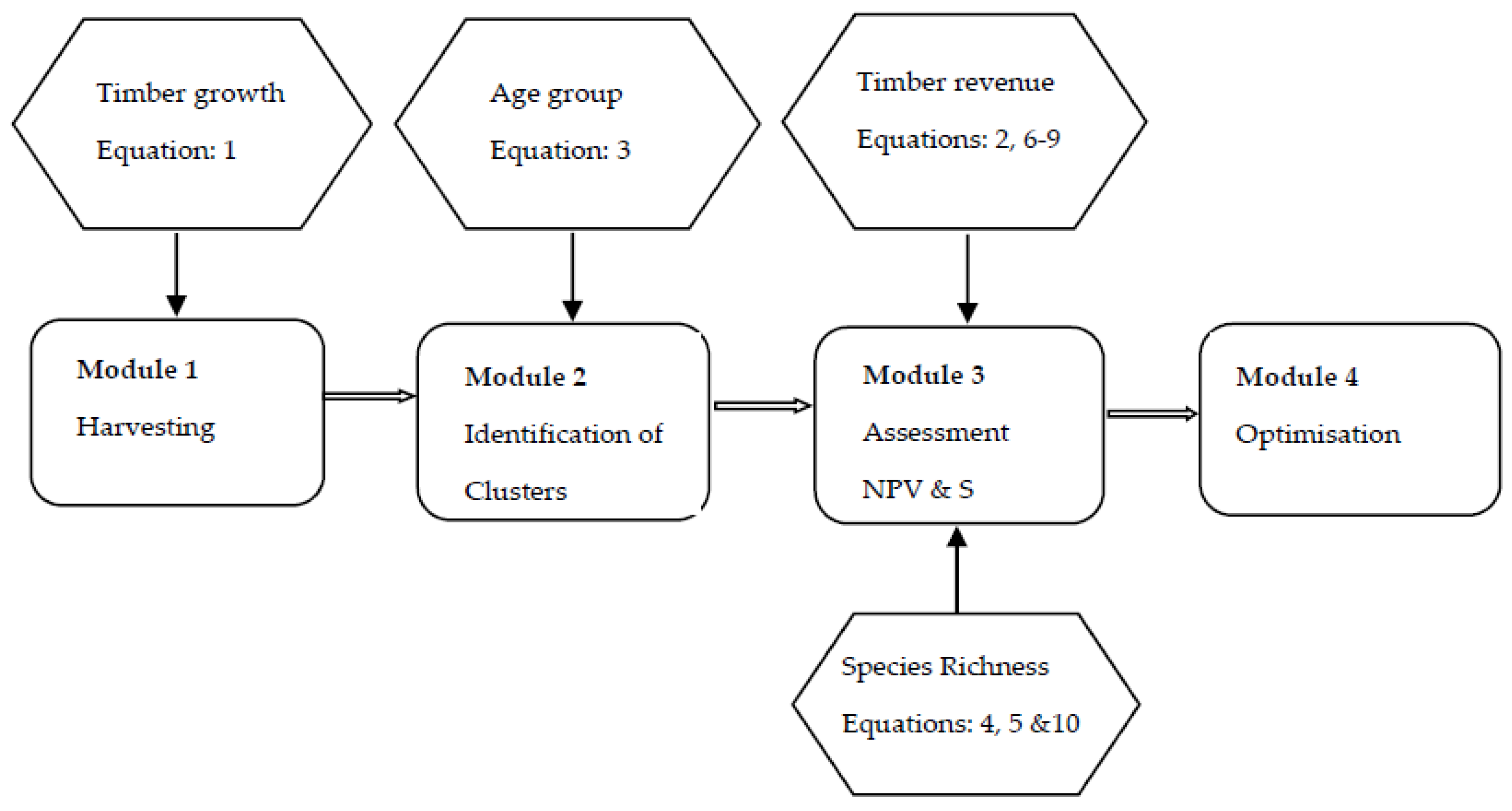
Figure 1 presents the model structure with four modules to decide cutting area and volume, identify clusters, assess profitability and species richness, and find an optimal strategy.

• Module 1: Involved calculating timber growth and a decision to cut or keep a stand in period t. The decisions to cut a stand vary with alternative management strategies. We let t run from 0 to T, and calculated timber volume based on Equations (1), (2), and (8).
• Module 2: Involved identifying clusters of clear-cutting area and of habitat area. We ran through stand 1 to stand n × n, ascertained whether $d_{ijt}=1$ (i.e., cut) or $x_{ijt}\ge A$ (i.e., habitat for plant species), and checked whether its adjacent stands are cut or aged older than A. If satisfied, clusters of clear cutting or habitat were recorded.
• Module 3: Involved calculating the NPV using Equations (6)–(9) and counting the number of species by applying Equations (5) and (10).
• Module 4: Involved all scenarios with different rotation ages being compared based on the objective variable. Then, the scenario that achieved the highest value of the NPV was chosen as the optimal management strategy in terms of timber extraction. The associated NPV and rotation length were referred to as NPV* and T*.

We applied this model according to clear-cutting and patch-clear-cutting strategies in order to analyse the trade-off between the economies of cutting scale and species richness.

In the clear-cutting strategy, a forest manager seeks to maximise the NPV from selling timber and ignores the impacts of this decision on the enhancement of plant species richness. To take advantage of the economies of scale (i.e., the larger the cutting area, the smaller the harvesting cost per ha) the forest manager cuts all the stands after T* years. The model of this strategy includes Equations (1)–(9). A stand is harvested ($d_{ijt}=1$) when it reaches year T* (Module 1). The optimal management strategy is denoted by $NP{V}_c^{*}$, $T_c^{*}$, and $S_c^{*}$.

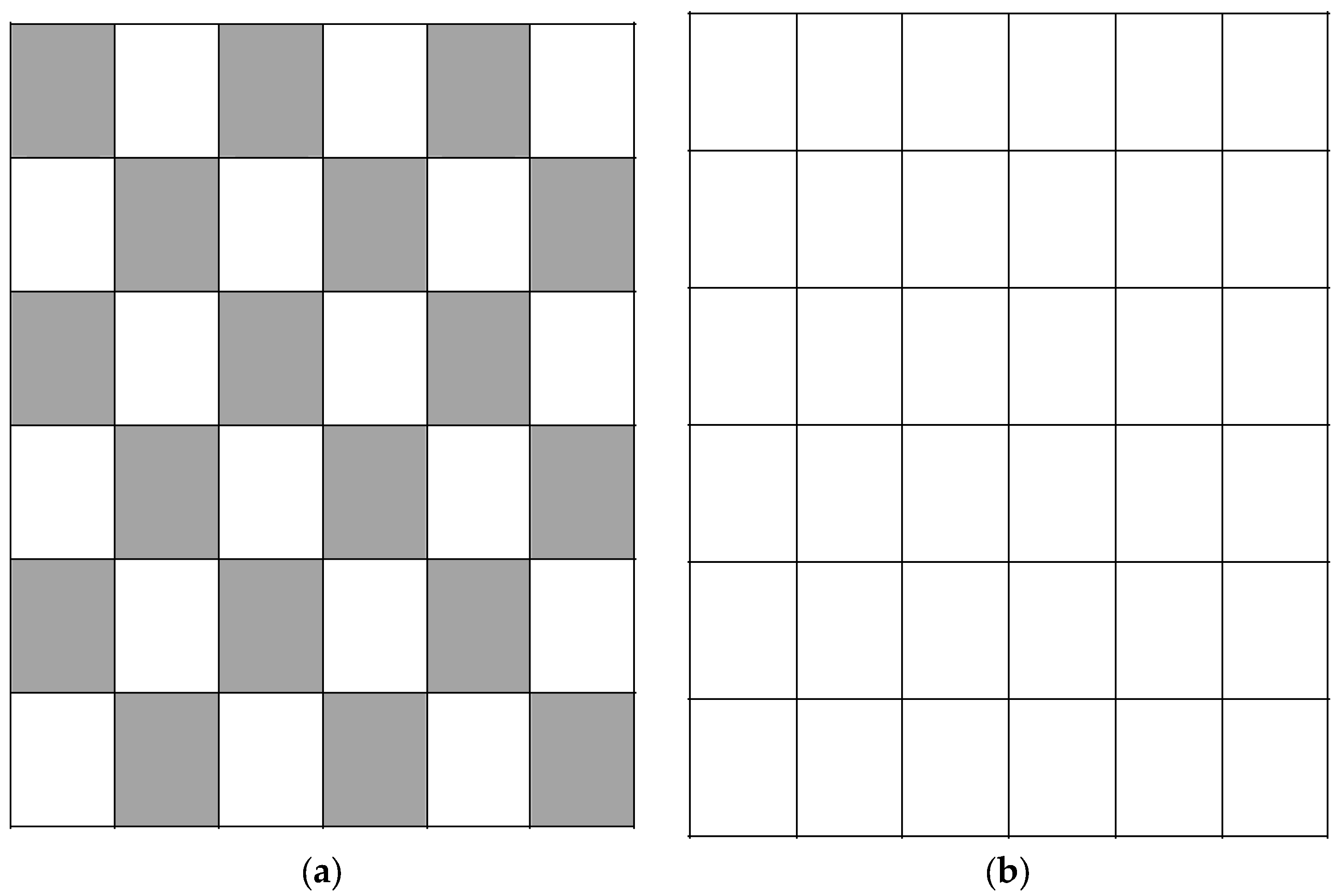
In the patch-clear-cutting strategy, the forest manager’s objective is to maximise the NPV from timber production but also to promote biodiversity by applying a small clear-cut size. In this strategy, the manager cuts a stand when it reaches T* years without cutting adjacent stands occurring at the same time (see Figure 2a,b). This strategy allows clear-cutting areas to be as fragmented as possible in order to increase landscape heterogeneity. This would help to promote conservation values through variation in the range of age classes of stands and the spatial juxtaposition of stands of different types and ages [36]. The model of this strategy includes Equations (1)–(10). In Module 1, a stand can be cut $d_{ijt}=1$ when it reaches year T* or beyond and $d_{i-1jt}=0$ and $d_{i+1jt}=0$ and $d_{ij-1t}=0$ and $d_{ij+1t}=0$. The optimal management strategy is denoted by $NP{V}_c^{*}$, $T_c^{*}$, and $S_c^{*}$.

The opportunity cost (OC) of increasing biodiversity via using a patch-clear-cutting strategy (over a clear-cutting strategy) is defined as the difference in the NPV between the two approaches. Therefore, it is the amount of money foregone when the patch-clear-cutting strategy is applied and a certain level of additional biodiversity is achieved as follows:

$$OC=\frac{NP{V}_c^{*}-NP{V}_P^{*}}{S_P^{*}-S_c^{*}}$$

(11)

This model (i.e., Equations (1)–(11)) was used to estimate the opportunity cost of plant diversity in New Zealand Pinus radiata plantation forests in the next section.

2.2. A Case Study of Pinus radiata in New Zealand

New Zealand is one of 25 global biodiversity hotspots [37] and yet plantation forests are common (at 7% and 22% of land surface and of total forest area, respectively [38]). As a result, the New Zealand forestry sector contributes 3.4% to annual GDP [39] and is the third largest export industry in New Zealand [38]. In 2007, approximately 19.3 million m³ of round wood were harvested, of which, 19.0 million m³ came from the clear felling of 43,000 hectares of plantation forests [40].

In New Zealand, exotic forests are planted for production purposes only [41]. However, plantation forests are further incentivised because of the potential of such forests to sequester carbon emissions from other sectors [42]. Forestry was the first sector to enter New Zealand’s Emission Trading Scheme (ETS), effective from 1 January 2008. This allows new forest plantations to earn carbon credits through the Kyoto Protocol. Plantation forests could also be promoted as supplying other ecosystem services, such as the maintenance of clean water, erosion control, and habitat provision [43]. Currently, exotic trees are the main crops in New Zealand, of which, 89% is Pinus radiata [40]. Pinus radiata was introduced into New Zealand in the 1840s and grows faster here than in any other country, with the typical rotation length being around 28 years [38].

Since clear cutting is popular and preserving biodiversity is becoming important in New Zealand plantations, this study applies the model described in the previous section to find the opportunity cost of conserving understorey plants in P. radiata forests. In the baseline scenario, we did not put any restriction on stand age that creates a favourable habitat for any particular species. However, in sensitivity analyses, we varied this stand age according to species re-colonisation or habitats for indigenous plant species.

For the P. radiata growth function, we used age and total standing volume from yield tables for Central North Island [44] since this area is the major plantation area in New Zealand [45]. The growth data are detailed in Appendix A.

The harvesting cost was obtained from an established database [46,47] with some adjustments, as detailed in Appendix B.

$$c=42.9y^{-0.118}, R^2=0.9$$

(12)

where c is the clear-cutting cost (expressed in NZD m⁻³) and y is the cutting area or the stand size (ha).

In Equation (12), β = 42.9 > 0 and η = −0.118. The cost function implies a decreasing marginal cost with the cutting area. Since $y\ge 0$, the first derivative $c_y^{\prime }<0$, hence (12) is a decreasing function. Therefore, the larger the cutting size, the less expensive the cutting cost m⁻³.

We assumed timber prices varied by tree ages. Since there are no data for the timber prices which vary with the tree ages, we estimated a weighted timber price using the ratio of pulp and logs at each tree age calculated from an official yield table [44]. This ratio for each tree age was then used to weigh pulp prices and log prices to create the timber prices associated with the tree ages. We used an average pulp price of 51 NZD m⁻³ and an average log price of 135 NZD m⁻³ in 2011 [48]. These estimated timber prices are detailed in Appendix A.

Table 1. Parameters used in the model.

Parameters	Unit	Values	Sensitivity Analyses	Uncertainty Analyses
Forest harvest size (a)	ha	2	1.5–5	No
Total stand (n)	number	400	No	No
Time horizon (T)	year	100	No	No
Yield (q)	m3	See Appendix A	No	Normal distribution
Exponent of the species area curve (z)	numeric	0.3	0.15–0.32	No
Biodiversity age (A)	year	0	8–20	No
Cost exponent (η)	numeric	−0.118 (see Appendix B)	(−0.5)–(−0.2)	No
Price (p)	NZD	See Appendix A	No	Normal distribution
Discount rate (r)	rate	0.07	0–0.15	No

shows the parameters used in our baseline model. We chose z = 0.3 in our baseline scenario since the species–area relationship for native forest remnants in New Zealand was assigned with z = 0.4 [49]. The quality of plantation forest habitat is lower than that of the native remnants (i.e., more disturbance), and thus can affect the dispersal of the native species. Moreover, we assumed a forest size of 400 stands to be sufficient to apply a patch-clear-cutting practice, and that the forest would exist over a 100-year time horizon, as in the literature [18,19]. We used a maximum rotation age for P. radiata of 40 years, as similar to the age listed in the yield table [44]. We also ran simulations with a maximum rotation age of 60 years but the optimal age solution was always less than 40 years, thus we used 40 years to reduce the computational time in uncertainty analyses. The discount rate of 7% (in real terms) was used as this is the rate that is mainly used in forest valuations in New Zealand [50].

2.3. Sensitivity and Uncertainty Analyses

We performed a sensitivity analysis of the opportunity cost with five parameters: discount rate (r), the exponent of species–area curve (z), the exponent of cutting cost (η), the size of forest stands (a), and stand age that creates favourable habitats (A) (see Table 1). Following Roy et al. [35], we assumed the number of associated plant species follows a species–area relationship. Based on Ogden et al. [51] and Brockerhoff et al. [6], we adopted stand age A which creates favourable conditions as being between one and 20 years. We also performed a sensitivity analysis to the cutting strategy (that is, a sustainable management scenario) by applying a sustainable cutting restriction so that the number of stands harvested was the same each year. This ensures a sustainable income from the forest and a sustainable quantity of timber supplied. It also creates a forest with a mixture of young, mature, and old forest stands that could be a habitat for a wide range of plant species.

We assumed timber yield followed a normal distribution with a standard deviation (SD). The SDs (see Appendix A) were derived from the yield table [52] based on timber volumes over different management strategies (i.e., production with and without thinning). We assumed timber price followed a normal distribution with a SD of 20% of the point estimate (see Appendix A). We ran 2000 iterations in the General Algebraic Modeling System (GAMS 23.6.5) [53]. There is no consensus in the literature regarding how many iterations are enough to guarantee a model convergence. A number of iterations as small as a few hundred has been applied in the forestry literature [54,55].

3. Results

In the baseline scenario, the optimal rotation age in the clear-cutting strategy was 24 years, a year shorter than that in the patch-clear-cutting strategy (

Table 2. Optimal rotations (T*), species richness (S*), and net present value (NPV*) from the baseline model and sensitivity analyses for Pinus radiata plantation forests in New Zealand.

Scenarios	Patch-Clear-Cutting Strategy (P)			Clear-Cutting Strategy (C)			Differences (P–C)			OC ($) Per Extra Species
	S* (Species·ha−1)	T* (Year)	NPV* ($·ha−1)	S*	T*	NPV*	∆S*	∆T*	∆NPV* (OC $·ha−1)	∆NPV*/∆S*
Baseline	59	25	7020	11	24	8157	48	1	−1137	24
Varying the discount rate
r = 0	60	33	136,954	12	33	157,473	48	0	−20,519	429
r = 0.03	59	26	26,894	12	26	31,064	47	0	−4170	88
r = 0.1	58	19	3493	12	19	4098	47	0	−605	13
r = 0.15	58	17	1396	12	16	1651	46	1	−255	5

Note: OC is the opportunity cost.

). It is also four years shorter than the usual 28-year rotation commonly used in New Zealand (with a range of 25 to 35 years) [56]. Species richness was substantially enhanced with the patch-clear-cutting strategy vs. the clear-cutting strategy (59 vs. 11 species, respectively, up to a maximal difference of 72 to 11 species). The clear-cutting strategy, however, was more financially rewarding than the patch-clear-cutting strategy with a gap of 1137 NZD·ha⁻¹ (14%) of the total forest. As such, the opportunity cost for obtaining one extra species of understorey plant in a plantation forest was 24 NZD on average. Figure 3 represents the trade-off between the number of understorey plant species and the NPV in the clear-cutting and patch-clear-cutting strategies. It is clear that the trade-offs begin to happen at a much higher species number (around 20 species) for patch-clear-cutting.

Sensitivity analyses suggested that the NPV and hence the opportunity cost were very sensitive to discount rates (Table 2). The NPV varied between 255 and 20,519 NZD·ha⁻¹, and therefore made the opportunity cost per extra species range from 5 to 429 NZD. The optimal rotation age was also sensitive to discount rates, and was between 16 and 33 years. However, there was only a slight difference (one year at most) in the optimal rotation ages between the two cutting strategies. Species richness was not very sensitive to discount rates as expected.

When cutting size was varied between 1.5 and 5 ha, the optimal rotation age remained the same for the clear-cutting strategy (24 years) and the patch-clear-cutting strategy (25 years). Species richness increased significantly, ranging from 31 to 72 species·ha⁻¹, in the patch-clear-cutting strategy. There was a trade-off between species richness and the NPV as the NPV reduced from 7490 to 6861 NZD·ha⁻¹ in this strategy. As a result, the difference in the NPV between the two cutting strategies ranged from 666 to 1295 NZD·ha⁻¹. The opportunity cost, in this case, did not vary in the same direction as the NPV did with regard to the cutting size. The opportunity cost decreased from 33 to 21 NZD·species⁻¹ as the cutting size decreased from 5 to 1.5 ha. That is, the latter was the optimal stand size for a forestry manager to adopt in terms of low cost per extra species gained (Figure 4a).

The opportunity cost was not sensitive to the exponent of the species–area curve. It varied between 23 and 24 NZD per extra species as the exponent increased from 0.15 to 0.32 (see Appendix C). The higher the exponent, the larger the number of species in plantation forests (between 53 and 60 species for the patch-clear-cutting strategy). An increase in the exponent of the species–area curve in this case could be a higher level of stand age heterogeneity or an older growth forest.

The opportunity cost (Figure 4b) increased disproportionately from 24 to 111 NZD per extra species as the favourable stand age (A) increased from 0 to 20 years. Species richness decreased significantly with an increase in A, ranging from 12 to 41 species·ha⁻¹ in the patch-clear-cutting strategy and from 2 to 8 species·ha⁻¹ in the clear-cutting strategy. The opportunity cost increased at a slower rate as the economies of scale of the harvesting went down (Figure 4c). The optimal rotation age for the clear-cutting strategy (20 years) was five years shorter than that of the baseline scenario.

In the sustainable management scenario, the optimal rotation age varied between 17 and 35 years (Figure 4d). It is noted that this is a minimum cutting age, so that it helps to create a forest with a mixture of young, mature, and old forest stands that could be a habitat for a wide range of plant species. Putting an age restriction on delaying the harvesting for understorey plant species that prefer old growth forests increased the opportunity cost sharply from 34 to 150 NZD per extra species.

Timber price and growth uncertainty analyses for optimal rotation and biodiversity of plantation forests in New Zealand are presented in

Table 3. Timber price and growth uncertainty analyses for optimal rotation and biodiversity of Pinus radiata plantations in New Zealand.

Scenarios	Patch-Clear-Cutting (P)			Clear-Cutting (C)			Differences (P − C)			OC ($) Per Extra Species ∆NPV*/∆S*
	S* (Species·ha−1)	T* (Year)	NPV* ($·ha−1)	S*	T*	NPV*	∆S*	∆T*	∆NPV* (OC $·ha−1)
Mean	58.59	22.5	10,103	11.68	22.1	11,362	46.90	0.4	−1258	27
Median	58.48	23.0	9985	11.67	22.0	11,239	46.81	1.0	−1257	27
Lower 95% SI	57.25	15.0	7875	11.42	15.0	8940	45.83	0.0	−1066	23
Upper 95% SI	59.4	32.0	13,276	11.79	31.0	14,747	47.61	1.0	−1471	31

Notes: T* is optimal rotations, S* is species richness, and NPV* is net present value.

. The mean species richness was 58.6 species·ha⁻¹ (95% confidence interval (CI): 57.2–59.4 species·ha⁻¹) for the patch-clear-cutting strategy, and was 11.7 species·ha⁻¹ (95% CI: 11.4–11.8 species·ha⁻¹) for the clear-cutting practice. The mean optimal rotation age for both strategies was about 22 years, with the patch-clear-cutting being one year wider in magnitude (95% CI: 15–32 years vs. 15–31 years). The mean NPVs were 10,103 and 11,362 NZD for the patch-clear-cutting and clear-cutting, respectively. The opportunity cost was therefore 27 NZD per extra species (95% CI: 23–31 NZD per extra species).

4. Discussion

In a time of rapid climate change, biodiversity conservation in production plantations has been called for in order to prevent accelerated loss of biodiversity [26]. This study analysed the benefits to biodiversity and the opportunity cost of adopting a patch-clear-cutting strategy over a clear-cutting strategy for managing P. radiata plantation forests. Assuming that forest stands at a certain age can generate a suitable habitat for plant species, the dynamics of species richness follows a power–law relation with the habitat area. The ecological-economic model therefore implies the higher the level of heterogeneity in the distribution of stands with different age classes, the higher the species richness, and the smaller the NPV.

The results suggest substantial biodiversity benefits from the patch-clear-cutting strategy over the clear-cutting strategy for understorey plant species (i.e., 59 vs. 11 species·ha⁻¹). However, the opportunity cost was non-trivial at 1260 NZD·ha⁻¹ (822 USD·ha⁻¹). This opportunity cost ha⁻¹ was close to an estimate of environmental values for plantation forests in New Zealand (900 NZD·ha⁻¹) using choice modelling [57]. Our finding about the opportunity cost was also in line with the finding [13,58] that the patch-clear-cutting strategy enhances biodiversity but lowers financial returns. Yet the difference in optimal rotation ages between the two cutting strategies was small (i.e., about one year), suggesting that forest managers would not need to delay cutting in order to enhance biodiversity through the patch-clear-cutting strategy. It is stressed that our estimated opportunity cost may only represent a limited portion of biodiversity value. In the case that the NPV is negative, forest owners would abandon the forests, and therefore there is no opportunity cost of biodiversity.

Furthermore, the opportunity cost decreased with a decrease in the patch-clear-cutting size. That is because when patch-clear-cutting size was reduced, the species richness increased and the timber revenue decreased, but at a slower rate. Our sensitivity analysis results suggested that the opportunity cost was very sensitive to the discount rate, an important factor in environment and ecosystem valuation [59,60,61]. Thus, there was a large difference in the opportunity cost from using a social discount rate (a low or even zero discount rate) and a private discount rate (a high discount rate) (see [61,62,63] for a discussion of social discount rate). The results also implied that it was very costly to enhance the value of plant species in mature and old growth forests. The scenario analysis indicated that there was a trade-off between sustainable management and timber revenue. It is relatively expensive to create a plantation forest with a mixture of young, mature, and old forest stands, which support the forest structure diversity (and hence plant species diversity).

The model developed in our study can potentially be applied to other types of forests and in other parts of the world. However, species–area relation parameters, cost parameters, timber prices, and growth parameters would need to be adapted. The results of this particular model are probably most transferable to plantation forests in temperate parts of countries such as Chile and Australia since P. radiata is also a major exotic tree species grown in these countries [9].

In the last half century, about 60% of all ecosystem services have declined [64]. One reason for this is that the benefits of ecosystems, such as watershed protection and habitat provision, have not been an integral part of the formal economic system. Paying for ecosystem services has been applied in some countries, such as Costa Rica, the United States, and South Africa among others [65,66,67]. For habitat provision, such as the one generated by using a patch-clear-cutting strategy in our study, it has been suggested that funding is via direct payment to achieve the socially optimal level of provision [68]. The opportunity costs reported in our study could, therefore, be considered as means to inform the appropriate payment level to promote biodiversity in plantation forests. In some cases, however, national policy makers may also wish to consider carbon sequestration associated with different forestry practices. At national and local levels, policy makers might also wish to reduce erosion and flood risk and improve fresh water quality in all plantation forests or particular watersheds. In such cases, they might wish to pay private foresters even more to change forestry practices (or else buy up forests for the government or even pass laws that require a certain type of forest management). Indeed, some Regional Councils in New Zealand have required certain harvesting strategies to protect against flood risk [69].

These results could also have an implication for implementing the Reducing Emissions from Deforestation and Forest Degradation (REDD+) mechanism, which considers the role of conservation, sustainable management of forests, and enhancement of forest carbon stocks. The REDD+ mechanism has been suggested both to be an effective tool for climate change mitigation (via carbon sequestration) and to offer the important co-benefits of biodiversity conservation [70].

In our study, only timber values were considered in the calculation of the opportunity cost, other values such as carbon sequestration, watershed protection, soil preservation, and water quality benefits, among others, have been ignored [71,72]. If these values were added, then the patch-clear-cutting strategy could become optimal from a both financial and biodiversity perspective (compared to the clear-cutting strategy).

In New Zealand, it has been known that specific management actions can benefit particular threatened species (e.g., clear-cutting edges provide foraging habitat for New Zealand falcons) [73]. Furthermore, it should be noted that the ability of a species to persist in the landscape depends on its metapopulation dynamics (i.e., by processes of colonization and extinction) [74]. There is evidence that the shape of the patches can affect the properties of the stand, such as increasing tree mortality with wind damage [75].

The composition of understorey species is very dependent on the geographic location of the forest and on the stage of plantation forest development. For example, new plantings on coastal sands will likely only have a very few species present, whereas forests on the central volcanic plateau may have a rich understorey of both exotic and indigenous species. In a recently planted P. radiata in the Kinleith Forest, Allen et al. [76] found up to 35 vascular plant species, 67% of which were indigenous. This level of species richness was greater than that for many New Zealand natural forests [76]. Ogden et al. [51] reported similar results from another Kinleith Forest study. This more recent study included a 67-year-old P. radiata forest, which had a fern understorey structure similar to that of native podocarp (Podocarpus spp.) and kauri (Agathis australis) forests.

We have not included the costs of fine-scale silvicultural managements such as site preparation (movement of wood debris, herbicide use, and soil mounding), pruning, stocking, and crop species selection (including mixtures). The cost functions involved some simplifying assumptions and ignored such aspects as: steepness of the forest, distance to the main road, size of trees, and types of cutting machinery (e.g., cable car or ground-based machines). Timber prices for different tree ages were based on the ratio of pulp and log prices. We did not take into account the fact that trees at the same age still produce slightly different log sizes as morphological differentiation between trees is a typical characteristic of any forest stand. However, the uncertainty arising from these limitations was shown in the timber price and growth uncertainty analyses.

5. Conclusions

This study shows the benefits to biodiversity, NPV, optimal rotation age, and also the opportunity cost associated with switching from a ‘business-as-usual’ forestry management system focused upon maximising timber extraction (clear-cutting) to a more biodiversity-friendly forest management system (patch clear-cutting). Our research can inform local decision making (e.g., financial compensation to foresters or laws on cutting strategies by local or national governments in priority areas for conservation or in flood-prone watersheds), however, such work may also inform international systems of payments for environmental services (e.g., via the REDD+ mechanism) to conserve biodiversity in developing countries with plantation forests involving P. radiata or other plantation species.

References

1. Costanza, R.; D’Arge, R.; de Groot, R.; Farber, S.; Grasso, M.; Hannon, B.; Limburg, K.; Naeem, S.; O’Neill, R.V.; Paruelo, J.; et al. The value of the world’s ecosystem services and natural capital. Nature 1997, 387, 253–260. [Google Scholar] [CrossRef]
2. Hassan, R.M.; Scholes, R.; Ash, N. Ecosystems and human well-being: Current state and trends. In The Millennium Ecosystem Assessment; Island Press: Washington, DC, USA, 2005; Volume 1, p. 23. [Google Scholar]
3. Brockerhoff, E.G.; Ecroyd, C.E.; Leckie, A.C.; Kimberley, M.O. Diversity and succession of adventive and indigenous vascular understorey plants in Pinus radiata plantation forests in New Zealand. For. Ecol. Manag. 2003, 185, 307–326. [Google Scholar] [CrossRef]
4. Laurance, W.F. Have we overstated the tropical biodiversity crisis? Trends Ecol. Evol. 2007, 22, 65–70. [Google Scholar] [CrossRef] [PubMed]
5. Food and Agriculture Organization of the United Nations (FAO). State of the World’s Forests 2007; Food and Agriculture Organization of the United Nations: Rome, Italy, 2007. [Google Scholar]
6. Brockerhoff, E.G.; Jactel, H.; Parrotta, J.A.; Quine, C.P.; Sayer, J. Plantation forests and biodiversity: Oxymoron or opportunity? Biodivers. Conserv. 2008, 17, 925–951. [Google Scholar] [CrossRef]
7. Barlow, J.; Gardner, T.A.; Araujo, I.S.; Ávila-Pires, T.C.; Bonaldo, A.B.; Costa, J.E.; Esposito, M.C.; Ferreira, L.V.; Hawes, J.; Hernandez, M.I.M.; et al. Quantifying the biodiversity value of tropical primary, secondary, and plantation forests. Proc. Natl. Acad. Sci. USA 2007, 104, 18555–18560. [Google Scholar] [CrossRef] [PubMed]
8. Nyland, R.D. Silviculture: Concepts and Applications, 2nd ed.; McGraw-Hill Higher Education: New York, NY, USA, 2002; p. 704. [Google Scholar]
9. Hagner, S. Forest Management in Temperate and Boreal Borests: Current Practices and the Scope for Implementing Sustainable Forest Management; Working Paper: Fao/fpirs/03; Food and Agriculture Organization of the United Nations (FAO), Forestry Policy and Planning Division: Rome, Italy, 1999; p. 47. [Google Scholar]
10. Maclaren, J.P. Environmental Effects of Planted Forests in New Zealand: The Implications of Continued Afforestation of Pasture; New Zealand Forest Research Institute: Rotorua, New Zealand, 1996; Volume 198, p. 180. [Google Scholar]
11. Applegate, G.; Putz, F.E.; Snook, L.K. Who Pays for and Who Benefits from Improved Timber Harvesting Practices in the Tropics? Lessons Learned and Information Gaps; Center for International Forestry Research: Jakarta, Indonesia, 2004; p. 35. [Google Scholar]
12. Nasi, R.; Putz, F.E.; Pacheco, P.; Wunder, S.; Anta, S. Sustainable forest management and carbon in tropical latin america: The case for redd+. Forests 2011, 2, 200–217. [Google Scholar] [CrossRef]
13. Lindenmayer, D.B.; Hobbs, R.J. Fauna conservation in australian plantation forests—A review. Biol. Conserv. 2004, 119, 151–168. [Google Scholar] [CrossRef]
14. Maynard, D.G.; MacIsaac, D.A. Soil nutrient and vegetation response to patch clear-cutting of an aspen forest near Meadow Lake, Saskatchewan. Can. J. Soil Sci. 1998, 78, 59–68. [Google Scholar] [CrossRef]
15. Torras, O.; Saura, S. Effects of silvicultural treatments on forest biodiversity indicators in the Mediterranean. For. Ecol. Manag. 2008, 255, 3322–3330. [Google Scholar] [CrossRef]
16. Pawson, S.; Brockerhoff, E.; Didham, R.; Norton, D. Clearfell harvest size: A key issue for biodiversity conservation in New Zealand’s plantation forests. N. Z. J. For. 2005, 50, 29–32. [Google Scholar]
17. Nguyen, T.T.; Nghiem, N. Optimal forest rotation for carbon sequestration and biodiversity conservation by farm income levels. For. Policy Econ. 2016, 73, 185–194. [Google Scholar] [CrossRef]
18. Calkin, D.E.; Montgomery, C.A.; Schumaker, N.H.; Polasky, S.; Arthur, J.L.; Nalle, D.J. Developing a production possibility set of wildlife species persistence and timber harvest value. Can. J. For. Res. 2002, 32, 1329–1342. [Google Scholar] [CrossRef]
19. Hurme, E.; Kurttila, M.; Monkkonen, M.; Heinonen, T.; Pukkala, T. Maintenance of flying squirrel habitat and timber harvest: A site-specific spatial model in forest planning calculations. Landsc. Ecol. 2007, 22, 243–256. [Google Scholar] [CrossRef]
20. Loomis, J.B.; White, D.S. Economic benefits of rare and endangered species: Summary and meta-analysis. Ecol. Econ. 1996, 18, 197–206. [Google Scholar] [CrossRef]
21. Bann, C. An overview of valuation techniques: Advantages and limitations. Asean Biodivers. 2002, 2, 8–16. [Google Scholar]
22. Martin-Lopez, B.; Montes, C.; Benayas, J. Economic valuation of biodiversity conservation: The meaning of numbers. Conserv. Biol. 2008, 22, 624–635. [Google Scholar] [CrossRef] [PubMed]
23. Bandara, R.; Tisdell, C. Comparison of rural and urban attitudes to the conservation of Asian elephants in Sri Lanka: Empirical evidence. Biol. Conserv. 2003, 110, 327–342. [Google Scholar] [CrossRef]
24. Eiswerth, M.E.; Van Kooten, G.C. The ghost of extinction: Preservation values and minimum viable population in wildlife models. Ecol. Econ. 2009, 68, 2129–2136. [Google Scholar] [CrossRef]
25. Nghiem, T.H.N. Optimal Forest Management for Carbon Sequestration and Biodiversity Maintenance. Ph.D. Thesis, Massey University, Manawatu, New Zealand, 2011. [Google Scholar]
26. Convention on Biological Diversity. Forest Biological Diversity. Available online: http://www.cbd.int/decisions/cop-06.shtml?m=COP-06&id=7196&lg=0 (accessed on 25 September 2007).
27. Nghiem, N. Optimal forest management for timber value and carbon sequestration benefits in tropical planted forests: A case study of household foresters in Vietnam. Environ. Dev. Econ. 2015, 20, 746–766. [Google Scholar] [CrossRef]
28. Nghiem, N. Optimal rotation age for carbon sequestration and biodiversity conservation in Vietnam. For. Policy Econ. 2014, 38, 56–64. [Google Scholar] [CrossRef]
29. Nghiem, N. Biodiversity conservation attitudes and policy tools for promoting biodiversity in tropical planted forests. Biodivers. Conserv. 2013, 22, 373–403. [Google Scholar] [CrossRef]
30. Woollons, R.; Whyte, A. Analysis of growth and yield from three kaingaroa thinning experiments. N. Z. For. 1989, 34, 12–15. [Google Scholar]
31. Keenan, R.; Lamb, D.; Woldring, O.; Irvine, T.; Jensen, R. Restoration of plant biodiversity beneath tropical tree plantations in northern australia. For. Ecol. Manag. 1997, 99, 117–131. [Google Scholar] [CrossRef]
32. Lugo, A.E. Comparison of tropical tree plantations with secondary forests of similar age. Ecol. Monogr. 1992, 62, 1–41. [Google Scholar] [CrossRef]
33. Munro, N.T.; Fischer, J.; Wood, J.; Lindenmayer, D.B. Revegetation in agricultural areas: The development of structural complexity and floristic diversity. Ecol. Appl. 2009, 19, 1197–1210. [Google Scholar] [CrossRef] [PubMed]
34. Bremer, L.L.; Farley, K.A. Does plantation forestry restore biodiversity or create green deserts? A synthesis of the effects of land-use transitions on plant species richness. Biodivers. Conserv. 2010, 19, 3893–3915. [Google Scholar] [CrossRef]
35. Preston, F.W. The canonical distribution of commonness and rarity: Part I. Ecology 1962, 43, 185–215. [Google Scholar] [CrossRef]
36. Roy, M.; Pascual, M.; Levin, S.A. Competitive coexistence in a dynamic landscape. Theor. Popul. Biol. 2004, 66, 341–353. [Google Scholar] [CrossRef] [PubMed]
37. Myers, N.; Mittermeier, R.A.; Mittermeier, C.G.; Fonseca, G.A.B.D.; Kent, J. Biodiversity hotspots for conservation priorities. Nature 2000, 403, 853–858. [Google Scholar] [CrossRef] [PubMed]
38. The New Zealand Forest Owners Association. New Zealand Plantation Forestry. Available online: http://www.nzfoa.org.nz/index.php?/Home/New_Zealand_plantation_forestry (accessed on 29 January 2009).
39. Ministry of Agriculture and Forestry. New Zealand Forest Industry Facts & Figures 2007/2008. Available online: http://www.maf.govt.nz/statistics/forestry/other-forestry-releases/facts-figures/ (accessed on 29 January 2009).
40. Ministry of Agriculture and Forestry. A National Exotic Forest Description 2007. Available online: http://www.maf.govt.nz/mafnet/publications/nefd/national-exotic-forest-2007/index.htm (accessed on 29 January 2009).
41. Food and Agriculture Organization of the United Nations (FAO). Global Forest Resources Assessment 2005; Food and Agriculture Organization of the United Nations: Rome, Italy, 2006. [Google Scholar]
42. Ministry of Agriculture and Forestry. Future Drivers for New Zealand Forestry. Available online: http://www.maf.govt.nz/forestry/publications/future-drivers/ (accessed on 21 January 2009).
43. Ausseil, A.G.E.; Dymond, J.R.; Kirschbaum, M.U.F.; Andrew, R.M.; Parfitt, R.L. Assessment of multiple ecosystem services in New Zealand at the catchment scale. Environ. Model. Softw. 2013, 43, 37–48. [Google Scholar] [CrossRef]
44. Ministry for Primary Industries. National Exotic Forest Regional Yield Tables. Available online: http://www.mpi.govt.nz/news-resources/statistics-forecasting/statistical-publications/nefd-regional-yield-tables.aspx (accessed on 22 October 2012).
45. Ministry of Agriculture and Forestry. Fact and Figure 2008/2009; Ministry of Agriculture and Forestry: Wellington, New Zealand, 2009.
46. Murphy, G. Functions to predict average piece size and average haul volume for New Zealand clearfell cable logging operations. N. Z. J. For. 1984, 29, 60–65. [Google Scholar]
47. Horgan, G. Financial Returns and Forestry Planting Rates; New Zealand Ministry of Agriculture and Forestry: Wellington, New Zealand, 2007.
48. Ministry for Primary Industries. Indicative New Zealand Radiata Pine Log Prices. Available online: http://www.mpi.govt.nz/news-resources/statistics-forecasting/forestry/indicative-new-zealand-radiata-pine-log-prices (accessed on 15 July 2012).
49. Dymond, J.R.; Ausseil, A.G.; Shepherd, J.D.; Janssen, H. A landscape approach for assessing the biodiversity value of indigenous forest remnants: Case study of the Manawatu/Wanganui region of New Zealand. Ecol. Econ. 2007, 64, 82–91. [Google Scholar] [CrossRef]
50. Manley, B. Discount rates used for forest valuation—Results of 2007 survey. N. Z. J. For. 2007, 52, 21–27. [Google Scholar]
51. Ogden, J.; Braggins, J.; Stretton, K.; Anderson, S. Plant species richness under Pinus radiata stands on the central North Island Volcanic Plateau, New Zealand. N. Z. J. Ecol. 1997, 21, 17–29. [Google Scholar]
52. Ministry of Forestry. National Exotic Forest Description Regional Yield Tables as at 1 April 1995; Ministry of Forestry: Wellington, New Zealand, 1996.
53. GAMS 23.6.5. Available online: http://www.gams.com/ (accessed on 5 November 2016).
54. Heath, L.S.; Smith, J.E. An assessment of uncertainty in forest carbon budget projections. Environ. Sci. Policy 2000, 3, 73–82. [Google Scholar] [CrossRef]
55. Eyvindson, K.; Kangas, A. Evaluating the required scenario set size for stochastic programming in forest management planning: Incorporating inventory and growth model uncertainty. Can. J. For. Res. 2015, 46, 340–347. [Google Scholar] [CrossRef]
56. Berg, P. Radiata Pine—Growing and Harvesting the Forest, TE Ara—The Encyclopedia of New Zealand. Available online: http://www.TeAra.govt.nz/en/radiata-pine/page-4 (accessed on 22 October 2016).
57. Rivas Palma, R.M. Environmental and Social Values from Plantation Forests: A Study in New Zealand with Focus on the Hawke’s Bay Region. Ph.D. Thesis, University of Canterbury, Christchurch, New Zealand, 2008. [Google Scholar]
58. Rüger, N.; Gutiérrez, Á.; Kissling, W.D.; Armesto, J.J.; Huth, A. Ecological impacts of different harvesting scenarios for temperate evergreen rain forest in southern chile—A simulation experiment. For. Ecol. Manag. 2007, 252, 52–66. [Google Scholar] [CrossRef]
59. Costanza, R.; Farber, S.C.; Maxwell, J. Valuation and management of wetland ecosystems. Ecol. Econ. 1989, 1, 335–361. [Google Scholar] [CrossRef]
60. Fisher, A.C.; Krutilla, J.V. Resource conservation, environmental preservation, and the rate of discount. Q. J. Econ. 1975, 89, 358–370. [Google Scholar] [CrossRef]
61. Howarth, R.B.; Norgaard, R.B. Intergenerational transfers and the social discount rate. Environ. Resour. Econ. 1993, 3, 337–358. [Google Scholar] [CrossRef]
62. Rambaud, S.C.; Torrecillas, M.J.M. Some considerations on the social discount rate. Environ. Sci. Policy 2005, 8, 343–355. [Google Scholar] [CrossRef]
63. Weitzman, M.L. On the “environmental” discount rate. J. Environ. Econ. Manag. 1994, 26, 200–209. [Google Scholar] [CrossRef]
64. Millennium Ecosystem Assessment. Ecosystems and Human Well-Being: General Synthesis; Island Press: Washington, DC, USA, 2005. [Google Scholar]
65. Milne, S.; Niesten, E. Direct payments for biodiversity conservation in developing countries: Practical insights for design and implementation. Oryx 2009, 43, 530–541. [Google Scholar] [CrossRef]
66. Turpie, J.K.; Marais, C.; Blignaut, J.N. The working for water programme: Evolution of a payments for ecosystem services mechanism that addresses both poverty and ecosystem service delivery in South Africa. Ecol. Econ. 2008, 65, 788–798. [Google Scholar] [CrossRef]
67. Madsen, B.; Carroll, N.; Brands, K.M. State of Biodiversity Markets: Offset and Compensation Programs Worldwide; Ecosystem Marketplace: Washington, DC, USA, 2010. [Google Scholar]
68. Kinzig, A.; Perrings, C.; Chapin, F., III; Polasky, S.; Smith, V.; Tilman, D.; Turner, B., II. Paying for ecosystem services—Promise and peril. Science 2011, 334, 603–604. [Google Scholar] [CrossRef] [PubMed]
69. Wellington Regional Council. Hutt River Floodplain Management Plan—For the Hutt River and Its Environment; Wellington Regional Council: Wellington, New Zealand, 2001.
70. Busch, J.; Godoy, F.; Turner, W.R.; Harvey, C.A. Biodiversity co-benefits of reducing emissions from deforestation under alternative reference levels and levels of finance. Conserv. Lett. 2011, 4, 101–115. [Google Scholar] [CrossRef]
71. Carnus, J.M.; Parrotta, J.; Brockerhoff, E.G.; Arbez, M.; Jactel, H.; Kremer, A.; Lamb, D.; O’Hara, K.; Walters, B. Planted forests and biodiversity. In IUFRO Occasional Paper; IUFRO: Vienna, Austria, 2003; pp. 31–50. [Google Scholar]
72. Evans, J. The multiple roles of planted forests. In Planted Forests. Uses, Impacts and Sustainability; CAB International and FAO: Wallingford, UK, 2009; pp. 61–90. [Google Scholar]
73. Seaton, R. The Ecological Requirements of the New Zealand Falcon (Falco novaeseelandiae) in Plantation Forestry. Ph.D. Thesis, Massey University, Palmerston North, New Zealand, 2007. [Google Scholar]
74. Hanski, I. Metapopulation dynamics. Nature 1998, 396, 41–49. [Google Scholar] [CrossRef]
75. Lindenmayer, D.; Franklin, J.F. Conserving Forest Biodiversity: A Comprehensive Multiscaled Approach, 2nd ed.; Island Press: Washington, DC, USA, 2002; p. 351. [Google Scholar]
76. Allen, R.B.; Platt, K.H.; Coker, R.E.J. Understorey species composition patterns in a Pinus radiata plantation on the central north island volcanic plateau, New Zealand. N. Z. J. For. Sci. 1995, 25, 301–317. [Google Scholar]
77. Terlesk, C.J. Harvesting: Pinus radiata production and cost trends. N. Z. J. For. 1980, 25, 172–183. [Google Scholar]
78. Long, A. Environmentally Sound Forest Harvesting; School of Forest Resources and Conservation, Florida Cooperative Extension Service, Institute of Food and Agricultural Sciences, University of Florida Gainesville: Gainesville, FL, USA, 1994; Volume SS-FOR-6, p. 11. [Google Scholar]
79. Ministry of Forestry. Small forest management. In Harvesting a Small Forest; Ministry of Forestry and New Zealand Logging Industry Research Organisation: Wellington, New Zealand, 1996; p. 39. [Google Scholar]
80. Dickson, A.; Bloomberg, M. An economic feasibility study of partial harvesting in a radiata pine plantation in canterbury, New Zealand. In Proceedings of the Conference Joint Australia and New Zealand Institute of Forestry, Queenstown, New Zealand, 27 April–1 May 2003; Mason, E., Perley, C., Eds.; Ministry of Agriculture and Forestry: Wellington, New Zealand, 2003; pp. 370–378. [Google Scholar]
81. Russell, F.; Mortimer, D. A Review of Small-Scale Harvesting Systems in Use Worldwide and Their Potential Application in Irish Forestry; COFORD: Dublin, Ireland, 2005; p. 48. [Google Scholar]
82. Zhang, Y.; Zhang, D.; Schelhas, J. Small-scale non-industrial private forest ownership in the United States: Rationale and implications for forest management. Silva Fenn. 2005, 39, 443–454. [Google Scholar] [CrossRef]
83. OECD. Key Short-Term Economic Indicators Metadata: Consumer Prices—Annual Inflation. Available online: http://stats.oecd.org/index.aspx?queryid=21761 (accessed on 15 June 2011).
84. Kantola, M. Role of Forestry in Small Farms. Unasylva 1967, 21. Available online: http://www.Fao.Org/docrep/59708e/59708e03.Htm (accessed on 5 November 2016). [Google Scholar]
Figure 1. Model structure showing four modules to decide “Forest harvest area and volume”, identify “clusters (connected stands)”, assess “profitability (timber Net Present Value (NPV))” and “species richness (S) for plant understorey”, and find an optimal strategy (see the text for details).
Forests 07 00297 g001
Figure 2. (a) Patch-clear-cutting strategy and (b) Clear-cutting strategy in the modelling. Each square represents a stand. The shaded squares are stands with standing trees, and white squares are harvested stands.
Forests 07 00297 g002
Figure 3. Trade-off between the number of understorey plant species conserved and the NPV for all the scenarios in the clear-cutting and patch-clear-cutting strategies in Pinus radiata plantation forests in New Zealand.
Forests 07 00297 g003
Figure 4. Sensitivity analyses on the opportunity cost (OC) per extra species between the patch-clear-cutting and clear-cutting strategies for Pinus radiata plantation forests in New Zealand with regards to stand size (a); stand age (b); economies of scale of the harvesting cost (c); and minimum harvesting age (d).
Forests 07 00297 g004