1. Introduction
Forests are one of Europe’s most important renewable resources, and provide multiple benefits to society and the economy. Providing information on the state and trends of forest resources is one of the most important challenges at a global level. Although a great deal of effort has been made for monitoring, assessing, and reporting on forest ecosystems [
1,
2], several challenges remain because forest cover is increasing, and, in addition, due to the national and international commitments to biodiversity conservation and renewable energy, which require even more information on forests and on Sustainable Forest Management (SFM). The current trend of afforestation and natural succession of abandoned lands [
3,
4] have increased the EU’s forest area by around 0.4% per year in recent decades [
5]. As a result, on the one hand, there is an increase of forest cover, while, on the other hand, there is a strong interest in assessing the productivity of forests and the trade-off between the production of wood and non-wood forest products, and other ecosystem services, derived from forest resources [
6]. For this reason, many efforts have been made in assessing the progress towards SFM, testing, implementing [
7,
8], and developing (see [
9]) new SFM indicators to enable the support of policy and decision makers, in order to discover strategies to foster forest resilience and adaptation to climate change.
Traditional inventories, based on field measurement, are the most direct way to estimate a forest biomass pool, and are considered statistically highly accurate. However, they are expensive, time consuming [
10], and difficult to implement (i.e., steeped, rocked, and ownership regimes hinder practical implementation). Furthermore, Andersen et al. [
11] highlighted that field samplings are (typically) based on a relatively limited inventory of stand attributes, and that they will be subject to sampling errors, and will be unable to capture variations in stand structure at fine spatial scales over the landscape.
In the last few decades, however, innovative tools and methodologies, such as airborne Light Detection And Ranging (LiDAR), also referred to as Airborne Laser Scanning (ALS), have been developed and implemented at local, landscape/watershed, and regional scales [
12,
13,
14]. Basically, LiDAR represents a powerful tool for deriving relevant forest inventory information; however, its derived products can never reveal certain tree patterns that are measured in the field, such as suppressed trees, grouped trees in dense forests, and understory [
15,
16,
17]. This is even more evident in the Mediterranean forest ecosystems [
18], where the complexity of forest structures, which are affected by, for example, the excessive fragmentation of ownership regimes, and the traditional forest management systems, make it more difficult to obtain realistic representation through ALS data of some forest components such as deadwood, suppressed trees, understory vegetation, and tree regeneration. On the other hand, use of LiDAR technologies have gained greater importance, not only for estimating forest attributes, but also for estimating the biomass pool of trees outside forests and for urban trees [
19,
20], which play an important role in the provision of ecosystem services.
One of the current challenges for forest researchers and forest decision makers is therefore to identify effective remote-based approach that enable proper estimation of the individual tree numbers, tree height, tree diameter, tree crown boundaries, spatial (i.e., vertical and horizontal) variability of plant density, biomass pool, carbon sequestration, and their changes over the years, in order of forest inventory as well as for defining the management strategies to better adapt to climate change. For this reason, several studies are focused on algorithm calibration and accuracy assessment [
19] within Area-Based Approaches (ABA) or Individual Tree Detection approaches (ITD). Recent studies report that the use of smoothed canopy height models [
21,
22], segmented laser point clouds [
23,
24], or hybrid techniques that combine the ALS data with different types of geo-data and a variety of a priori information [
25,
26] have produced encouraging results over coniferous forests, but similar performances have not been assessed for broadleaved woodlands or multi-layered forest canopies, which are characterized by complex plant morphology with overlapping crowns [
14,
27,
28]. Furthermore, most of these studies use a processed point cloud and so some information, which can be supportive to predict forest inventory variables, is lost by transforming the ALS data.
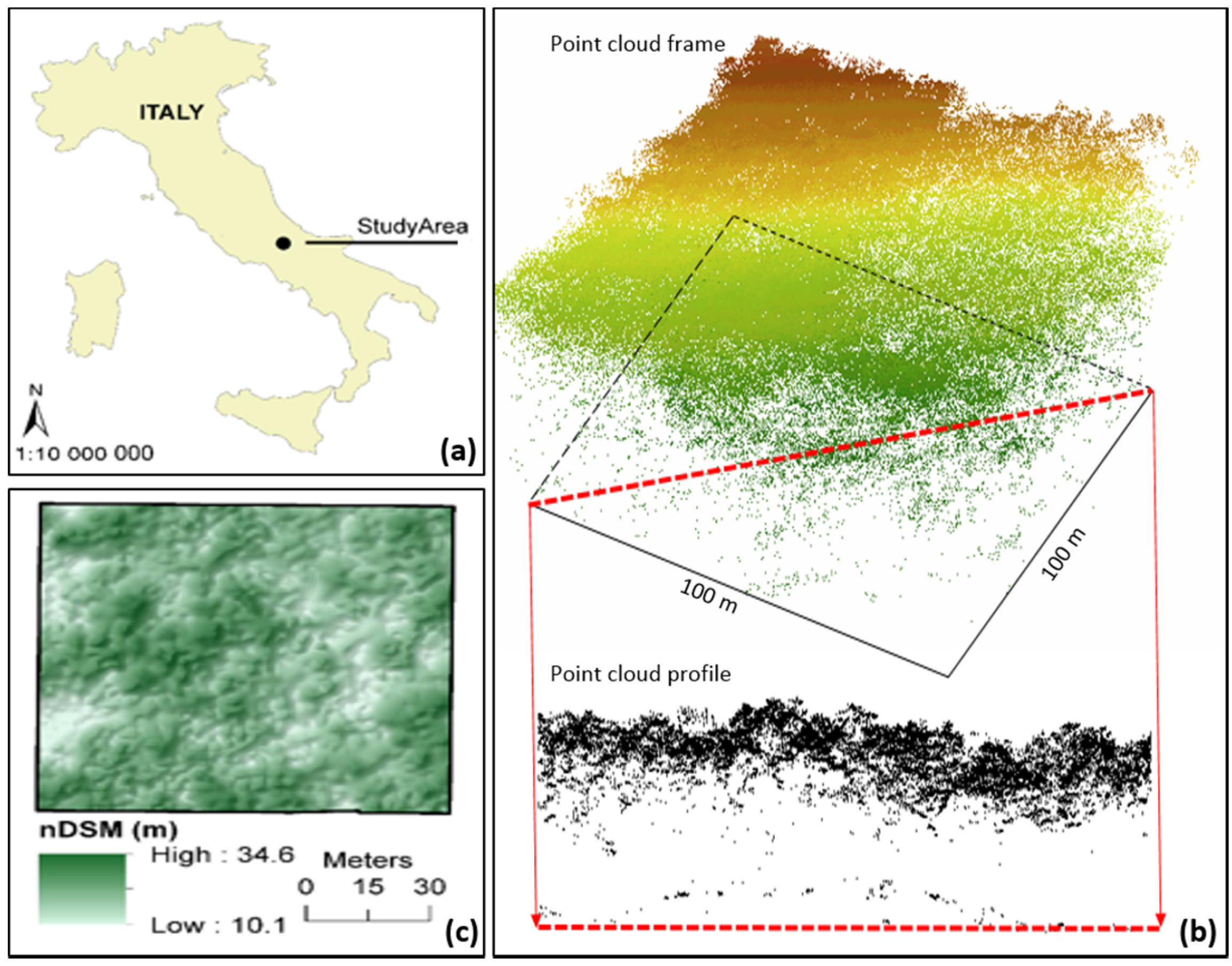
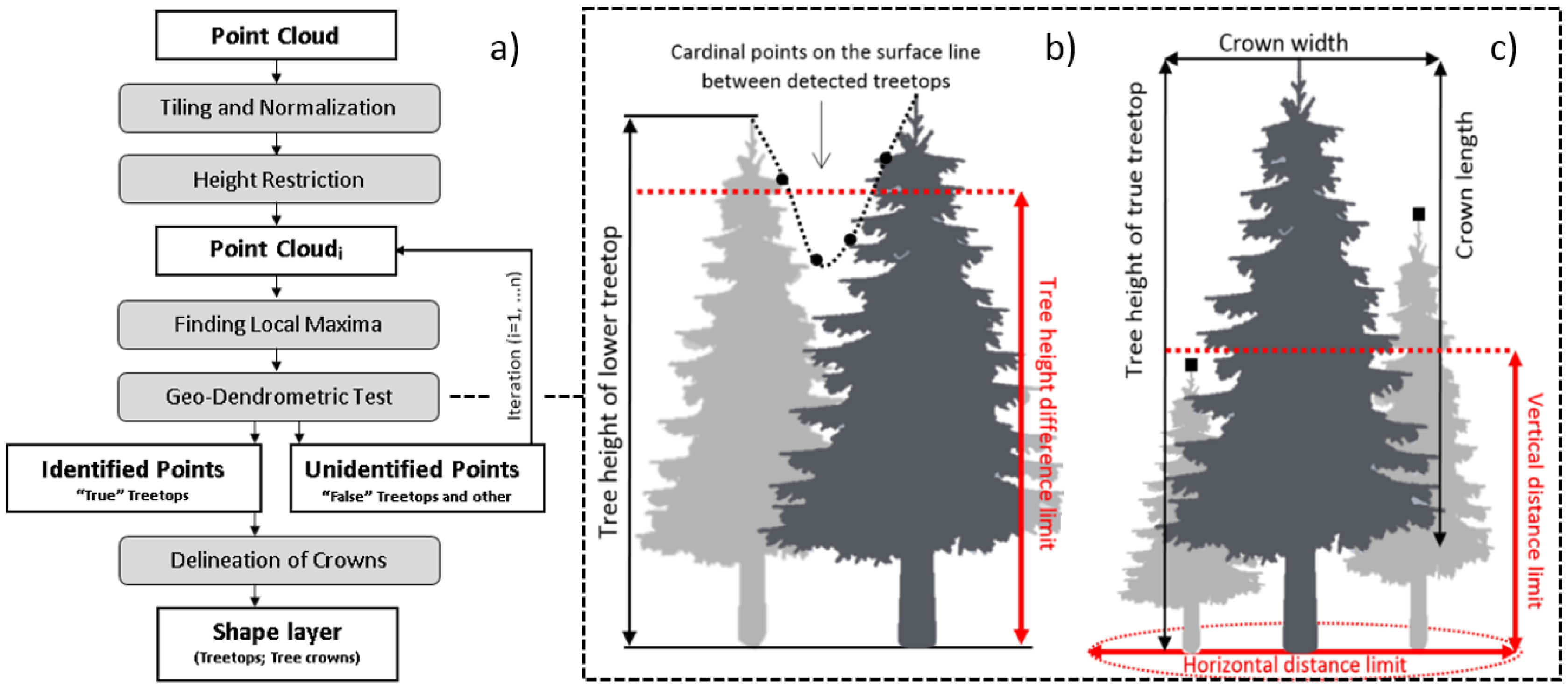
The purpose of this study is to assess the usability and accuracy of our own single-tree detection algorithm within remote-based forest inventory, using airborne LiDAR data acquired with a lightweight scanner in a selected type of Italy’s multilayered deciduous forest. Main forestry tree and stand characteristics, such as number of trees, tree height, tree diameter, and volume, were evaluated separately. We were particularly interested in identifying the benefits of the algorithm which uses the complete information contained in original ALS data in all procedures, and each iteration of single tree detection includes tests for treetops authenticity based on tree allometry rules. The following section reports the material and methods used to carry out the study.
Section 3 shows the results, followed by
Section 4 and
Section 5, which describe the discussion and conclusions, respectively.
3. Results
3.1. Accuracy of Tree Number Detection
The proportion of trees found in the sample plot was about 24%, 36%, and 48%, for all trees, trees higher than 16 m, and trees higher than 21 m, respectively. Selected height intervals (trees higher than 16 m and 21 m) related to the height variability of points in the point cloud (two and one standard deviation). Simultaneously, we found quite a low commission rate (false positive detection) of approximately 4%–9% (
Table 1).
As expected, the detection rate has a significant relationship with the social position of trees and dropped when trees were occluded by taller or bigger trees. The detection rates for dominant, codominant, intermediate, and suppressed trees are 66%, 48%, 18%, and 5%, respectively (
Table 2).
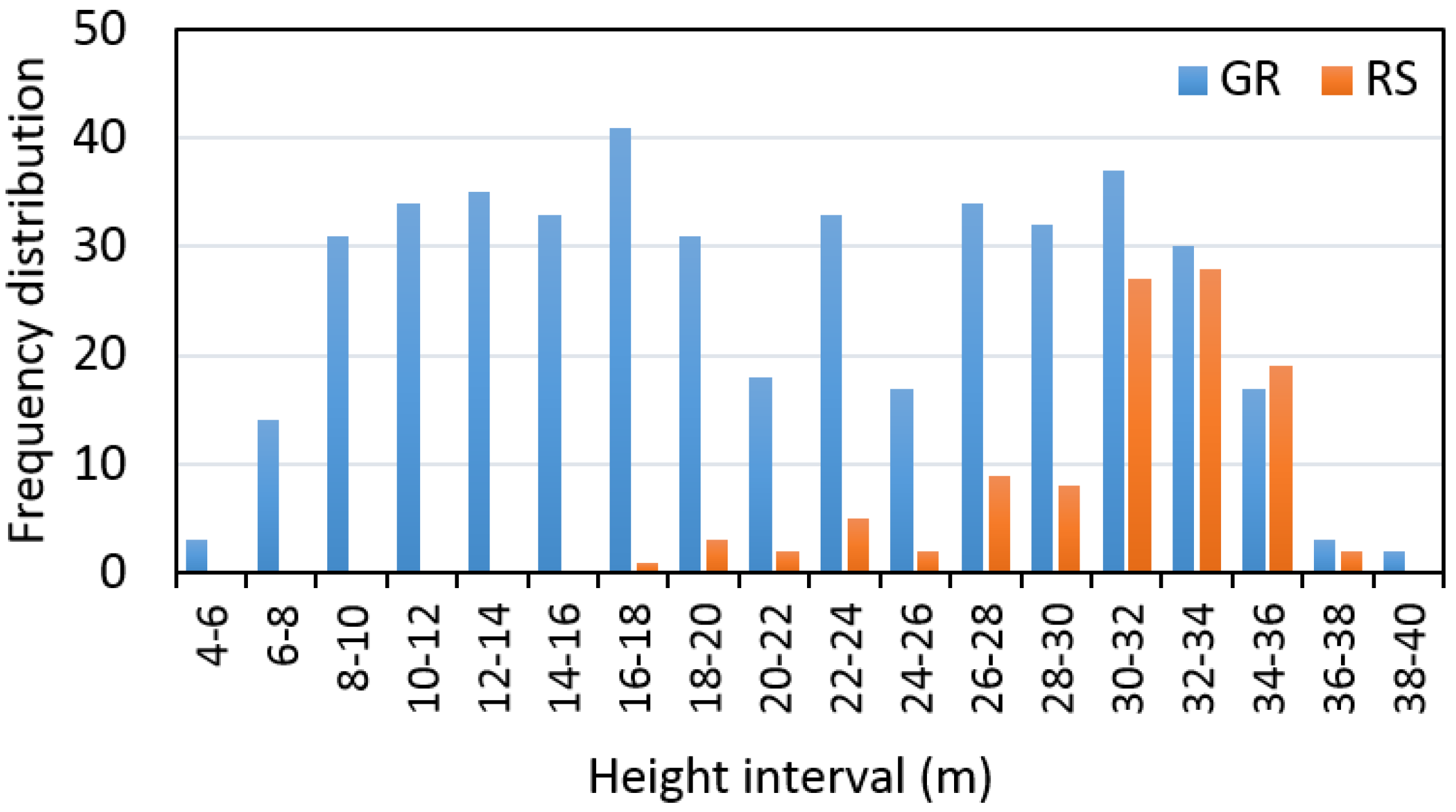
3.2. Accuracy of Tree Height Evaluation
The distribution of trees measured on the ground and remotely-sensed trees within the 2-m height intervals are presented in
Figure 3.
The results of the accuracy assessment for the evaluation of tree and stand height, based on airborne LiDAR data, are shown in
Table 3.
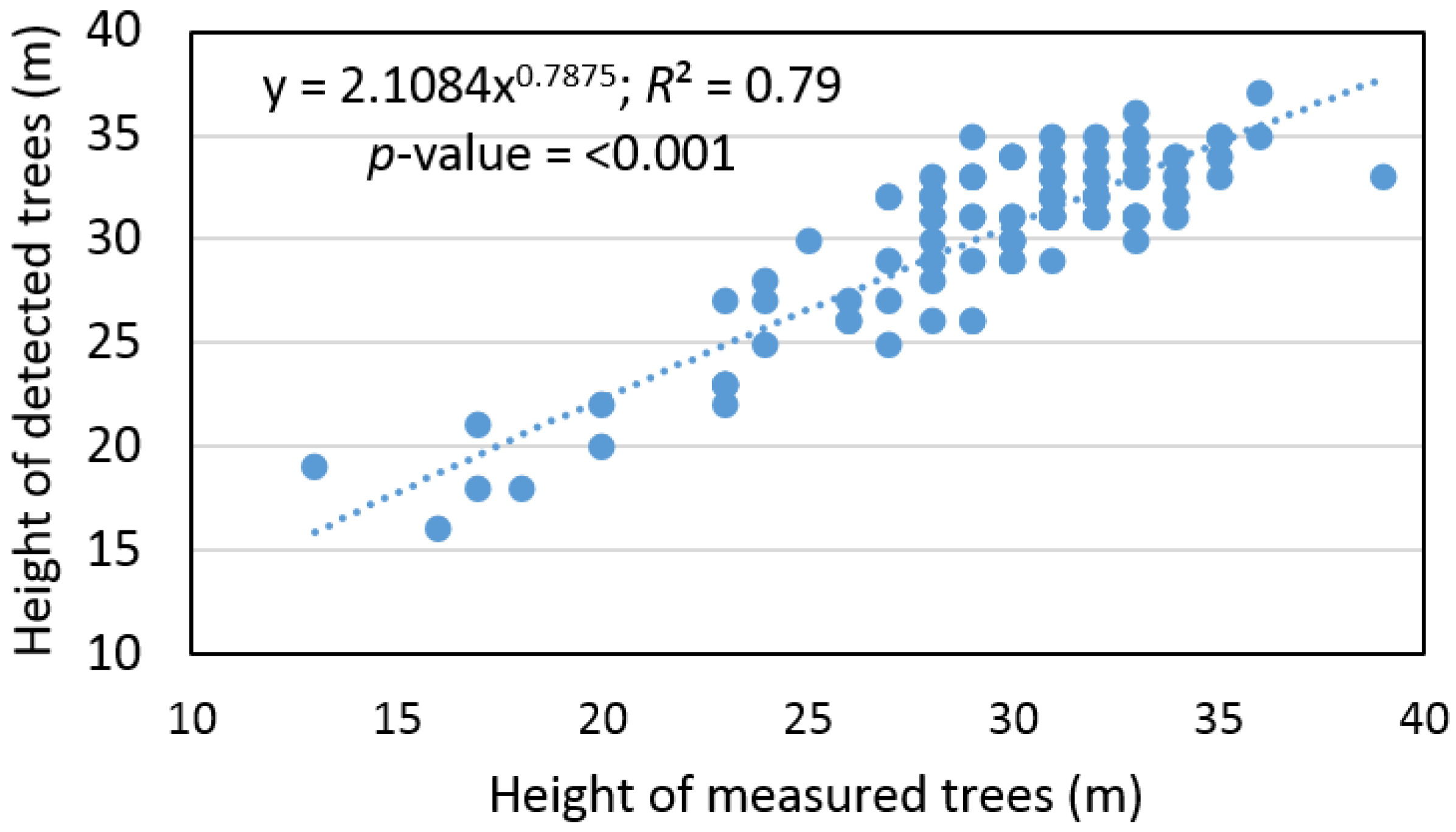
Based on the sample size, which contains pairs of measured and detected trees, the remote-based approach overestimated tree height by 3% ± 9%, and the RMSE% was ±8%. At the same time, we found that the tree height evaluated, based on ALS data, provided an output with differences that were statistically significant relative to the ground data (
α = 0.05). On other hand, we found a significant relationship (
R2 = 0.79) between the height of measured and detected trees (
Figure 4).
While the stand height, calculated based on remotely detected trees, reached a value of 30.3 m, the stand heights calculated based on measured trees were 25.9 m, 32.1 m, and 31.6 m, for mean height, mean height of 10% trees with the largest diameters, and mean height of 20% trees with the largest diameters, respectively.
3.3. Accuracy of Tree Diameter Derivation
General information of all significant regression models for predicting tree diameter from tree height is presented per tree species in
Table 4. We found that the derived tree diameter using the regression model was systematically underestimated in the case of dominant trees and systematically overestimated in the cases of trees from other social positions (
α = 0.05). Therefore, all results of derivation were corrected with respect to a bias value for dominant, codominant, intermediate, and suppressed tress.
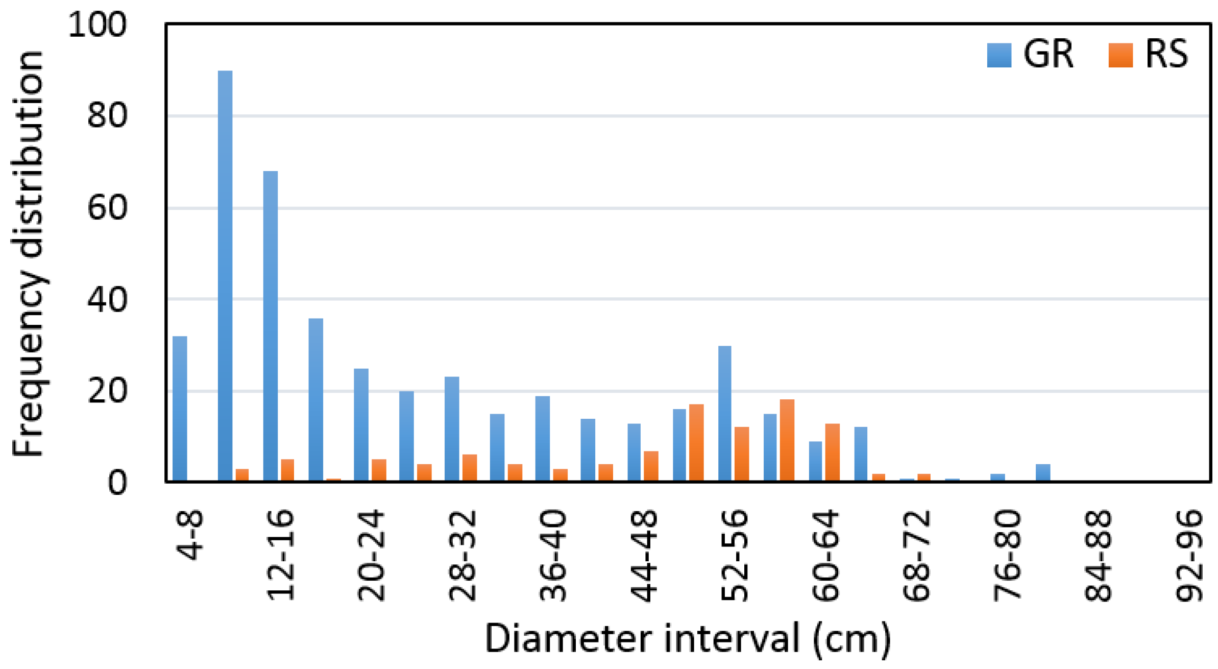
The distribution of trees measured on the ground and remotely-sensed trees within the 4-cm diameter interval are presented in
Figure 5.
The results of the accuracy assessment for tree and stand diameter derivation, based on airborne LiDAR data, are shown in
Table 5.
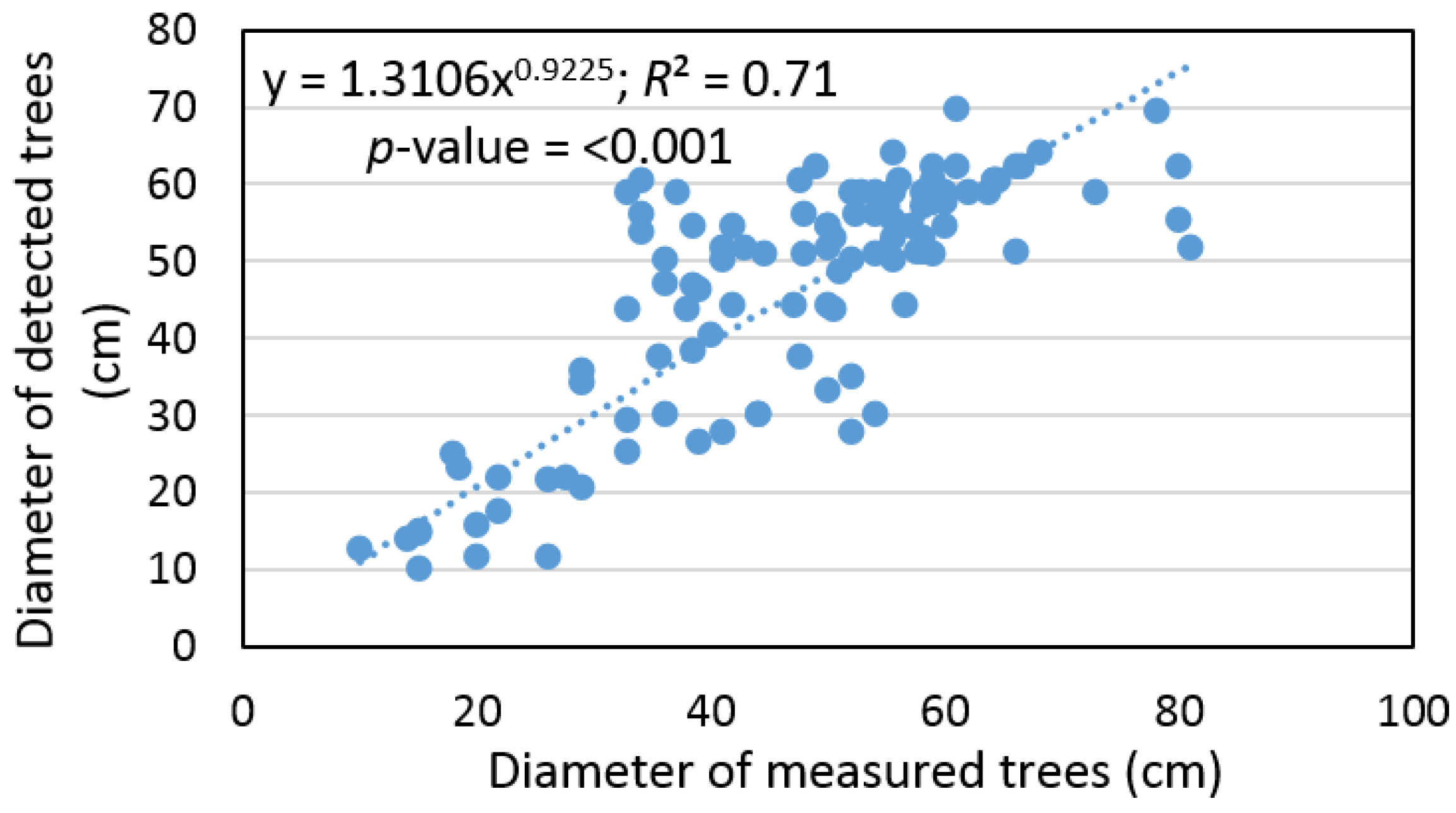
Based on the sample size, which contains pairs of measured and detected trees, the remote-based approach was corrected using a bias value that underestimated tree diameter by 1% ± 25% and the RMSE% was ±22%. At the same time, we found that tree diameter, detected based on ALS data, provided an output with a difference that was not statistically significant relative to the ground data (
α = 0.05). In addition, we found a significant relationship (
R2 = 0.71) between the diameter of measured and detected trees (
Figure 6).
While stand diameter calculated based on remotely-sensed trees reached a value of 46.1 cm, the stand diameters calculated based on measured trees were 32.9 cm, 63.7 cm, and 58.7 cm, for the mean diameter of all trees, mean diameter of 10% of trees with the largest diameters, and mean diameter of 20% of trees with the largest diameters, respectively.
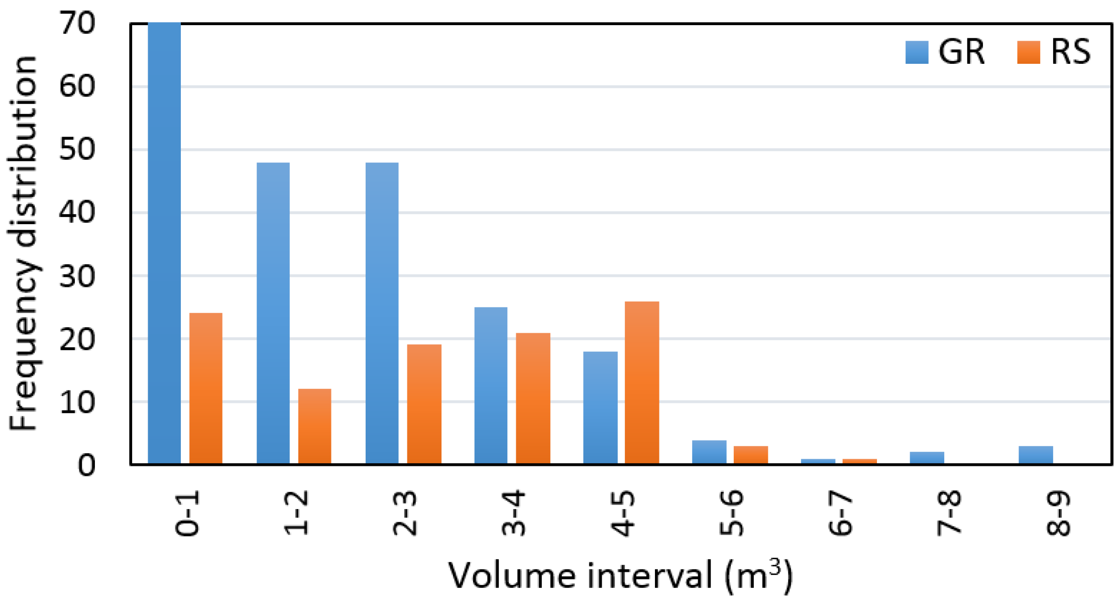
3.4. Accuracy of Tree Volume Calculation
As was the case for the tree diameter derivation, the results of volume calculation were under- or overestimated. However, the bias value was not significant and, therefore, the results of calculation were not corrected.
Distribution of trees measured on the ground and remotely-sensed trees within the 1-m
3 volume interval are presented in
Figure 7.
The results of the accuracy assessment for tree and stand volume calculation, based on airborne LiDAR data, are shown in
Table 6.
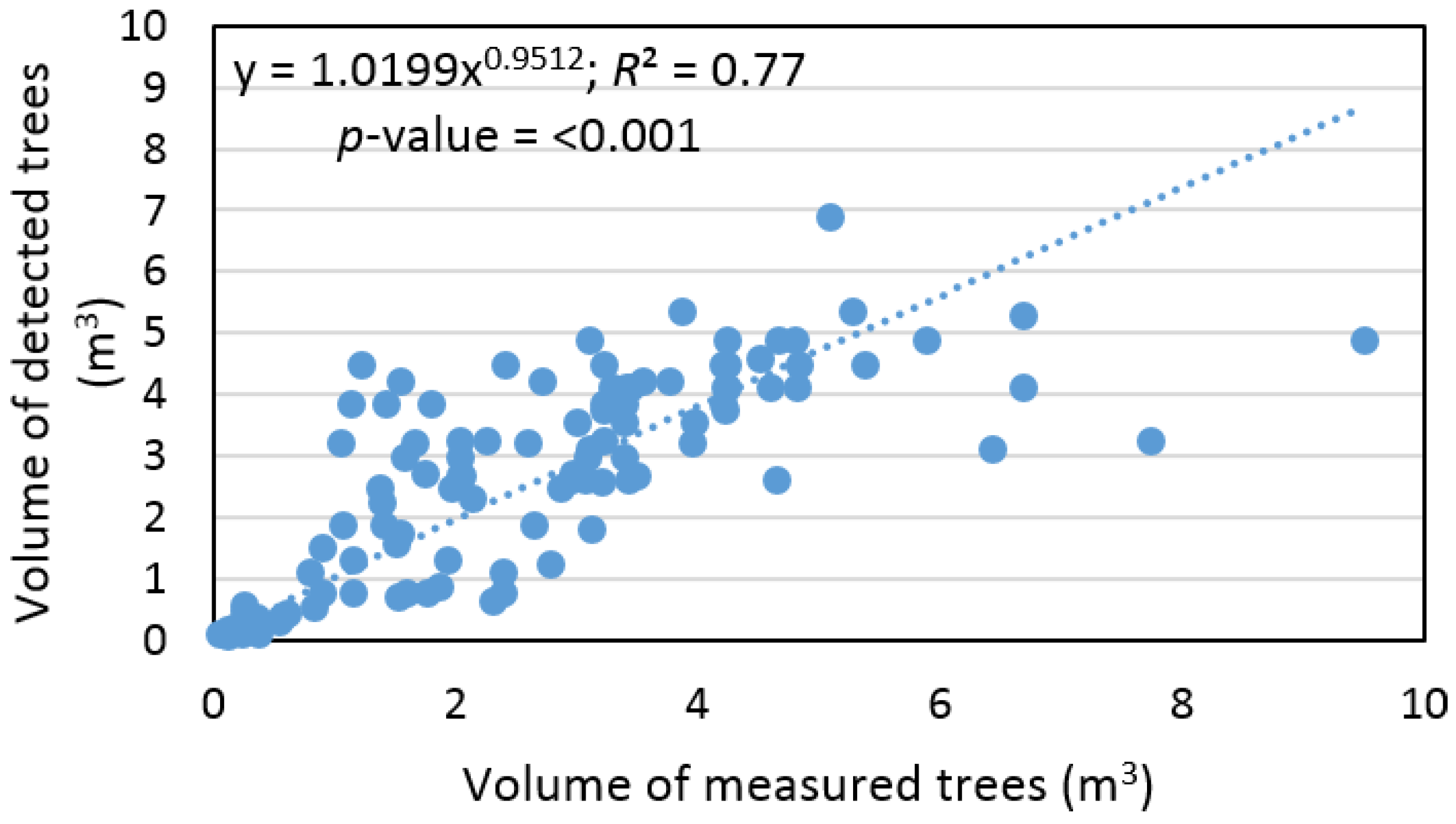
Based on sample size, which contains pairs of measured and detected trees, the remote-based approach overestimated tree volume by 1% ± 61% and the RMSE% was ±46%. At the same time, we found that tree volume, calculated based on ALS data, provided an output with a difference that was not statistically significant relative to ground data (
α = 0.05). In addition, we found a significant relationship (
R2 = 0.77) between volume of measured and detected trees (
Figure 8).
While the stand volume calculated based on remotely-sensed trees reached a value of 289.7 m3, the stand volume calculated based on measured trees was 507.0 m3. The total growing stock differed by −43% from the ground reference data, and detection rate was 64% for dominant, 58% for codominant, 36% for intermediate, and 16% for suppressed trees.
4. Discussion
In this study, we explored the opportunities using lightweight aerial scanner for the estimation of main forestry variables with a single-tree detection algorithm over a selected type of multilayered deciduous forest. In the following sections, we discuss the findings, compare our results with other studies, and outline methods to improve performance. Archived results, however, could be different under other conditions, where there may be other forest types or data sources. It should be also noted that measurement errors, related to the accuracy of measurement equipment, play an important role in presented results.
4.1. Single-Tree Detection
Our findings indicated that the single-tree detection algorithm, with optimal settings for local conditions, can capture approximately 66% dominant, 48% codominant, 18% intermediate, and 5% suppressed trees. False positive detection (commission rate) was relatively low, and ranged between 4% and 9%.
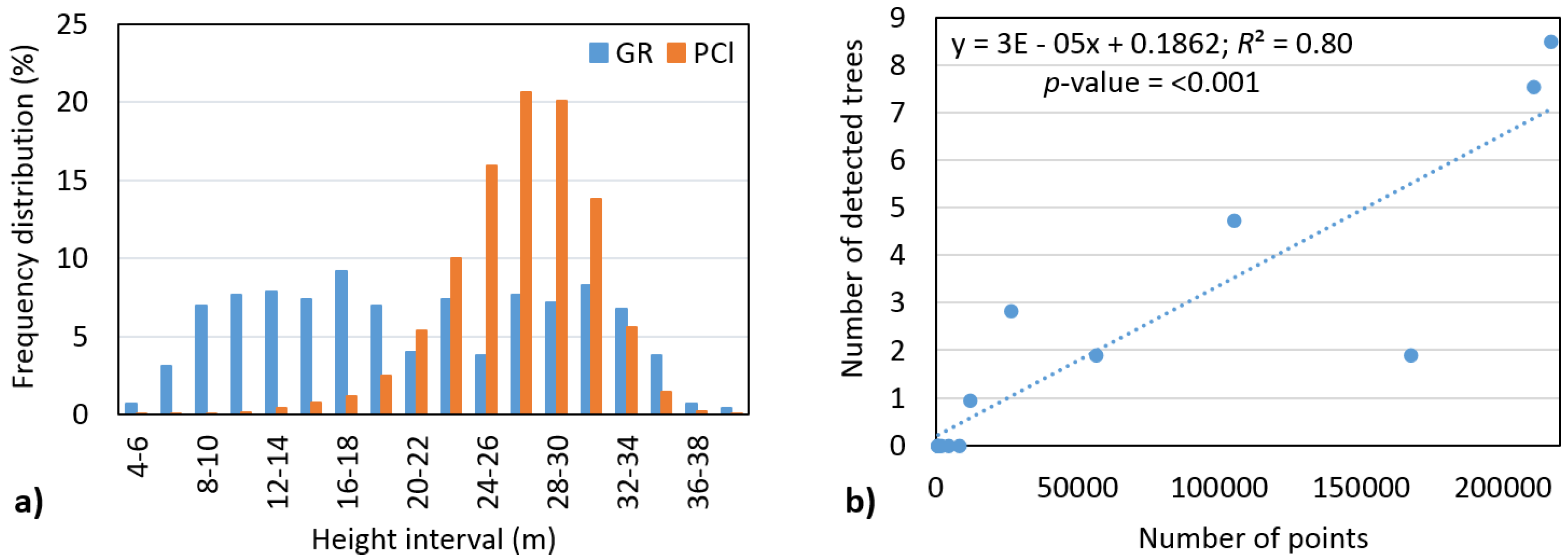
There are several factors that could have affected the accuracy of tree number detection in our assessment, which should be considered when interpreting our findings. First, clearly, the individual tree detection algorithm is best suited to finding dominant trees; however, the ground reference data include only 12% dominant and 22% codominant trees. Second, most of the points in the point cloud are related to height ranges of 16–36 m (95% of points) and 21–31 m (68% of points), respectively (
Figure 9a). For example, only 5% from all points is situated in the 2–20 m space, but it accounts for 59% of trees. This means that, based on objective reasons, identification of these trees is very difficult. Therefore, we then investigated the effect of number of points on number of detected trees in the height range of 2–20 m. We found a significant relationship (
α = 0.05) with a strong correlation (
R2 = 0.80) (
Figure 9b). Thus, having more points from intermediate echoes causes a significant increase in the detection rate of trees below the main canopy layer.
In similar conditions, such a detection rate has also been reported by other authors, and relates to the crown morphology of deciduous species with indistinct treetops. Furthermore, a dense crown canopy also causes most of the points from a LiDAR point cloud to be concentrated within the main canopy layer. Therefore, detection of understory trees is difficult. International research has suggested that detection rates fluctuated around 50%, and RMSE% varied from 45% to 89% (e.g., [
38,
39,
40,
41]). On the other hand, the commission error of our own method did exceed the accuracy reported by other research. For example, within the single tree detection benchmark inside the NEWFOR project [
42], the commission rate varied from 7% to 141%. Thus, the geo-dendrometric criteria included in the presented algorithm has been successful in suppressing most false treetops, such as protruding branches, multiple terminals, and other morphological patterns that can be present in tree crowns.
With respect to the density of the 30 hits per square meter used in this study, we do not assume that an increase in scanning density could improve the accuracy of detection of dominant and codominant trees. However, the combination of ALS data, from the leaf-on and leaf-off seasons, may be appropriate for increases the chance that more points could penetrate the canopy, and that the detection rate of trees growing under the canopy could increase with a higher scanning density.
4.2. Tree Height Evaluation
Related to the individual tree height, ALS data generally provide remote-based measurements that are highly correlated with field-based measurements. Although the precision of field measurements of tree height in deciduous forests with a dense canopy layer is limited, which influences total accuracy, we confirmed the relationship by a strong correlation with an R2 value of 0.8. We also found that the tree height evaluated by the algorithm was systematically overestimated relative to the testing data, and total accuracy in terms of RMSE reached 2.4 m (8%). In the case of stand height, the differences between measured and evaluated values were in the range of −1.8 m (−6%)–4.5 m (17%), for top and mean height, respectively. The mean height, evaluated based on ALS data, was most similar to the mean height of 20% of measured trees with the largest diameter.
A similar approach for tree height evaluation to that in our study was used by Brandtberg et al. [
43] and Gaveau and Hill [
44], where evaluated LiDAR tree heights acquired in leaf-off conditions over a deciduous forest reached an overall standard error of 1.1 m, or canopy surface height was underestimated by 0.91 m in shrub canopies, and 1.27 in tree canopies. Chávez and Tullis [
45] evaluated tree height using ALS data and a spectral predictor over full-canopy oak-hickory forests with an average error of 1.67–2.99 m, RMSE of 2.2 m, and the correlation coefficient ranged between 0.42 and 0.51.
4.3. Tree Diameter Derivation
Although our model for tree diameter derivation is relatively simple (one-parameter nonlinear function), and not as accurate as those used by other studies that specialize on this topic (e.g., [
46,
47]) regression between pairs of identical detected and measured trees is encouraging (
R2 = 0.71). After bias correction, the overall accuracy reached 10.2 cm (22%). In the case of stand diameter, the differences between measured and derived values were in the range of −17.6 cm (−28%) to 13.2 cm (40%) for top and mean diameter, respectively. The mean diameter, evaluated based on ALS data, was most similar to mean diameter of 20% of measured trees with the largest diameters.
Several authors [
48,
49] have provided extensive research on predicting stem diameter using ALS data in a temperate forest. The proposed regression models included multilinear regression, least square boosting decision trees, random forest, and ε-support vector regression. As LiDAR metrics were used, variables, such as tree height, crown area, crown height, and crown volume, were extracted based on the ITD approach. These studies achieved accuracies of 15%–23%, in terms of RMSE%.
4.4. Tree Volume Calculation
Our findings indicated that the presented approach captured approximately 57% of the stand volume in the study area. The calculated volume was distributed as 64%, 58%, 36%, and 16%, for dominant, codominant, intermediate, and suppressed trees, respectively. No significant differences were found between stem volumes of pairs of measured and detected trees. Therefore, volume calculation was executed without statistical correction, and we found a RMSE% of 1.2 m3 (46%) and a correlation with an R2 value of 0.8.
While the presented ITD approach for volume calculation is based on tree height and diameter, several studies also used a combination of tree and stand variables. For example, Naesset [
50], in a mature forest area, used a percentile of pulse laser heights and canopy density, with an
R2 that ranged from 0.83 to 0.86. The approach by Tesfamichael et al. [
51] combined a LiDAR-derived height variables, stems per hectare, as well as stand age, and the level of association between estimated and observed volume in eucalyptus plantations was relatively high (
R2 = 0.82–0.94) with negative biases and a RMSE ranging in the order of 20%–43%. Many authors have also reported methods for volume estimation, based on the ABA approach. In these cases, the biophysical forest variables are regressed against ALS metrics, and such a statistical relationship can be approximated by, for example, linear models [
52], non-parametric approaches, including nearest neighbors imputation [
53], linear mixed effects models with random stand-level intercepts [
54], or Bayesian methods [
55].
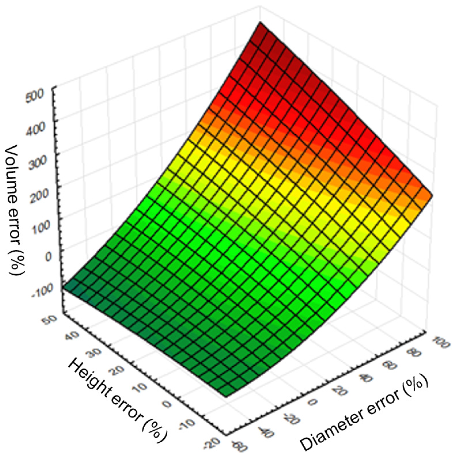
Accuracy of assessment of tree and stand volume using the ITD approach ultimately depends on the accuracy of the underlying characteristics, and is affected by the accumulation of errors from single tree detection, tree height evaluation, tree species classification, and diameter derivation [
56,
57,
58]. In our study, we confirmed multiple significant and strong relationships (
R2 = 0.96) between relative mean errors of remote-based volume, tree height, and tree diameter (
Figure 10). In general, a method for increasing the accuracy of stem volume calculation lies in improving the methods of detection, feature extraction, and estimation for each underlying characteristic.
5. Conclusions
The main objective of this study was to assess the usability and accuracy of our own single-tree detection algorithm within a remote-based forest inventory, using LiDAR data from lightweight aerial scanner for a selected type of multilayered deciduous forest.
Results show that this approach can be used for detecting single trees and measuring (or derivation of) various biophysical tree variables, such as height, diameter, and volume. With respect to other studies, our findings also indicated that airborne LiDAR data are suitable, mainly for the evaluation of tree height. The algorithm has less success for tree detection, tree diameter derivation, and volume calculation. In this context, the detection rate of understory trees typically depends on point density across a point cloud, and the accuracy of stem diameter derivation depends on the model used. Finally, it is important to note that the results of accuracy assessment depend on the accuracy of reference data as well.
Therefore, future research should be concerned with building more precise models for stem diameter derivation and developing algorithms for tree-species classification. Future research should also be carried out to apply the presented approach within a praxis of forest inventories under different ecosystems and data quality.


