Estimation of Tree Stem Attributes Using Terrestrial Photogrammetry with a Camera Rig

Abstract

We propose a novel photogrammetric method for field plot inventory, designed for simplicity and time efficiency on-site. A prototype multi-camera rig was used to acquire images from field plot centers in multiple directions. The acquisition time on-site was less than two minutes. From each view, a point cloud was generated using a novel, rig-based matching of detected SIFT keypoints. Stems were detected in the merged point cloud, and their positions and diameters were estimated. The method was evaluated on 25 hemi-boreal forest plots of a 10-m radius. Due to difficult lighting conditions and faulty hardware, imagery from only six field plots was processed. The method performed best on three plots with clearly visible stems with a 76% detection rate and 0% commission. Diameters could be estimated for 40% of the stems with an RMSE of 2.8–9.5 cm. The results are comparable to other camera-based methods evaluated in a similar manner. The results are inferior to TLS-based methods. However, our method is easily extended to multiple station image schemas, something that could significantly improve the results while retaining low commission errors and time on-site. Furthermore, with smaller hardware, we believe this could be a useful technique for measuring stem attributes in the forest.

1. Introduction

Forest owners, governments and environmental organizations need forest information for economic, planning and preservation purposes. Biomass, wood volume and carbon storage are some of the used variables. The diameter at breast height (DBH) is the single most important parameter for the estimation of forest information. DBH is usually measured manually with a caliper or a measuring tape and is recorded together with species during field inventories [1]. The individual tree positions can be determined using a total station or ultrasonic trilateration. The positions are useful for the training of remote sensing methods at the single tree level [2,3], but the acquisition cost is high [4]. As the current manual inventory methods used to collect forest information are resource intensive, there is a demand to find less expensive methods.

Many methods for simplifying DBH measurement using non-contact methods have been proposed over the last 100 years, summarized by Clark et al. [5]. They found that accuracy, productivity and cost requirements, as well as practical restrictions must be considered to evaluate if a project benefits from a new instrument compared to traditional field measurements.

During the last two decades, the rapid development of laser scanners and digital cameras has made three-dimensional (3D) point clouds a useful data source for tree measurements. Terrestrial laser scanner (TLS) methods generate dense point clouds of the scene visible from the scanner. Tree detection methods have been developed that detect trees in the point clouds resulting from either a single scan [6,7], co-registration of multiple scans [8,9] or from scans obtained by personal laser scanning (PLS) with portable units [10].

Compared to TLS methods, camera-based methods offer potentially less expensive hardware, increased mobility and reduced time on-site. Early attempts at photogrammetric measurements based on analog images were however abandoned due to excessive manual processing times [11].

Most recent methods have been based on the use of a single digital camera, either handheld or mounted on a UAV [12,13,14,15,16]. Although several single-camera reconstruction results are impressive, all methods except [15] were evaluated in park-like conditions, i.e., on effectively free-standing trees viewed from multiple directions in reasonably good lighting conditions. Those methods would be difficult to apply to the occlusion-rich environment of a forest. The method of Liang et al. [15] is, to our knowledge, the only published method that has been evaluated in a forest. As published, the method is quite time consuming on site, where a large number of images and some supporting manual measurements need to be acquired. Another paper by Rodríguez-García et al. [17] presents a method that used purpose-built stereoscopic hardware and was evaluated on a plantation plot.

In this paper, we present a novel method to measure DBH and tree positions on field plots using a calibrated multi-camera rig. The calibration information is used to improve the quality of the produced point cloud by reducing the number of false matches. Furthermore, the point cloud is automatically scaled without any additional measurements or targets in the scene.

The aim is to create a method that is robust and simple to use in a forest environment, faster than manual inventory and that uses less expensive and more commonly available equipment than TLS. The emphasis has been on simplicity and low time requirements on-site. The objectives were to (1) develop a method using a multi-camera rig that produces estimates of DBH and tree positions on plots and (2) evaluate the method on multiple forest field plots in terms of the level of tree detection, the time requirement and the error and bias of the DBH measurements.

2. Materials and Methods

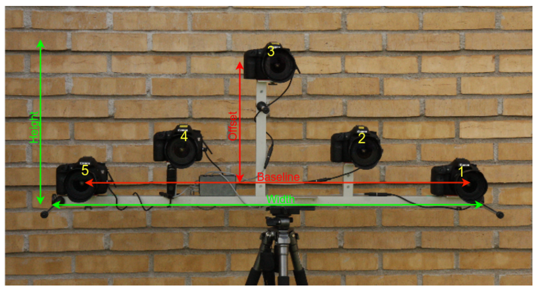
2.1. Rig and Image Protocol Design

A prototype camera rig was designed with two main requirements in mind: simplicity on-site and redundancy. The choice of a camera rig is based on the simplicity criteria; a rig gives a point cloud from only one exposure, which simplifies the image acquisition protocol, and the scale of the point cloud will be known from the rig baseline. The redundancy requirement stemmed from the expectation that the imaging would be performed in an occlusion-rich environment where the tree trunks could be partially obscured by, e.g., tree branches, undergrowth and other tree trunks. Furthermore, the data analysis should favor high quality over high density, i.e., a low density point cloud with few outliers was considered more important than a high density point cloud with many outliers. As two-camera matches have the potential to generate a large number of outliers, matches between a minimum of three non-collinear cameras were to be required in order to produce a 3D point. Any calibrated rig removes the need for a scale bar, since the known length of the rig baseline establishes the scale of the scene. To satisfy the other requirements, the rig was designed with five cameras in positions such that no three-camera subset was collinear ([18] and Figure 1). The five-camera design would be tolerant towards occlusions, since matching between any combination of three cameras would be sufficient to produce a point. The rig was chosen to be as wide as possible to maximize occlusion tolerance and still be able to be transported by a standard road car. As the resulting optical baselines of the different camera triplets varied between 57 and 113 cm, accurate measurements would be possible for ranges between 1 and 20 m.

The chosen image acquisition protocol was the simplest possible: take all images from the center of the field plot, looking outwards in different directions. The separation between view directions was set to 30 degrees, expected to be well within the overlap of the “left-looking” Cameras 1–2–3 and “right-looking” Cameras 3–4–5 in subsequent view directions, respectively. A standard magnetic compass was mounted on the rig as an alignment guide.

Three new Canon EOS 7D cameras with Sigma EX20/1.8 DG fixed lenses were attached to the rig at Positions 1, 3 and 5. Furthermore, two Canon EOS 40D cameras equipped with Canon EF–S 17–55/2.8 zoom lenses from a previous project were attached at Positions 2 and 4. The zoom rings were fixed with duct tape to minimize movement. The nominal focal lengths were 20 mm (Sigma) and 17 mm (Canon), respectively. All auto-focus and image stabilizing features were turned off. The cameras were synchronized by a cable trigger. Unfortunately, both 40D cameras were later found to have insufficient optical stability (see Section 2.4) and were only partially used in the study.

The total weight of the rig was about 13 kg. EasyRig 2.5 [19], a support system for TV cameras, was used to carry the rig in the field (Figure 2). A similarly equipped rig would, with hardware available in 2016, cost about 7000 EUR (3 cameras) to 10,000 EUR (5 cameras), including cameras, lenses, EasyRig 2.5 and construction of the rig. An example of images from Cameras 1, 3 and 5 is shown in Figure 3.

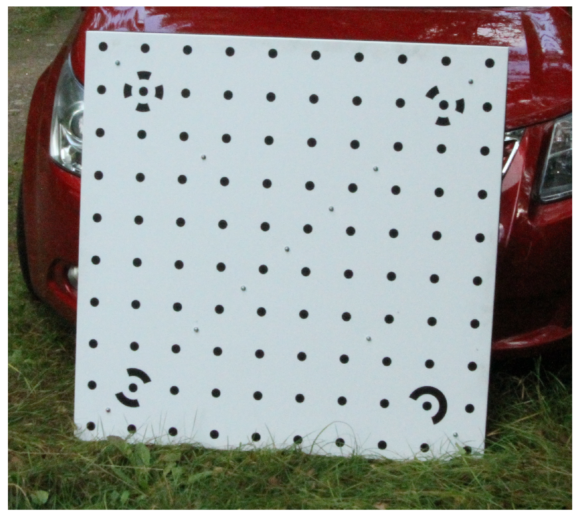
2.2. Calibration

The calibration protocol specifies that each camera is individually calibrated at the beginning and end of a field campaign. About 25 images of a 1 m square planar calibration target (Figure 4) were acquired by each camera from different angles and distances. The calibration markers were measured semi-automatically and processed by the algorithm of Börlin and Grussenmeyer [20]. The calibration process was repeated at the end of the campaign to assess the optical stability of each camera. The calibration process estimates the internal geometry of each camera, for example the focal length and lens distortion parameters, and is essential for the subsequent image processing. The exposure parameters were chosen as a compromise between a high depth of field and a small motion blur; infinity focus, maximum ISO (7D: 6400; 40D: 1600), aperture f/11 and variable exposure time. The exposure parameters, except exposure time, were kept fixed throughout the campaign.

The rig was calibrated before and after each field plot to make it possible to detect any disturbances. Two image sets of double exposures of the calibration target were taken at about a 4- and 8-m distance. The calibration targets were measured semi-automatically, and the relative orientation of the cameras in the rig was estimated using the damped bundle adjustment algorithm by Börlin and Grussenmeyer [21]. The center camera provided the reference point, and the positions and the directions of the other cameras were calculated in the reference point’s coordinate system. In total, four rig calibrations were computed using the before/after rig calibration images and the beginning/end camera calibration images. The calibration with the smallest residual was used in the processing of the plot images.

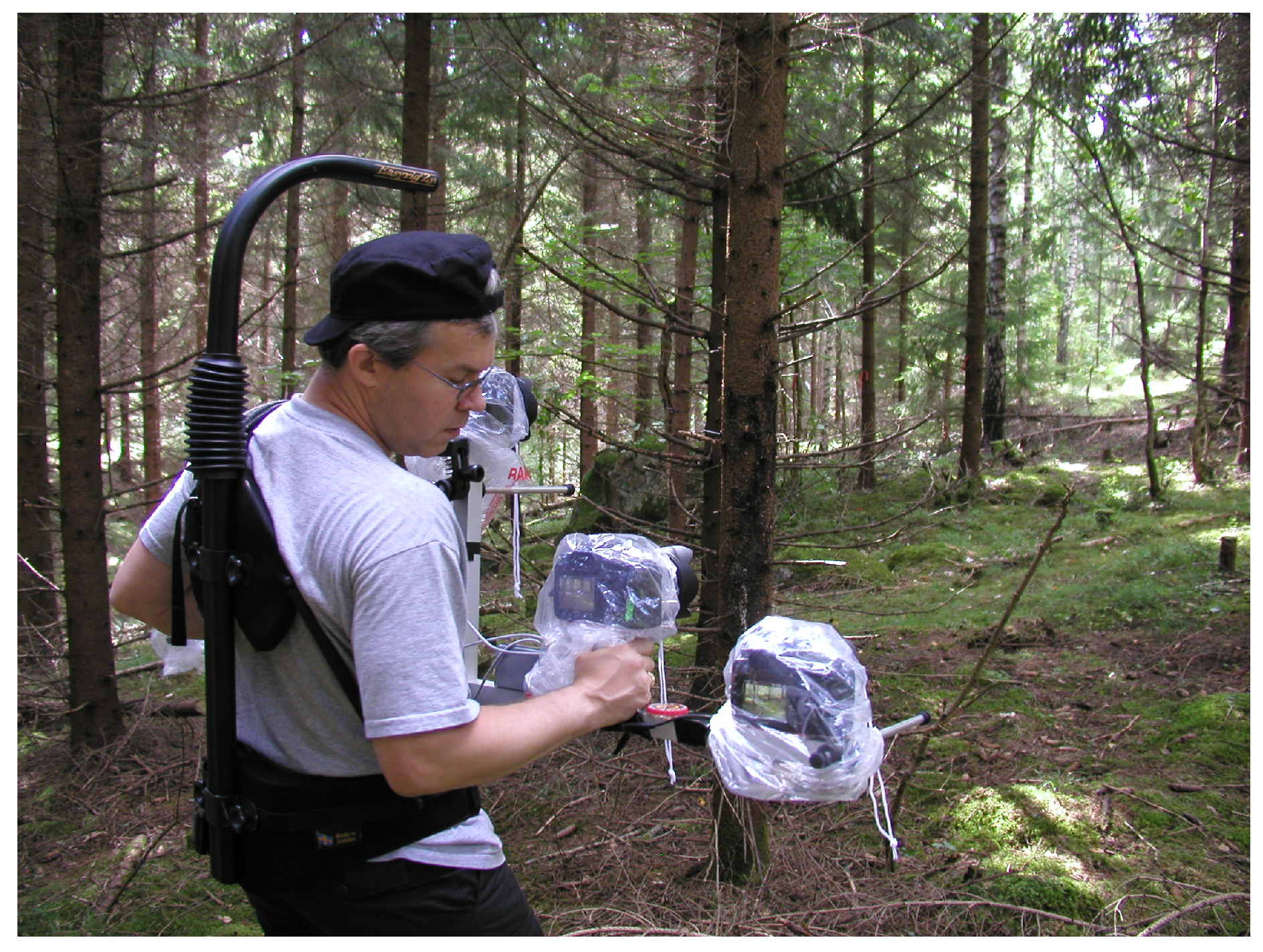
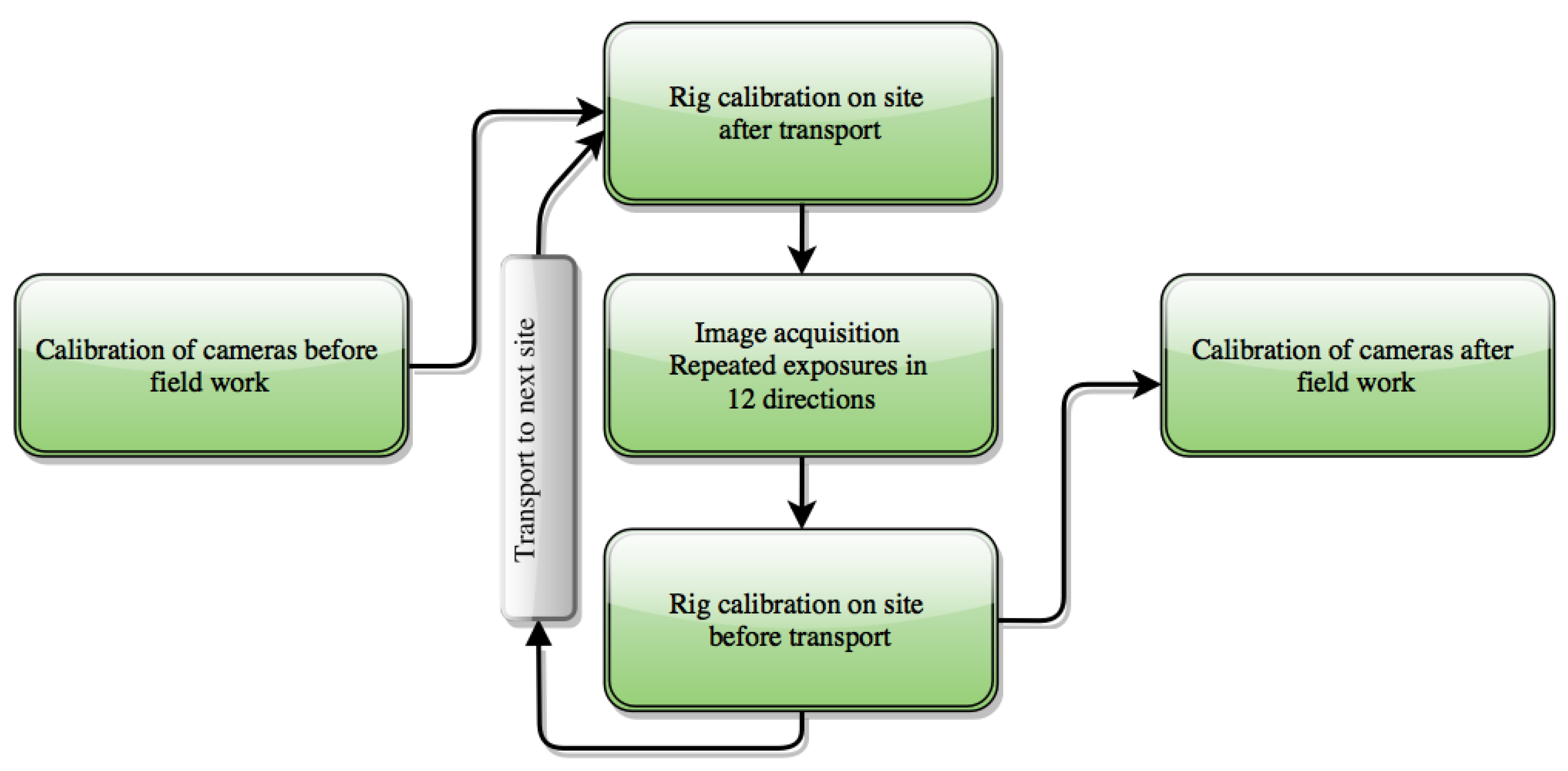
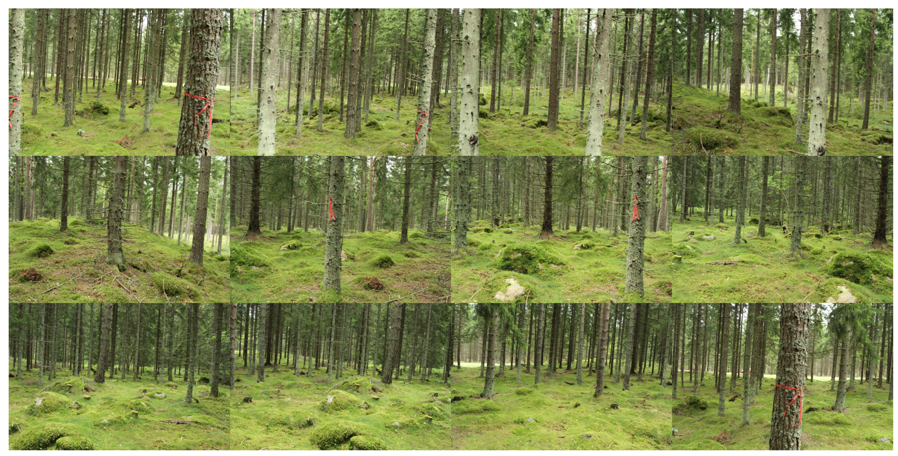
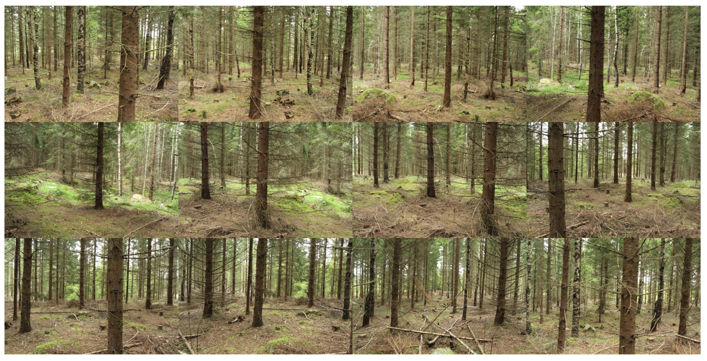
2.3. Field Work

A dataset was acquired during a three-day field campaign at the Remningstorp estate (N58.46°, E13.65°) in southern Sweden. The forest is hemi-boreal and dominated by Norway spruce and Scots pine with some deciduous trees, mostly birch. Images were collected on 25 field plots with a 20-m radius. The plots were selected to include various forest types, ages, species composition and stem density. Ground truth data were gathered for each field plot. The DBH of each tree was measured crosswise with a caliper. Tree positions were acquired using a total station.

The rig was transported by car to a location within 1 km of each plot. After off-loading, the rig was carried through the forest using the EasyRig harness. Before and after each forest excursion, images of the calibration target were taken by the rig as described in Section 2.2 (For simplicity, the word image(s) is sometimes used to indicate a set(s) of images, simultaneously acquired by the rig cameras when the distinction is unnecessary or clear from the context. For the same reason, repeated exposures to prevent data loss are sometimes not mentioned). On the plot, images were acquired from the approximate plot center in 12 directions, separated by approximately 30 degrees. The magnetic compass was used as an aiming guide. To guard against data loss due to bad connectors, each exposure was repeated, both on-plot and for the rig calibration images. The flowchart in Figure 5 shows a visualization of the workflow.

Approximately 15–25 min were spent for data acquisition per site. This includes time for loading and unloading the equipment from the car, rig calibration image acquisition at the car and walking between the road and the field plot. Less than two minutes were spent to acquire the images on the field plot.

2.4. Reduction of the Dataset

The re-calibration of the cameras after the campaign revealed that Camera 4 was optically unstable. Similarly, the stability of Camera 2 was questionable. For this reason, no images from Camera 2 nor 4 were used for the point cloud construction. The Camera 2 images were still used to aid co-registration; see Section 2.5. The near limit for the reduced 1–3–5-camera rig, i.e., the shortest distance in front of the rig where a 3D point is simultaneously visible in all cameras, was about 1 m.

Of the 25 field plots, one plot was discarded due to a disturbance of the rig during the image acquisition. Furthermore, about twelve of the plots posed challenges due to hard light, that made the stems too dark for feature detection in some directions. As the system requires a 360-degree view, if images from one direction were unusable, the whole plot had to be discarded. Of the remaining field plots, six plots were eventually processed, numbered 32, 87, 165, 167, 203 and 343 with tree density and DBH as presented in

Table 1. Statistics for the processed plots. Diameter measurements in cm.

Plot	Trees	Trees/m${}^2$	mean DBH	min DBH	max DBH
32	29	0.09	23.1	11.9	35.7
87	38	0.12	22.8	5.0	35.7
165	25	0.08	24.1	10.5	34.5
167	22	0.07	19.2	5.2	30.8
203	34	0.11	21.0	3.8	37.0
343	12	0.04	19.3	7.1	29.9

.

2.5. Data Processing

We have implemented a data processing pipeline that requires a low level of operator interaction. The input data to the pipeline consist of images from one field plot and calibration images. From the images, a point cloud was calculated for each view and co-registered into a point cloud for the whole plot. The point cloud was segmented, and stems were detected. From the stem segments, the DBH was estimated by circle fitting to a 2D projection of the points closest to breast height (130 cm). An overview of the data processing pipeline is presented in Figure 6. A more detailed description follows in this section. As indicated in Section 2.4, only Cameras 1–3–5 were used to produce stem segments. A second point cloud using Cameras 1–2–3 was used in conjunction for the co-registration.

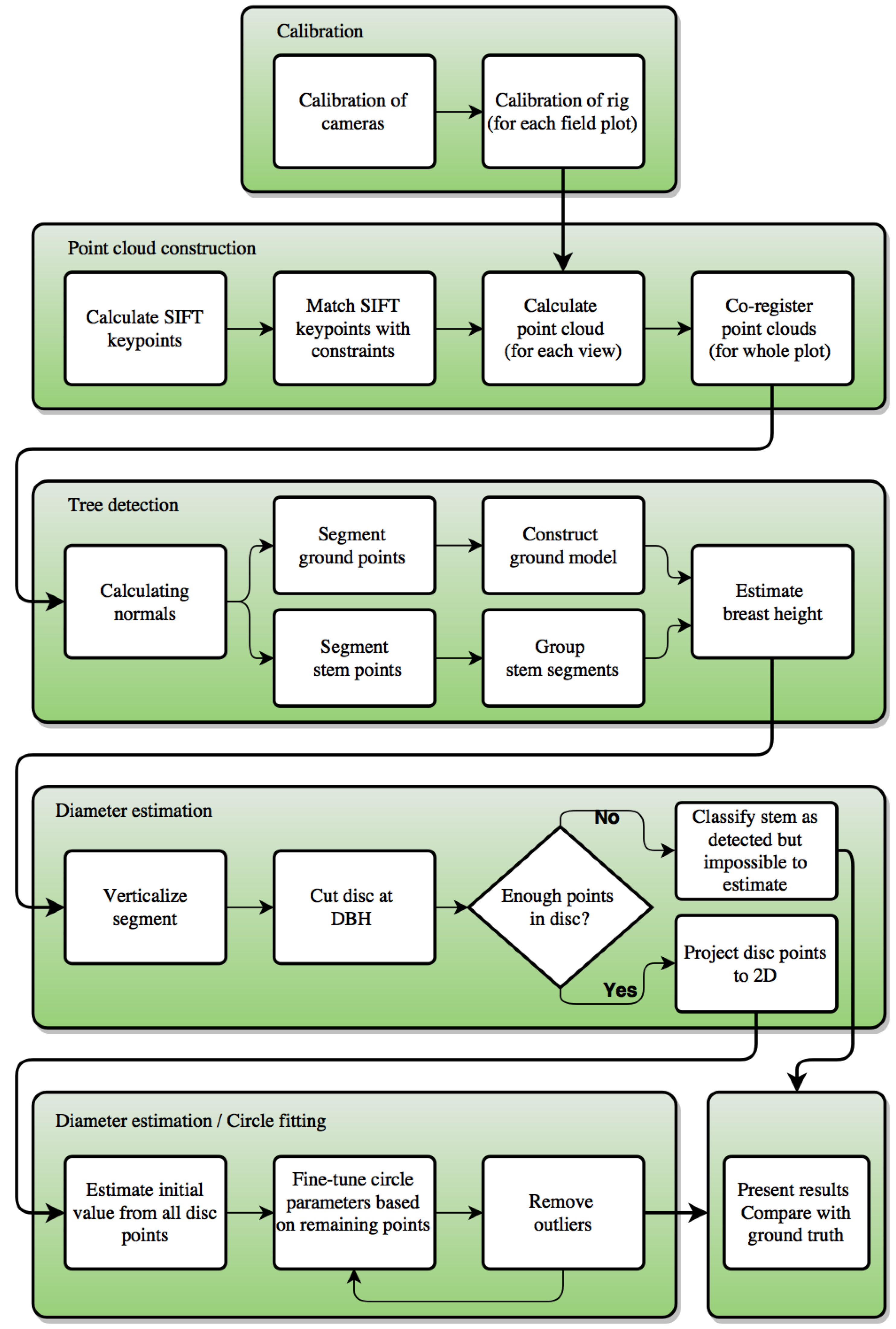
2.5.1. Calibration

The cameras and the camera rig were calibrated as described in Section 2.2. The rig calibration results were used for epipolar filtering of the matched keypoints and for calculation of the point cloud.

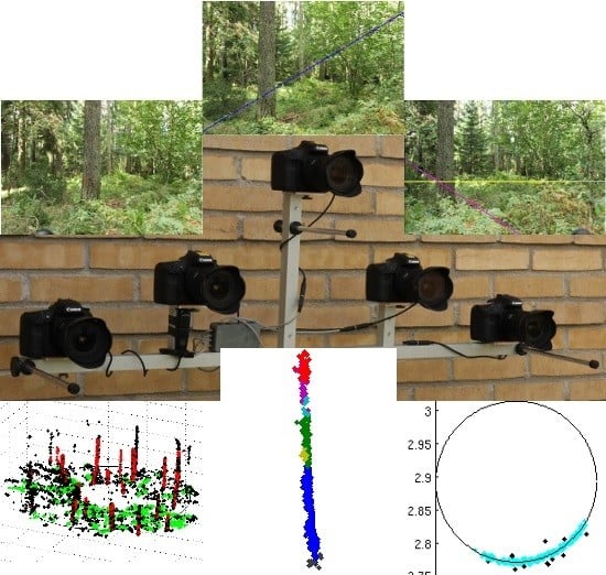
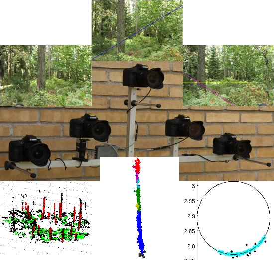
2.5.2. Point Cloud Construction

The algorithm for automatic point cloud computation was a development of the algorithm by Forsman et al. [18]. Each image was processed using the VLFeat (VisionLab Features Library) implementation of the Scale Invariant Feature Transform (SIFT) algorithm [22]. The SIFT algorithm detects keypoints that are characterized by four types of parameters: position, size, dominant direction and a descriptor. The descriptor describes the area near the keypoint and enables computation of the keypoint similarity independently of the other parameters. The SIFT keypoints detected in each image triplet were matched to generate a point cloud. Each point within the point cloud was generated from a three-way match between keypoints from each image. For a match to be accepted, the three keypoints had to satisfy the following criteria (matching thresholds are indicated in parenthesis):

• The keypoints should be similar, as judged by the normalized similarity ($\ge 0.75$) of the keypoint descriptors.
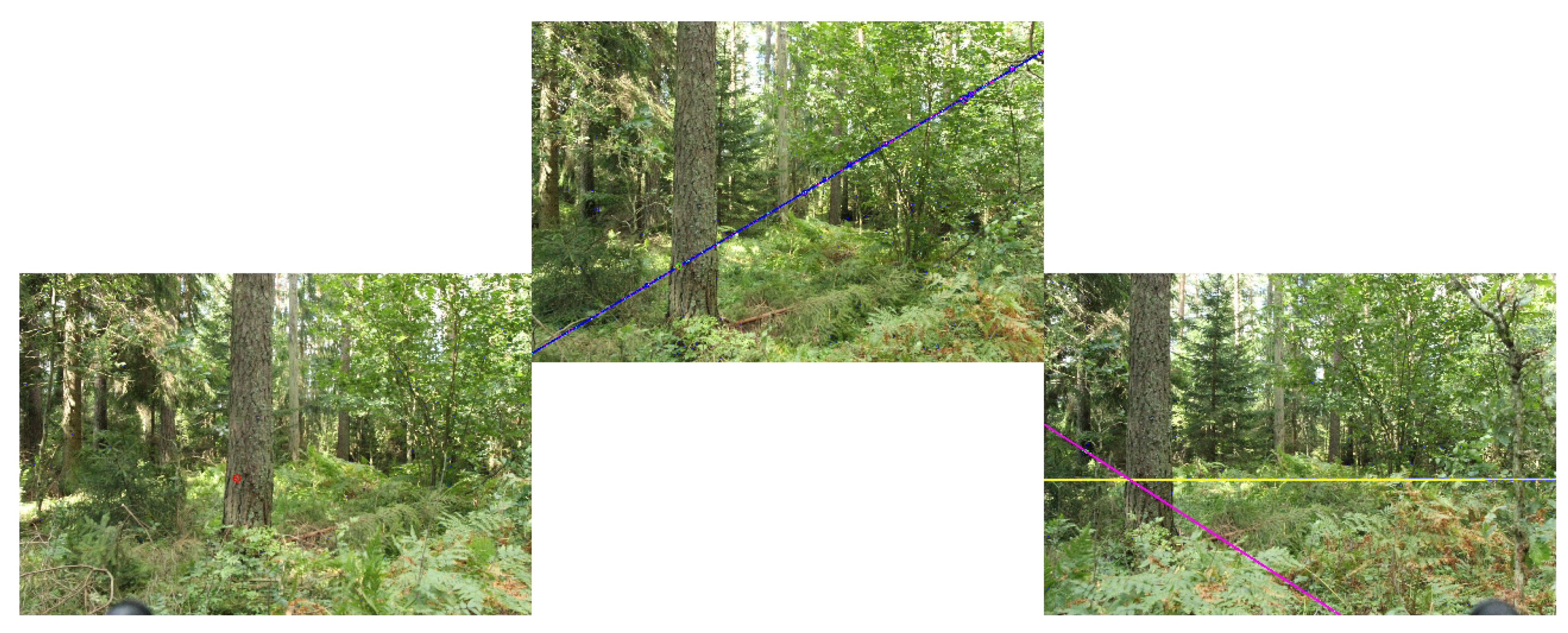
• The keypoints should correspond to the same 3D area, indicated by a similarity in keypoint size (within ±10%) and dominant direction (within ±30°). This requirement follows indirectly from the calibrated geometry of the rig, as an area at a distance of, e.g., 8 m should have roughly the same size and dominant orientation when viewed from the different cameras of the rig.
• The keypoints should correspond to the same 3D coordinate, as measured by the distance to the epipolar lines ($<5$ times the keypoint size) of the keypoints of the other images [23] (Chapter 9.1). This requirement follows directly from the calibrated geometry of the rig.

Given an accepted match, the 3D point position was computed from the positions of the three keypoints using spatial intersection [24] (Chapter 11.1.5). Figure 5 shows an image triplet with a keypoint and its corresponding epipolar lines.

The above process was applied to each view of the plot, generating 24 point clouds; two in each of the twelve directions. Each point cloud was computed in a local coordinate system with the rig center camera as the origin.

In order to merge all point clouds from one plot, the 24 point clouds needed to be co-registered. As the repeated exposures were not taken at exactly the same position, all point clouds were treated the same way. The co-registration was performed in two phases: a sequential phase and a global phase. In the sequential phase, common points between sequential views (1–2–…–24–1 ) were detected automatically using adaptive RANSAC on the rigid-body transformation [23,25] (p = 99.9%, s = 3). The RANSAC procedure was applied to all potential between-view matches of 3D points whose keypoints matched Criteria (A) and (C) above. The rigid-body transformations were computed by the SVD algorithm [26]. The consensus set-defining threshold for the transformation residual was 5 cm. In some cases, the automatic detection failed, because the point clouds from the different views had too few common points. The reason was often occlusions in one of the views that made the overlapping parts of the images differ too much. In these cases, some manual measurements were needed to augment the automatic points for the co-registration procedure to succeed. The estimated sequential rotations varied between 17 and 46 degrees.

In the absence of measurement errors, the sequential rigid-body transformations should form a closed loop, i.e., the concatenation of the 24 sequential rigid-body transformations should return to the original position of the rig in View 1. In practice, however, this did not occur. To correct for this deficiency, a global least squares adjustment procedure was applied to all points from the sequential phase using the Gauss–Helmert estimation model with the closed loop as a functional constraint [24] (Chapter 2.2.4.3).

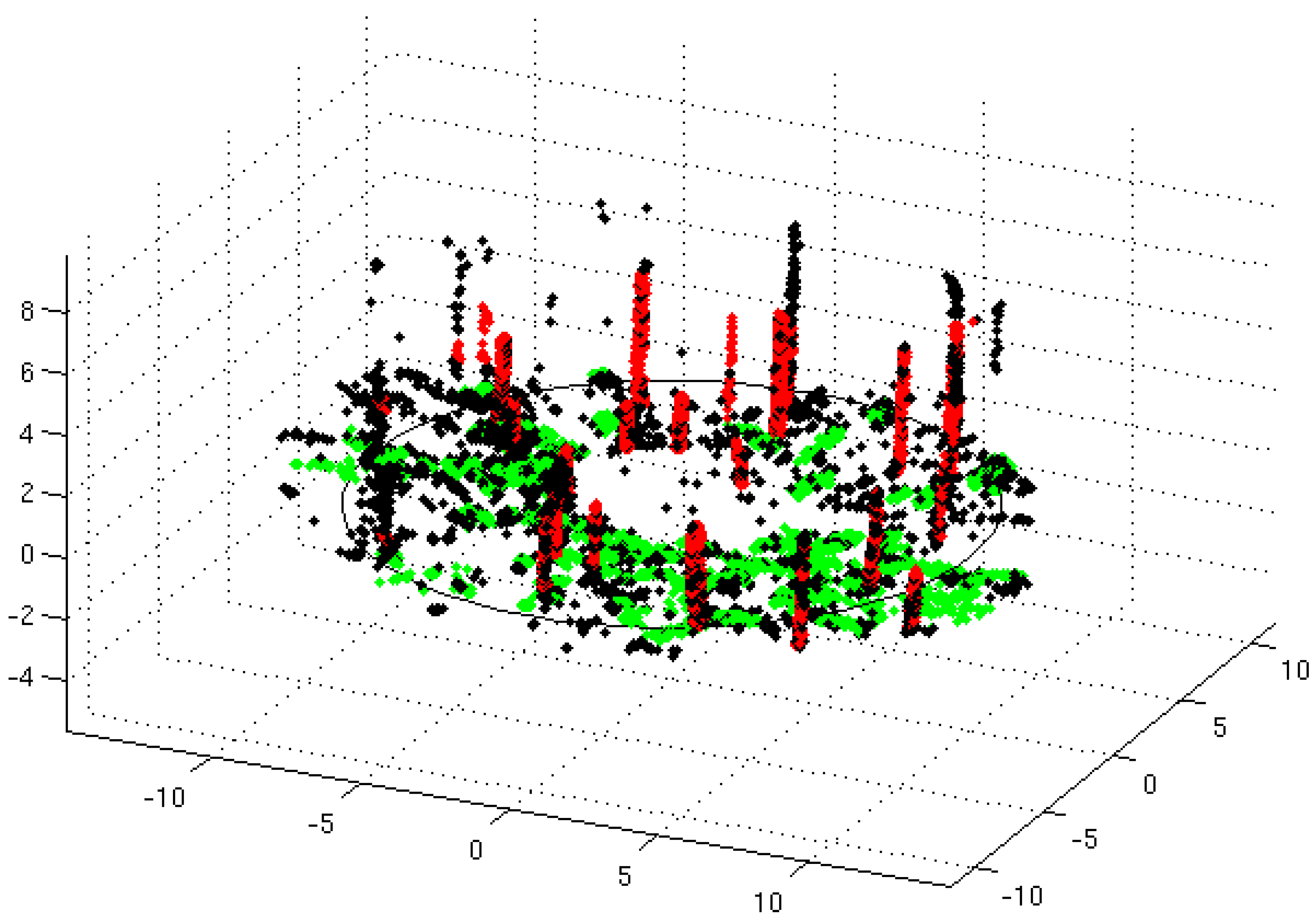
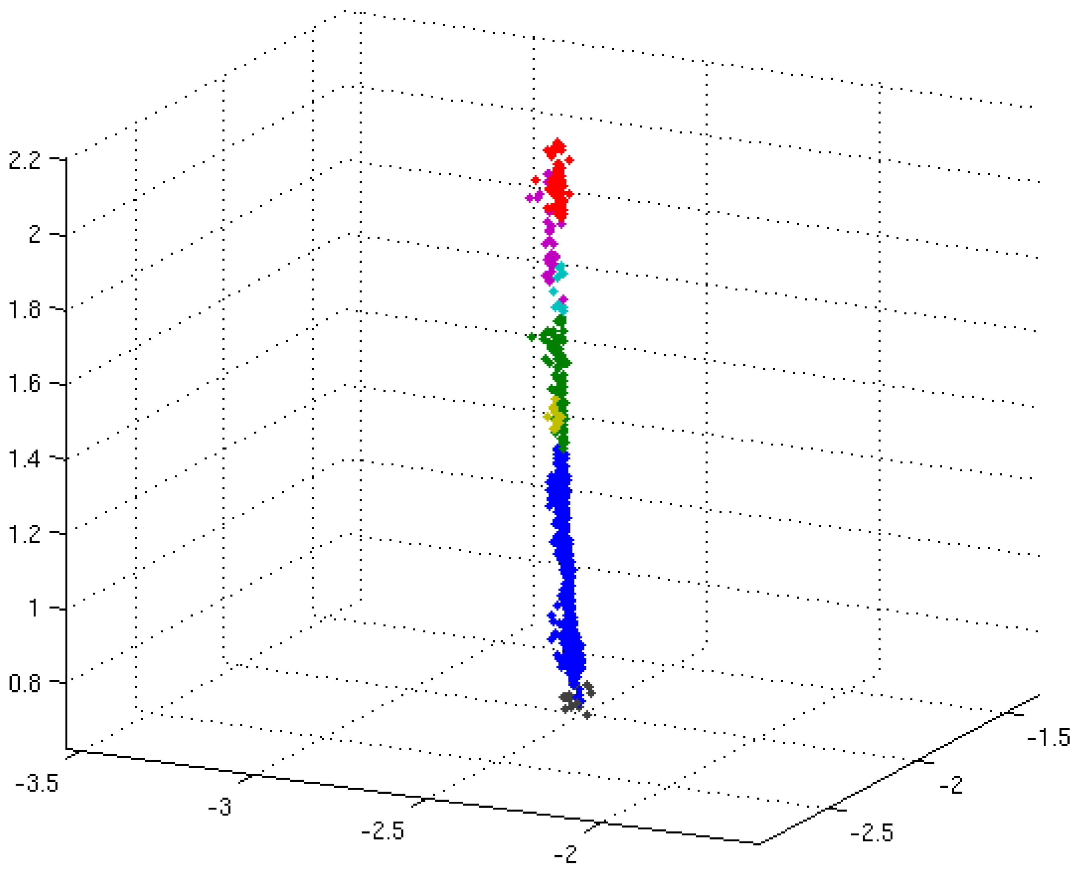
2.5.3. Tree Detection

The tree detection algorithm is similar to the algorithm used in, e.g., Liang et al. [6], Pfeifer et al. [27]. The normal direction of a point describes the orientation of a surface spanned by the point and its neighbors. For each 3D point in the point cloud, the normal direction was calculated from the 18 nearest neighbors by the algorithm in the CGAL (The Computational Geometry Algorithms Library) Library [28]. The co-registered point cloud was segmented into possible stem points, ground points and other points (see Figure 7). Ground points are assumed to have roughly vertical normals, with a normalized vertical component larger than 0.7.

A ground model with 1 m × 1 m cells was calculated from the ground points. The second lowest z-value was assigned to each cell to get a true ground value, not from vegetation or an extreme outlier. For cells without ground points, the mean value of the closest four cells with ground points was used.

Possible stem points were initially selected by assuming that they originate from roughly vertical surfaces, indicated by a small vertical component (below 0.2) in the normal vector. The cloud of possible stem points was further divided into segments representing mostly separate stems using the segmentation algorithm by Rabbani et al. [29]. An angle threshold of 0.3 radians, a residual threshold of 0.1 m and a neighborhood size of 18 points were used.

In a second step, stem segments were connected into stems if they were within a 0.3-m horizontal distance from each other (see Figure 8).

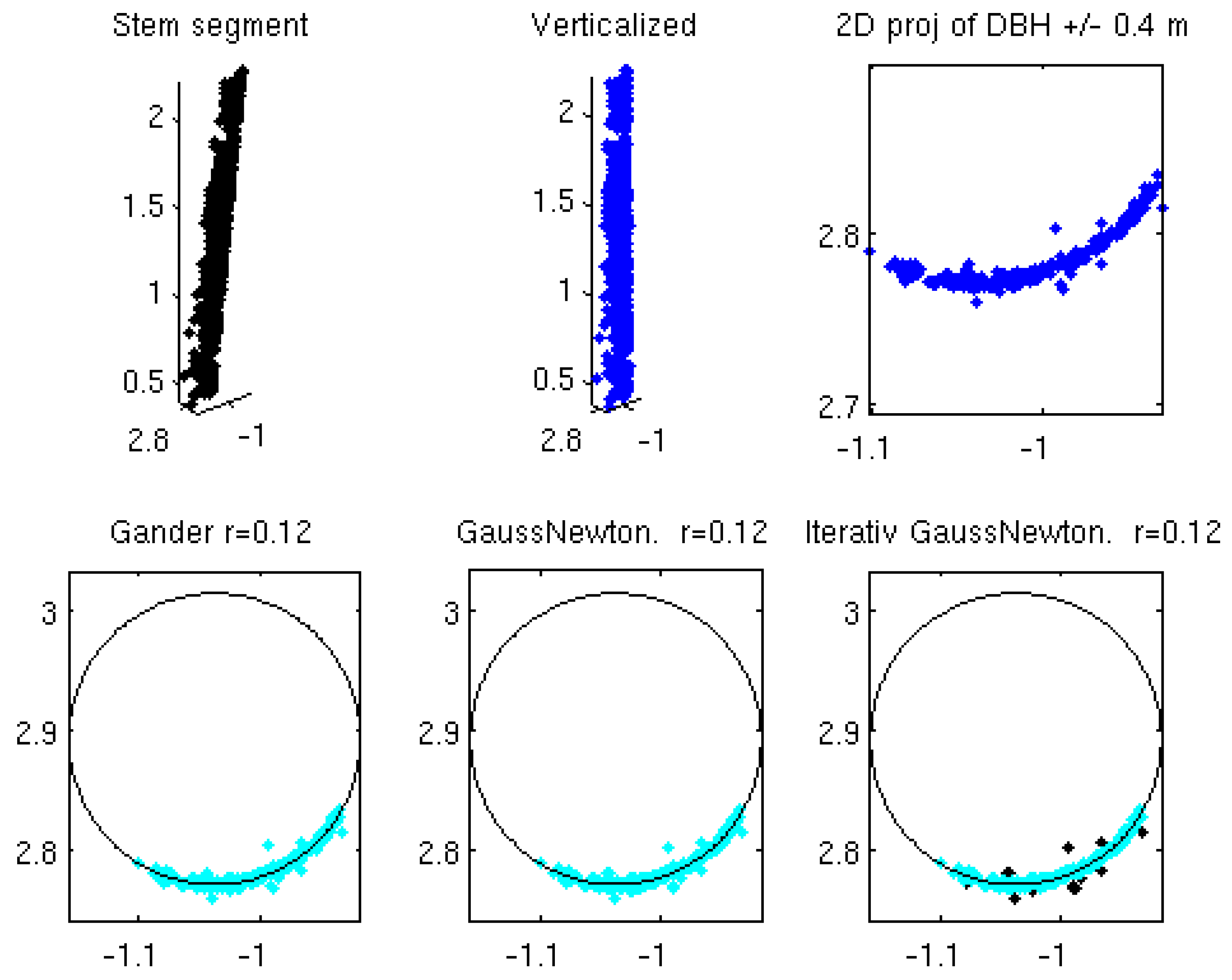
2.5.4. Diameter Estimation

Stem segments that were at least 0.4 m tall and included the breast height were used for further processing. The stem segments were verticalized using principal component analysis (PCA) [24] with constraints to ensure the transformed segment faced the center of the plot (see Figure 9, upper left and center).

A 0.8 m-thick “disc” centered at breast height was cut out from the segment. If the disc contained at least 50 points, the points in the disc were projected to 2D (Figure 9, upper right), and the estimation procedure described below was applied. Otherwise, the stem was classified as “detected, but not possible to estimate”. If the disc contained points from multiple views, only the points from the view with the largest number of points were processed.

2.5.5. Circle Estimation

A two-step method has been used for the circle estimation: (1) an initial estimation of the position and radius from the projected 2D points by the direct method of Gander et al. [30]; and (2) iterative damped Gauss–Newton [21] for least squares adjustment. The adjustment procedure refines the position and radius estimates and also produces an estimate of the coordinate measurement error ${\sigma }_0$ based on the final residual. After convergence, points with a residual larger than 3 ${\sigma }_0$ were assumed to be outliers and were removed from the set, and the Gauss–Newton step was repeated until no outliers remained. The Gauss–Newton estimation reported an error code if the optimization did not converge within 20 iterations. Figure 9 (lower row) shows an example of the different circle estimates.

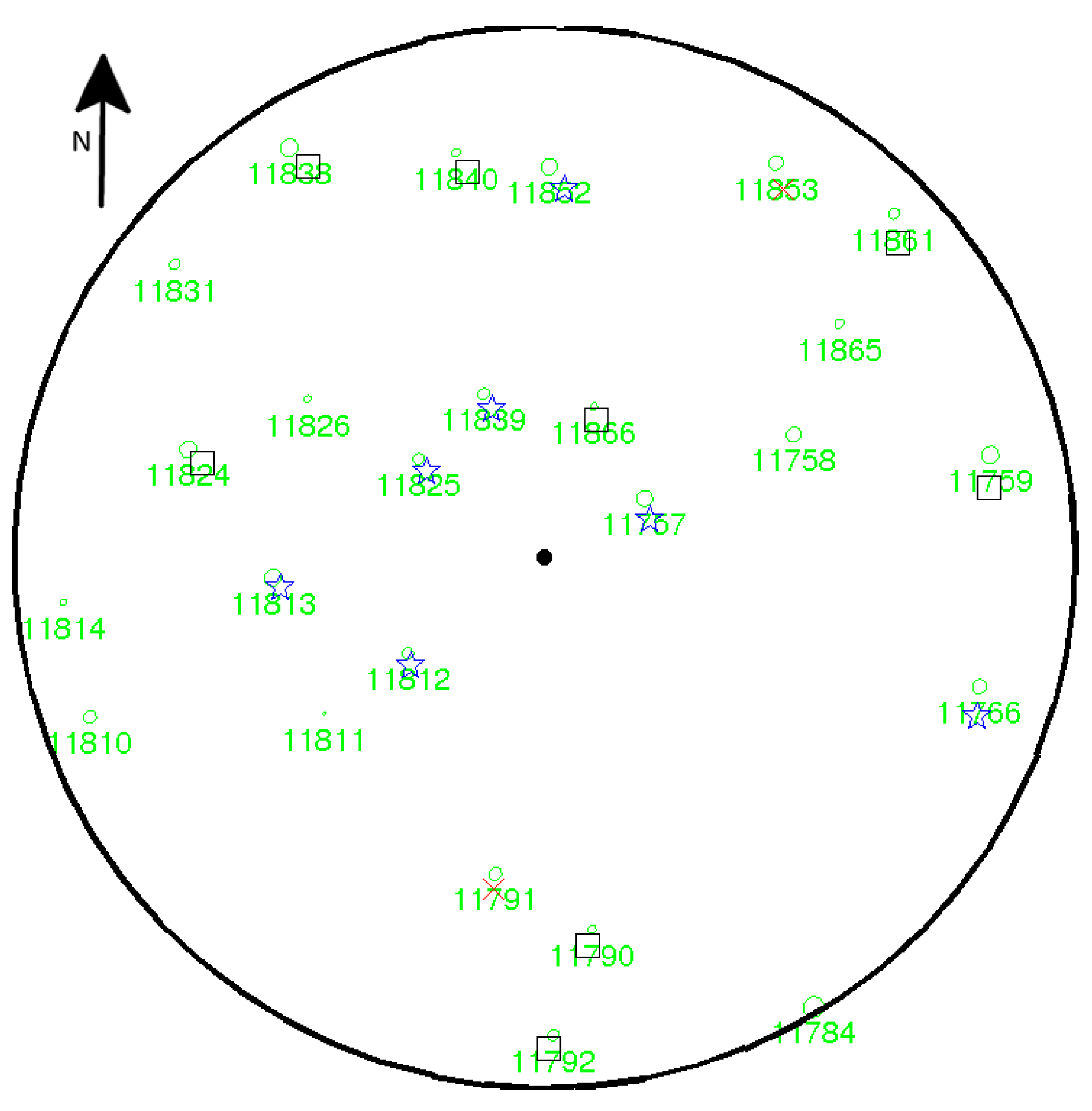
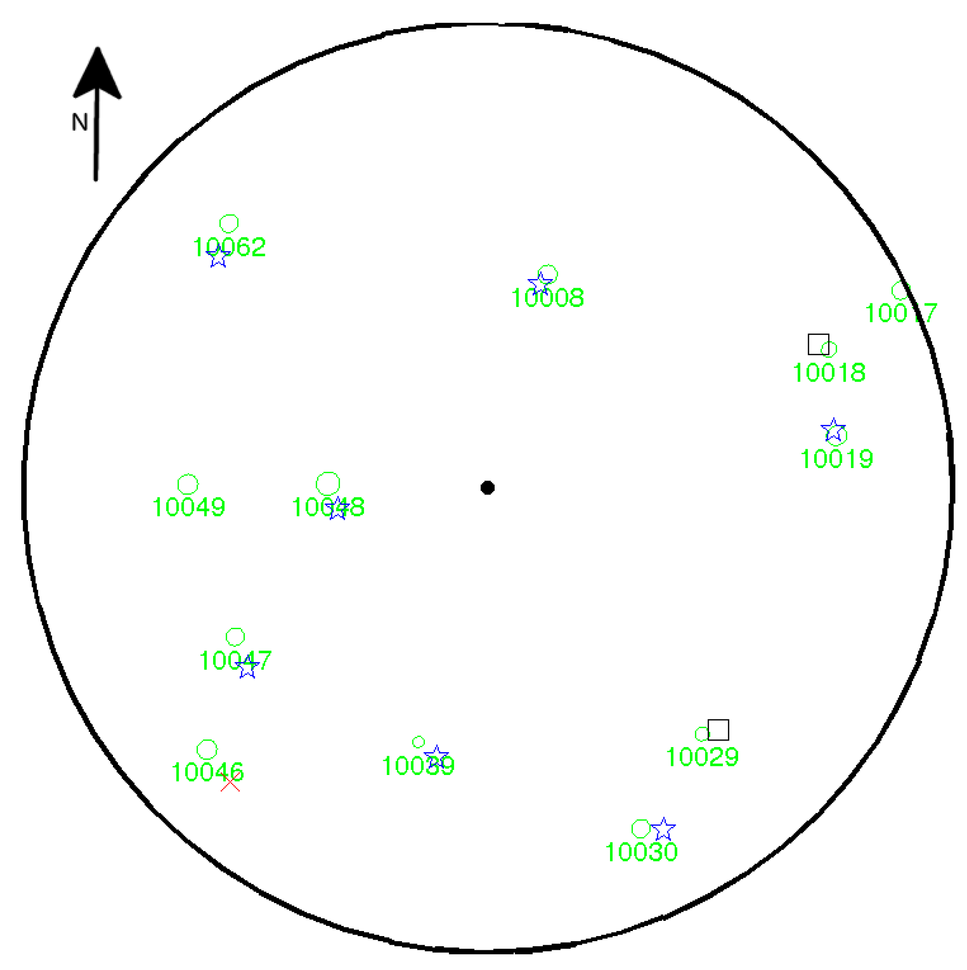
2.5.6. Presentation of Results

Results were presented plot-wise, with a map of detected trees, estimated trees and trees from the ground truth data marked separately. Tables and plots showing the accuracy as evaluated using the ground truth data were also presented.

3. Results

Figure 10 shows a plot of the relative error in the diameter estimate vs. the number of points in the disc. For discs with less than 50 points, the occurrence of gross errors is great. Thus, in the following section, the trees have been classified into four categories:

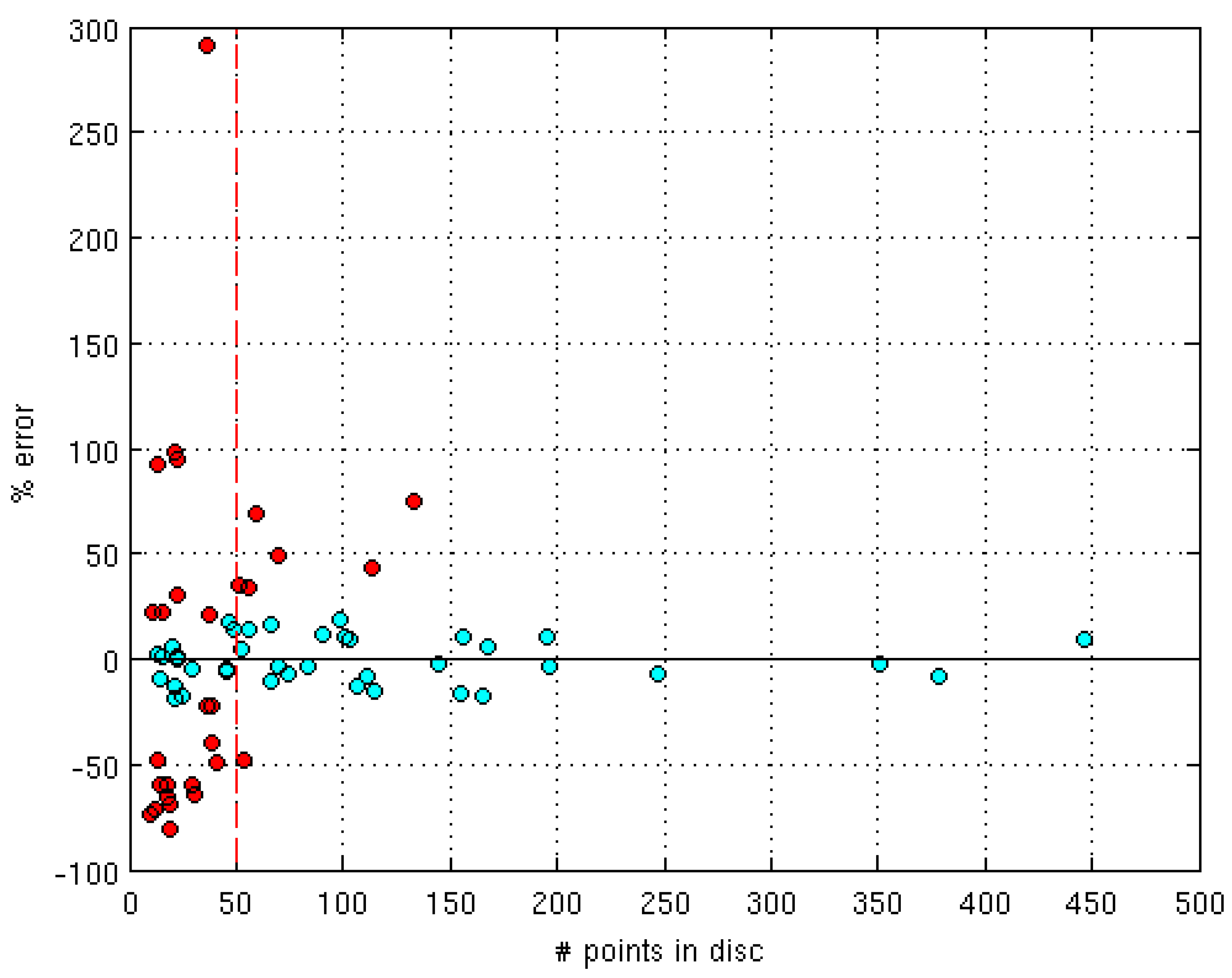
• Correctly estimated tree with a diameter absolute error less than 20%.
• Incorrectly estimated tree with a diameter absolute error of at least 20%.
• Detected tree, where a stem is segmented, but the number of points close to breast height was either too few to be suitable for circle fitting or an error was reported by the circle fitting code. For detected trees, the position was the only reported attribute.
• Invisible tree, where a tree was present in the ground truth, but no corresponding segments were detected in the point cloud.

The results varied among the processed plots. Three plots (165, 167 and 343) had markedly better results than the other three. Visual inspection of the images revealed that the plots with a higher rate of stem detection had clearly visible stems. In contrast, the plots with lower stem detection rates had many twigs on the stems. See Figure 11 and Figure 12 for examples of either case. Plots 165, 167 and 343 were classified as “suitable” for this method, and most of the following results are based on them.

The position of all detected stems in the “suitable” dataset were close to the ground truth values. The position error was typically below 0.5 m and with a systematic shift (Figure 13). The systematic error is expected since the rig was not positioned exactly at the center of each of the field plots. In some cases, a small error was introduced by the co-registration (Figure 14). Within the suitable plots, 76% of the trees were correctly detected and positioned (

Table 2. Result at the plot level. Plots 165, 167 and 343 were sparse with mostly visible stems. Plots 203, 32 and 87 were dominated by spruce with many dry twigs and shrubs on the ground.

Plot No.	# of Trees	Correct	Incorrect	Detected	Invisible
165	25	7	2	8	8
167	22	8	0	10	4
343	12	7	1	2	2
203	34	2	0	9	23
32	29	2	2	7	18
87	38	1	1	13	23
All plots	160	27	6	49	78
Suitable plots	59	22	3	20	14

), and the diameters were estimated for 42% of the trees. The undetected, invisible trees were all obscured by other trees (Figure 13 and Figure 14). The highest detection rate was obtained on Plot 343 with the lowest tree density (0.04 trees/m${}^2$).

The diameter estimation worked well on clearly visible stems. On the suitable plots, the bias was 1.0 cm, and the RMSE was 7.2 cm (

Table 3. Bias and RMSE of diameter estimation at the plot level for all (correct + incorrect) estimated trees; the mean difference (mean diff) of stem positions with the standard deviation (std) at the plot level.

	Diameter (m)		Position (m)
Plot No.	Bias	RMSE	Mean diff	Std
165	0.012	0.095	0.39	0.13
167	−0.005	0.028	0.31	0.11
343	0.023	0.067	0.54	0.25
203	0.024	0.026	0.40	0.1
32	0.040	0.054	0.41	0.08
87	0.110	0.138	0.78	0.01
All plots	0.020	0.074	-	-
Suitable plots	0.010	0.072	-	-

). The errors were slightly larger for trees far away from the camera rig (Figure 15), which is reasonable because of a sparser point cloud and a larger error in each point. A regression line between the estimated diameters and the ground truth diameters is close to a 1:1 line (Figure 16).

4. Discussion

The aim of this work was to develop and validate a method for measurements of DBH and tree positions in forest field plots. The emphasis has been on simplicity and low time requirements on-site. The presented method is based on a multi-camera rig, where the calibration of the cameras and the rig is performed before the matching stage that results in a point cloud. The calibration information is used to reduce the number of false matches. In addition to the standard requirement that the SIFT descriptors should be similar [31], the positions of the SIFT keyframes are required to be close to the epipolar lines emanating from two other, non-collinear cameras. A novel further requirement is that the size and direction of the keyframes must be similar to generate a match. The latter requirement uses the knowledge that the viewing directions from the rig cameras are similar. Finally, as the size of rig baseline is known from calibration, the scaling of the generated point cloud is automatic.

Images were acquired from the center of the plot, looking outwards, and at a nominal angular separation of 30 degrees. The resulting point clouds acquired in different directions were co-registered and segmented. The tree positions and their DBH were estimated on detected stems using a circle fit based on projected 3D points.

The rig was designed with five cameras to be robust with respect to occlusions. Unfortunately, two of the used cameras, both equipped with zoom lenses, were found to be unstable and had to be excluded from the tree estimation process.

The proposed method was validated using manual measurements of tree positions and stem diameters on field plots with different forest conditions. Of the 25 plots, six could be used for validation. Most of the discarded plots had difficult lighting conditions with hard light and dark shadows due to sunny weather. Light overcast weather with dominating ambient light produced the best imagery to work with. However, image matching is still possible in dim forests, if the light is even. Clearly different results were obtained from two different forest types, each represented by three field plots. Three of the validation plots had clearly visible stems and were classified as suitable for our method. The other three plots had a large amount of low branches and twigs near the height for the stem diameter estimates. On the suitable plots, 76% of the trees were detected and positioned with 0% commission errors. The position error was generally below 0.5 m without any extensive attempt to align the position measurements with the ground truth. Tree diameters were further estimated for 42% of the trees with an RMSE of 7.2 cm and a bias of 1.0 cm. On the plot with the lowest tree density, 0.04 trees/m${}^2$, 83% of the trees were detected and positioned, and DBH was estimated on 67% with an RMSE of 6.7 cm and a bias of 2.3 cm.

On some plots, a high proportion of the omission errors was the result of occlusions by other trees along the line of sight from the camera rig. The wide baseline of the rig made it impossible to detect trees at close range. Since a point has to be visible in all cameras, the rig has a blind area up to approximately one meter directly in front of the rig and up to two meters on the sides. For the image acquisition protocol that was used, objects within this distance occluded the scene without producing any 3D points. In those cases, the point cloud was seriously limited in some directions.

The rig was designed with five non-collinear cameras for a number of reasons: Requiring more than two cameras per match would reduce the number of false matches compared to two cameras. Furthermore, having two extra cameras would increase the robustness with respect to occlusions. Variable baseline lengths would allow for point detection both at close and long ranges, and the rig-combined field of view would allow for co-registration between exposures taken 30 degrees apart. The loss of the two extra cameras removed several of these potential advantages. The rig was left with a narrow overlapping field straight ahead and produced a point cloud of lower density compared to a five-camera rig. The overlapping areas between subsequent views became small and made the co-registration difficult. In hindsight, the inclusion of zoom lenses into the rig design must be considered a mistake.

Photogrammetric measurements of trees are a developing field. Most of the recent studies are based on single-camera techniques. Although several techniques have published impressive reconstruction results, almost all methods were evaluated in park-like conditions, i.e., from multiple viewing directions, effectively free-standing trees, and evaluated on a few trees only. We argue that the imaging environment in a real forest is significantly more challenging due to the lighting conditions, higher tree density and occlusions by branches, shrubs, etc. To our knowledge, the only published camera-based method that has been evaluated in a natural forest is the method of Liang et al. [15], also described in the comparative study Liang et al. [10]. The method was evaluated on a single 30-by-30 m field plot with 25 trees, i.e., with a tree density of 35%–73% of our suitable plots. Using the full dataset of 973 images acquired around and inside the plot (called Method I in Liang et al. [10]), they reported a detection rate of 88%, an RMSE of 2.39 cm with a commission error of 12%. The image dataset was augmented by manual field measurements. Using a smaller 97-image subset with an acquisition protocol similar to ours (Method III in Liang et al. [10]), the results were a 60% tree detection rate, an RMSE of 6.46 cm and a bias of −0.15 cm. The reported image acquisition time was between 15 and 45 min, depending on the photographic path. Another study by Rodríguez-García et al. [17] used a stereoscopic purpose-built fisheye configuration and was validated on a single plantation plot of Eucalyptus trees with a comparable density to our suitable plots. The images were acquired from a single viewpoint on the scene. The reported RMSE for tree positions and DBH were 23 cm and 1.51 cm, respectively, for trees closer than 8 m to the cameras. No detection rate, bias, nor time on-site was reported.

In contrast, a number of TLS methods have been evaluated in a forest environment. The single-scan study Liang et al. [32] was evaluated on nine field plots with 289 trees and reported a 73% detection rate with 15% commissions. Neither RMSE, bias nor time on-site were reported. Another single-scan study [7], which used the same test site as this study, was validated on 16 field plots with a 20-m radius. The detection rate within 10 m from the scanner was 87% with a commission rate of 6%. DBH was estimated with an RMSE of 3.9 cm and bias of 1 cm. The multi-scan TLS method in [10] was evaluated on the same plot as Liang et al. [15]. The detection rate was 100% with 8% commission, an RMSE of 3.36 cm and a bias of 0.28 cm. The reported time on-site was about one hour for five scans, i.e., 12 min per scan.

The multi-scan TLS and the 973-image methods were both considered intractable due to about a one-hour data acquisition time per field plot and were excluded from further comparisons. Compared to the best TLS method [7], the results for our method are inferior, except for the commission errors. Furthermore, our test set is smaller. However, the TLS hardware cost is about 4–5-times higher [10], and the time on-site is about six-times higher. If an average car-to-field plot transportation time of 20 min is included, our time advantage is reduced, but TLS would still require about 50% more time per field plot.

Based on our suitable plots, our results are inferior to the single-camera Method III of Liang et al. [10] that was evaluated on a significantly sparser plot. Furthermore, our hardware cost is 7–10-times higher. If the comparison is instead based on the plot with the lowest tree density, our method has a higher detection rate, a comparable RMSE, but a higher bias. In either case, our time advantage is similar to that of TLS. Since the required time on-site for our proposed method is only two minutes, it is reasonable to assume that our method is significantly faster than manual inventory methods, especially if the time to measure tree positions is included.

Automatic detecting and estimating of trees on field plots is a difficult problem. The results depend both on environmental conditions and methodological considerations. The environmental factors include tree density, the amount of occlusions by branches and shrubs and imaging conditions due to weather. The methodological factors include choices of the hardware and data acquisition protocol and acceptable time on-site. If an automatic method is to be deployed at large scale, the cost of the equipment and data acquisition must be reasonable, while the results must be acceptable. Currently, TLS methods produce the best results, although with a high equipment cost and/or a long data acquisition time. Camera-based methods, either single-camera or rig-based, currently offer a less expensive alternative, both in terms of equipment and data acquisition cost. Another advantage of camera-based methods is the automatic photo-documentation that can be useful for further interpretation and additional survey of the environment.

The advantage of single-camera methods compared to our rig-based method is less bulky equipment and lower equipment cost. However, as single-camera methods estimate the relationship between the images during the matching process, a more complicated and time-consuming image acquisition protocol on-site is required. Furthermore, published single-camera methods require added measurement to establish the scale of the resulting point cloud and have so far only been validated on plots with low tree density. A larger amount of photogrammetric knowledge may also be required by the field staff to avoid unfavorable image configurations, such as almost collinear camera positions. Using a rig can reduce such concerns and enable a faster and less complex imaging protocol, as part of the photogrammetric knowledge is included in the rig design.

Our image acquisition protocol specified that all images should be taken at a single station at the center of the plot. The advantages were simplicity and acquisition speed. However, for some plots with trees close to the plot center, the close-range tree trunks occluded a large part of the plot. As a future investigation, we suggest extending the image acquisition protocol to 2–3 stations and reducing the angular separation to 20 degrees to ensure adequate overlap between views. If the image stations are kept close to the plot center, the added time on-site should stay below five minutes.

The accuracy of the stem diameter estimations was clearly dependent on the number of 3D points on the tree stems, especially near breast height. The number of points was a function of the thresholds used in the algorithm used for the 3D point clouds’ construction. A higher number of 3D points could have been produced with lower thresholds, but the point cloud would include more false points. On several of the detected tree stems whose diameter could not be estimated, the detected points were clustered above and below breast height with few points usable for DBH estimation. One way to estimate the diameter of such partly-occluded trees could be to fit a tapered cylinder to the detected point clusters.

Other future investigations include a comparison between a three-camera and five-camera rig to allow for a less expensive, smaller and lighter rig, as well as a study of exposure parameters to reduce the weather sensitivity. A potential of our method is that the rig could be useful for forest inventory using a transect method where the trees along a path are measured, such as in Hessenmöller et al. [33]. The co-registration methods used in this study are easy to apply to a stop and go acquisition scheme, where an image set is acquired for every few steps.

In summary, the automation potential, the non-requirement of site modification and the low cost and low time on-site properties of the proposed method make it a viable method for the estimation of stem diameters on low tree density field plots. However, the image acquisition scheme could be optimized to achieve a higher detection rate and estimation accuracy and to work on plots with higher tree densities. The time spent on inventory can be significantly reduced compared to manual field measurements, at the cost of some omitted trees and reduced precision. Stem positions, which can be useful for the training of remote sensing methods, and photo documentation are additional values that this method provides.

References

- Riksskogstaxeringen. Available online: http://www.slu.se/sv/centrumbildningar-och-projekt/ riksskogstaxeringen/hur-vi-jobbar/ (accessed on 1 February 2016).
- Olofsson, K.; Lindberg, E.; Holmgren, J. A Method for Linking Field-surveyed and Aerial-detected Single Trees using Cross Correlation of Position Images and the Optimization of Weighted Tree List Graphs. In Proceedings of the SilviLaser, Edinburgh, UK, 17–19 September 2008; pp. 95–104.
- Lindberg, E.; Holmgren, J.; Olofsson, K.; Olsson, H. Estimation of Stem Attributes using a Combination of Terrestrial and Airborne Laser Scanning. In Proceedings of the SilviLaser, Freiburg, Germany, 14–17 September 2010; pp. 1917–1031.
- Vauhkonen, J.; Maltamo, M.; McRoberts, R.E.; Næsset, E. Forestry Applications of Airborne Laser Scanning; Springer: Netherlands, Netherlands, 2014; Chapter 4.3.3; p. 74. [Google Scholar]
- Clark, N.A.; Wynne, R.H.; Schmoldt, D.L. A Review of Past Research on Dendrometers. For. Sci. 2000, 46, 570–576. [Google Scholar]
- Liang, X.; Litkey, P.; Hyyppä, J.; Kaartinen, H.; Vastaranta, M.; Holopainen, M. Automatic Stem Mapping Using Single-Scan Terrestrial Laser Scanning. IEEE Trans. Geosci. Remote Sens. 2012, 50, 661–670. [Google Scholar] [CrossRef]
- Olofsson, K.; Holmgren, J.; Olsson, H. Tree Stem and Height Measurements using Terrestrial Laser Scanning and the RANSAC Algorithm. Remote Sens. 2014, 6, 4323–4344. [Google Scholar] [CrossRef]
- Ducey, M.J.; Astrup, R. Adjusting for nondetection in forest inventories derived from terrestrial laser scanning. Can. J. Remote Sens. 2013, 39, 410–425. [Google Scholar]
- Liang, X.; Hyyppä, J. Automatic stem mapping by merging several terrestrial laser scans at the feature and decision levels. Sensors 2013, 13, 1614–1634. [Google Scholar] [CrossRef] [PubMed]
- Liang, X.; Xinlian, L.; Yunsheng, W.; Anttoni, J.; Antero, K.; Harri, K.; Juha, H.; Eija, H.; Jingbin, L. Forest Data Collection Using Terrestrial Image-Based Point Clouds From a Handheld Camera Compared to Terrestrial and Personal Laser Scanning. IEEE Trans. Geosci. Remote Sens. 2015, 53, 5117–5132. [Google Scholar] [CrossRef]
- Reidelstürz, P. Forstliches Anwendungspotential der terrestrisch—Analytischen Stereo- photogrammetrie. Ph.D. Thesis, der Albert-Ludwigs-Universität Freiburg, Breisgau, Germany, 1997. [Google Scholar]
- Fürst, C.; Nepveu, G. Assessment of the assortment potential of the growing stock—A photogrammetry based approach for an automatized grading of sample trees. Ann. For. Sci. 2006, 63, 951–960. [Google Scholar] [CrossRef]
- Dick, A.R.; Kershaw, J.A.; MacLean, D.A. Spatial Tree Mapping Using Photography. N. J. Appl. For. 2010, 27, 68–74. [Google Scholar]
- Berveglieri, A.; Oliveira, R.A.; Tommaselli, A.M.G. A feasibility study on the measurement of tree trunks in forests using multi-scale vertical images. Int. Archives Photogrammetry Remote Sens. Spat. Inf. Sci. 2014, XL-5, 87–92. [Google Scholar] [CrossRef]
- Liang, X.; Jaakkola, A.; Wang, Y.; Hyyppä, J.; Honkavaara, E.; Liu, J.; Kaartinen, H. The Use of a Hand-Held Camera for Individual Tree 3D Mapping in Forest Sample Plots. Remote Sens. 2014, 6, 6587–6603. [Google Scholar] [CrossRef]
- Gatziolis, D.; Lienard, J.F.; Vogs, A.; Strigul, N.S. 3D Tree Dimensionality Assessment Using Photogrammetry and Small Unmanned Aerial Vehicles. PLoS ONE 2015, 10, e0137765. [Google Scholar] [CrossRef] [PubMed]
- Rodríguez-García, C.; Montes, F.; Ruiz, F.; Cañellas, I.; Pita, P. Stem mapping and estimating standing volume from stereoscopic hemispherical images. Eur. J. For. Res. 2014, 133, 895–904. [Google Scholar] [CrossRef]
- Forsman, M.; Börlin, N.; Holmgren, J. Estimation of tree stem attributes using terrestrial photogrammetry. Int. Archives Photogrammetry Remote Sens. Spat. Inf. Sci. 2012, XXXIX-B5, 261–265. [Google Scholar] [CrossRef]
- Easyrig 2.5. Available online: http://www.easyrig.se/product/easyrig-2-5.
- Börlin, N.; Grussenmeyer, P. Camera Calibration using the Damped Bundle Adjustment Toolbox. In Proceedings of the ISPRS Technical Commission V Symposium, Riva del Garda, Italy, 23–25 June 2014; 2014; Volume II-5, pp. 89–96. [Google Scholar]
- Börlin, N.; Grussenmeyer, P. Bundle Adjustment With and Without Damping. Photogramm. Rec. 2013, 28, 396–415. [Google Scholar] [CrossRef]
- Vedaldi, A.; Fulkerson, B. VLFeat: An Open and Portable Library of Computer Vision Algorithms. Available online: http://www.vlfeat.org/ (accessed on 3 March 2016).
- Hartley, R.I.; Zisserman, A. Multiple View Geometry in Computer Vision, 2nd ed.; Cambridge University Press: Cambridge, UK, 2003; ISBN 0521540518. [Google Scholar]
- Chris McGlone, J.; Mikhail, E.M.; Bethel, J.S.; American Society for Photogrammetry and Remote Sensing. Manual of Photogrammetry; American Society for Photogrammetry and Remote Sensing: Bethesda, Maryland, 2004. [Google Scholar]
- Fischler, M.A.; Bolles, R.C. Random Sample Consensus: A Paradigm for Model Fitting with Applications to Image Analysis and Automated Cartography. Commun. ACM 1981, 24, 381–395. [Google Scholar] [CrossRef]
- Söderkvist, I.; Wedin, P.A. Determining the Movements of the Skeleton Using Well-Configured Markers. J. Biomech. 1993, 26, 1473–1477. [Google Scholar] [CrossRef]
- Pfeifer, N.; Gorte, B.; Winterhalder, D. Automatic Reconstruction of Single Trees from Terrestrial Laser Scanner Data. In Proceedings of the 20th ISPRS Congress, Istanbul, Turkey, 12–23 July 2004.
- The CGAL Project. CGAL User and Reference Manual, 4.7 ed.; CGAL Editorial Board, 2015. [Google Scholar]
- Rabbani, T.; van den Heuvel, F.; Vosselmann, G. Segmentation of point clouds using smoothness constraint. Int. Arch. Photogram. Remote Sens. Spatial Inf. Sci. 2006, 36, 248–253. [Google Scholar]
- Gander, W.; Golub, G.H.; Strebel, R. Least-squares fitting of circles and ellipses. BIT 1994, 34, 558–578. [Google Scholar] [CrossRef]
- Lowe, D.G. Distinctive Image Features from Scale-Invariant Keypoints. Int. J. Comput. Vis. 2004, 60, 91–110. [Google Scholar] [CrossRef]
- Liang, X.; Litkey, P.; Hyyppä, J.; Kaartinen, H.; Kukko, A.; Holopainen, M. Automatic plot-wise tree location mapping using single-scan terrestrial laser scanning. Photogramm. J. Finland 2011, 22, 37–48. [Google Scholar]
- Hessenmöller, D.; Elsenhans, A.S.; Schulze, E.D. Sampling forest tree regeneration with a transect approach. Ann. For. Res. 2013, 56, 3–14. [Google Scholar]