Assessment of Forest Structure Using Two UAV Techniques: A Comparison of Airborne Laser Scanning and Structure from Motion (SfM) Point Clouds

Abstract

This study investigates the potential of unmanned aerial vehicles (UAVs) to measure and monitor structural properties of forests. Two remote sensing techniques, airborne laser scanning (ALS) and structure from motion (SfM) were tested to capture three-dimensional structural information from a small multi-rotor UAV platform. A case study is presented through the analysis of data collected from a 30 × 50 m plot in a dry sclerophyll eucalypt forest with a spatially varying canopy cover. The study provides an insight into the capabilities of both technologies for assessing absolute terrain height, the horizontal and vertical distribution of forest canopy elements, and information related to individual trees. Results indicate that both techniques are capable of providing information that can be used to describe the terrain surface and canopy properties in areas of relatively low canopy closure. However, the SfM photogrammetric technique underperformed ALS in capturing the terrain surface under increasingly denser canopy cover, resulting in point density of less than 1 ground point per m² and mean difference from ALS terrain surface of 0.12 m. This shortcoming caused errors that were propagated into the estimation of canopy properties, including the individual tree height (root mean square error of 0.92 m for ALS and 1.30 m for SfM). Differences were also seen in the estimates of canopy cover derived from the SfM (50%) and ALS (63%) pointclouds. Although ALS is capable of providing more accurate estimates of the vertical structure of forests across the larger range of canopy densities found in this study, SfM was still found to be an adequate low-cost alternative for surveying of forest stands.

1. Introduction

Forest structure refers to the spatial arrangement of the components of a forest ecosystem, and describes properties such as the horizontal and vertical distribution and abundance of vegetative elements [1]. Measurements of forest structure can be used as an indicator of biodiversity [2], but also to derive estimates of biomass [3]. Capturing the variability of structural properties across a forested landscape has conventionally employed on-ground measurements conducted within a small set of sample plots. These measurements are, however, labour intensive and their ability to characterise landscape level variables is limited by the cost of establishing a sufficient number of sample plots capturing the existing landscape variability.

Remote sensing can complement existing ground-based techniques, providing spatially representative characteristics of investigated forest stands in a more efficient manner. Data captured over varying spatial, spectral, and temporal scales has been shown to contain information, which can be used to measure and monitor various aspects of a complex forest structure [4,5,6]. Advances in acquisition of this information have led to high spatial resolution three-dimensional (3D) remote sensing becoming an important tool in forest modelling [5,6,7,8,9].

Small-size unmanned aerial vehicles (mini-UAVs of less than 5 kg) represent a low-cost remote sensing alternative to airborne and satellite platforms that, when equipped with sensors, can produce cost-effective data at local scales (e.g., for areas the size of traditional forest plots up to areas of several km²) with an unrivalled combination of spatial and temporal resolution [10]. The fine-scale data captured by mini-UAVs has been used, for instance, to measure biophysical properties of citrus plantations [11] or to assess health of Antarctic moss [12,13]. Equipping mini-UAVs with sensors capable of detecting 3D structure has led to the systems being increasingly used to provide an understanding of the structure and variability of forests [14,15,16,17].

Two approaches have been developed in order to capture the 3D structure of forest stands from sensors on-board UAVs: (i) the use of laser scanners [15,18] and (ii) the use of computer vision algorithms and imagery captured from digital still cameras [14,16]. Laser scanning systems measure the time of flight of an emitted laser pulse to be reflected off of an intercepted feature and return to the sensor, from which a range measurement can be calculated. Point clouds derived from images are generated with computer vision/photogrammetry techniques, such as structure from motion (SfM). SfM operates under the principles of traditional stereoscopic photogrammetry, using well defined geometrical features captured in multiple images from different angular viewpoints to generate a 3D point cloud [19]. SfM has built onto tradional stereoscopic techniques as a result of advances in computer vision algorithms, such as the Scale Invariante Feature Transform (SIFT), and parallel bundle adjustments on graphics processing units (GPUs). These developments have made it possible to match image features in many overlapping photographs (100s–1000s) acquired from different angles, which makes SfM ideally suited to photograms acquired from small UAVs [11,12,14]. Point clouds generated with both LiDAR and SfM technologies have been demonstrated to provide information representative of forest attributes including height, canopy dimensions, and biomass at both the area and tree levels [14,15,20,21].

Comparisons between ALS data collected from manned aircraft and point clouds produced from UAV collected photographs [16], but also data captured solely from manned aircraft [8,9,22,23,24], have shown that differences occur at all stages of the data processing workflow, i.e., from data collection through the generation of metrics to the assessment of object structure. Notably, it has been shown that imagery can capture spectral information that in some cases produces a more detailed representation of the upper canopy [14]. Imaging technology, however, does not provide the same level of penetration into the canopy as laser scanning, and therefore cannot deliver the same level of information on vertical stratification of vegetation layers and the terrain. Furthermore, because ground terrain needs to be visible from multiple locations in order to estimate its 3D location, several studies have highlighted that the accurate generation of canopy height information from SfM often requires the use of a digital terrain model (DTM) supplied from an external source [9,14,16].

The objective of this study is to provide a comparison of ALS and SfM point clouds captured from a small-UAV platform across a case study forest plot with varying levels of canopy cover. We will assess the differences in the data acquisitions, processing workflows, and forest structure assessment capabilities of the 3D point clouds produced with both these techniques. The study aims to provide insight into the advantages and disadvantages of both practices for the on-demand collection of high-resolution 3D structural information about forest canopies useable in local scale mapping and forest monitoring applications.

2. Materials and Methods

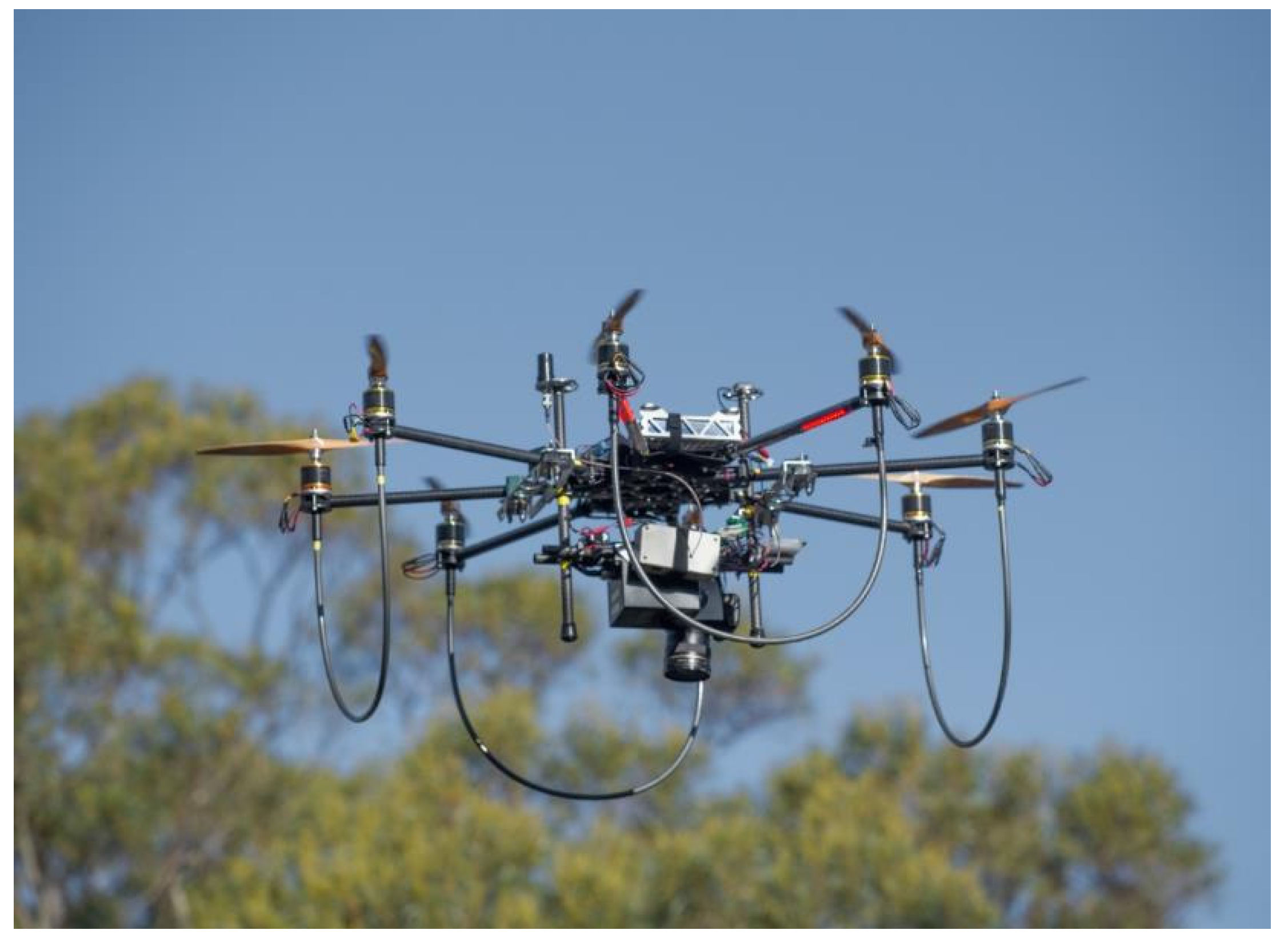
2.1. Airborne Equipment and Processing Software

The mini-UAV used in this study was a multi-rotor Droidworx Skyjib Oktokopter equipped with Mikrokopter electronics (Figure 1). This multi-rotor UAV has eight brushless motors that operate at different rotor speeds to achieve stable directional flight. In order to reduce the effect of airframe vibrations on the sensors, the whole sensor payload weighing approximately 3 kg was mounted on a rigid frame isolated from the motors using four silicon mounts. Colour red-green-blue (RGB) photographs were captured with a Canon 550D digital single lens reflex (DSLR) camera (18 Megapixel, 5184 × 3456 pixels, 20 mm focal length and a field of view of 58 degrees across-track and 41 degrees along-track) at a rate of approximately 3.5 Hz. Laser scanning data was captured with an Ibeo LUX laser scanner, which measures up to three laser returns per pulse, and was setup to collect observations within a scan angle range of ±30°. This discrete-return small footprint scanner operates at a wavelength of 965 nm and utilises four parallel scanning layers and emitting ~22,000 pulses per second. The scanner has a transversal across-track beam divergence of 0.8° and a perpendicular along-track divergence of 0.08°. A detailed description of the UAV laser scanning system can be found in Wallace et al. [18]. The mini-UAV system used in this study was designed to accommodate the laser scanner and the DSLR camera simultaneously.

The on-board positioning and orientation sensors consisted of a Novatel dual frequency global positioning system (GPS) receiver and a Microstrain microelectromechanical-based inertial measurement unit (IMU). The GPS receiver was used as the master timing unit recording both the starting time of each laser scan and the time of exposure of every photograph [13,18]. GPS data was post-processed in GrafNav software utilising a short baseline differential solution to determine the position of the UAV with an accuracy of 2 to 4 cm at 20 Hz and at the start of each scan (occurring at a rate 12 Hz). GPS base station observations were recorded with a Leica Viva GPS receiver located approximately 60 m from the study area during the UAV flight operations.

The laser scanner data was georeferenced based on a Sigma Point Kalman Smoother (SPKS). The reader is referred to Wallace et al. [18] for a detailed description and accuracy assessment of the SPKS algorithm. In summary, the SPKS combines position and velocity of the mini-UAV as measured by the GPS and rotational velocity and acceleration from the IMU to optimally estimate the position and attitude of the UAV platform. This information is then combined with the range, scan angle, and layer angle measured by the laser scanner to produce a fully georeferenced point cloud in the Log ASCII Standard (LAS) file format.

The Agisoft Photoscan Professional v1.0.0 (www.agisoft.com) software (Agisoft LLC, St. Petersburg, Russia), that implements modern SfM algorithms, was used to generate a point cloud from the RGB photographs. Detailed descriptions of the Photoscan workflow can be found in [12,13,25]. In short, Photoscan initially detects tens of thousands of features in each image, which are then matched between the images. An iterative bundle adjustment is then applied to estimate the 3D positions of the matched features, and the positions and orientations of the camera. This information is used in a dense multi-view reconstruction of the scene geometry from the aligned images. Rather than using ground control points (GCP) to georeference the created scene, we applied a direct georeferencing technique based on the GPS-measured camera positioning as described in Turner et al. [13]. This processing step enabled us to compare directly the SfM and ALS point cloud accuracies. Throughout the Photoscan workflow we used the high accuracy setting, i.e., for point detection, construction of the dense point cloud, and the geometry build phase of processing. After initial alignment the inbuilt function in Photoscan was used to optimise the position of the sparse point cloud, based on the accurate camera positions as recorded by the onboard GPS. Accuracy testing discovered that the positional accuracy of the final point cloud was of the same order as the accuracy of the GPS used to measure the camera positions, as reported in Turner et al. [13].

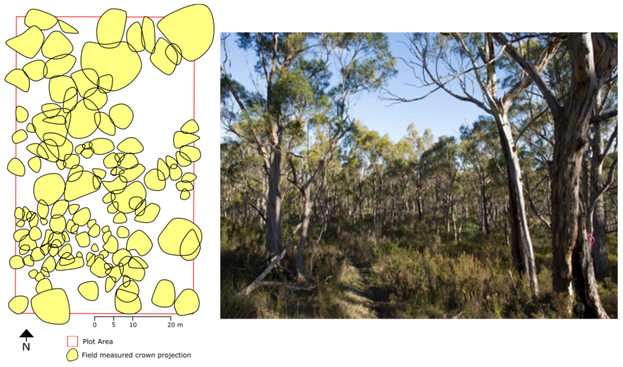
2.2. Study Area and Ground/Airborne Data Collection

The study area is a patch of native dry sclerophyll eucalypt forest located southeast of Hobart, Tasmania, Australia. A target area, represented by a 30 × 50 m rectangular plot, was chosen to capture a wide range of stem densities and canopy cover variability in a single UAV flight. The plot consisted of Eucalyptus pulchella trees of varying age and ranging in height from 4.7 m to 16.2 m. The understory in the northeast corner consisted of low to medium height (0.5–2 m) shrubs, covering about 80% of the ground (Figure 2). The understory in the remainder of the plot consisted of native grassland between 0.3 and 0.5 m in height.

Field measurements of tree structural characteristics were collected using a FieldMap forest mapping system produced by IFER Ltd. The FieldMap system utilises a laser rangefinder combined with an inclinometer and electronic compass, all mounted on a tripod and connected via Bluetooth to a field computer. The location, tree height, crown projection, crown base height, and trunk diameter at breast height (DBH) of every tree were measured and stored in a geographical relational database. DBH measurements were taken using an electronic caliper. Tree locations and heights were measured from survey stations coordinated using offsets from two GPS control points strategically distributed throughout the plot. From these stations, the inclination to the tree top, the stem base, and the distance to a tree were measured using a laser range finder (TruPulse, Laser Technology) from which tree heights were derived. The position of each station was recorded in local Cartesian coordinates and later transformed into MGA95 projection system coordinates using locally collected post-processed survey-grade GPS data. All measurements were directly visualised as a digital map on the field computer screen in real-time, which allowed for visual checking and immediate corrections of data acquisition errors.

Dual frequency GPS measurements were also used to geolocate corners of the study plot and 24 GCP targets randomly placed throughout the plot in areas with limited canopy cover. The GCPs consisted of 14 highly reflective ground targets, detectable in both the laser scanning data and the RGB photographs, and 10 photogrammetric targets detectable in RGB photographs. They were coordinated using a real time kinematic (RTK) GPS technique, which due to limited sky view produced a positional error within ±0.05 m horizontally and ±0.20 m vertically. The same base station was used for the UAV and the field survey. The base station was logging raw data at 20 Hz for post-processing of the UAV position, and the base station was broadcasting a 1 Hz signal for the RTK field survey of the GCPs. The plot corner coordinates were used to georeference the FieldMap measured tree locations and crown projections.

ALS data and RGB photographs of the study plot were captured simultaneously by flying the mini-UAV at a flight altitude of 30 m above the ground level along four North-South transects spaced approximately 10 m apart. The flight was undertaken in April during a period of clear skies and minimal winds at approximately solar noon. This resulted in a laser scan swath width of 34 m for each overpass and an overlap between swaths of approximately 24 m. Trimming unwanted photos from ascent and descent resulted in a total of 425 images (>95% forward and on average 66% side overlap) that were used in the SfM processing workflow.

2.3. Point Cloud Pre-Processing

Both the ALS and SfM acquired point clouds were exported to the LAS format and points representing the ground surface were identified using the Lasground tool of the Lastools software [26]. Several combinations of processing options of the Lasground tool were tested. The best results, a sufficiently dense ground representation with minimal non-ground points as determined by visual inspection, were achieved with a step size of 3 m, an offset of 0.05 m and a spike threshold of 1 m for both the ALS and SfM point clouds. These settings were used to identify ground points, which were then interpolated using a triangular irregular network (TIN) into a DTM of 10 cm pixel-size for both the ALS (DTM_ALS) and SfM (DTM_SfM) point clouds. These DTMs were then used to compute the above-ground height of all non-ground points in the respective point clouds.

2.4. Extraction of Forest Structural Attributes

The assessment of the data produced by the two techniques is compared by extracting information describing the following four important forest structural properties:

• the terrain surface;
• the horizontal distribution of the canopy;
• the vertical stratification of vegetation within the forest;
• the height, location and crown area of individual stems.

In order to assess the information content of each point cloud in relation to the density of canopy elements, an estimate of canopy cover was extracted from both datasets. This estimate was determined by utilising the 2D alpha shape of all returns greater than 1.3 m. This height threshold was chosen to avoid any understory points being included in the canopy cover calculation. Alpha shapes are a reconstruction of an object’s shape from a set of unorganized points [27]. The parameter alpha is used to tune the “tightness” of the shape around the points. If α gains a large value (e.g., approaches ∞), the shape is equivalent to the convex hull, while a small value of α-shape forms holes and pockets within the shape clustering around the original points. This approach was chosen over more traditional methods as it has been developed specifically for high density point clouds captured from UAVs and has been shown to produce a stable estimate of canopy cover from point clouds of varying densities [28].

We determined an alpha with the algorithm described in Wallace [28]. This algorithm was set to find the minimum value of alpha, which was greater than the point spacing of the data and allowed adequate crown detail to remain within the canopy. Given the high density of both point clouds, the vegetation structure governed the selection of alpha and a value of 0.14 was determined for the computation of an alpha shape canopy representation of both the ALS and SfM point clouds. Canopy cover was calculated as the proportion of the total area covered by the alpha shape for the entire plot. Canopy cover was also calculated for each cell of a 0.5 m grid. In order to capture the effect of variations in the placement and density of canopy elements surrounding each cell on the derivation of 3D structural information, cover was calculated based on all points greater than 1.3 m within a 2 m radius circle surrounding each cell of a 0.5 m grid.

The vertical distribution of returns from ALS data has been shown to have strong correlation with a vertical forest structure at a stand level [29]. As such, statistics describing this distribution were extracted from the SfM, ALS all-returns, and ALS first-return point clouds. These statistics, calculated for all points with an above-ground height of greater than 1.3 m, included above-ground height (AGH) percentiles (AGH10, AGH20, ..., AGH90 and AGH99), mean, standard deviation, skewness and kurtosis. Statistics were calculated at the plot level for each 0.5 m grid cells. Only points that fell directly within the grid cell were included in the calculation of these statistics. Comparisons were made between the SfM points, all-return ALS points, and ALS first-return-only points.

Tree segments must be extracted first from the data in order to determine the representation of individual trees. The automatic identification of individual trees and the extraction of tree attributes from a 3D point cloud have been shown to be dependent on several factors such as the properties of the point cloud, the properties of the forest, and also the algorithm extracting individual trees [30]. As identifying the optimum method to achieve tree segments from the ALS and SfM datasets is outside the scope of this paper, our assessment was carried out by comparing the field-measured tree location and height with the location of the stem at 1.3 m height and the highest point manually identified within each point cloud. The operator was instructed to only identify points when they were clearly at the top of a tree or from a stem. If the stem could not be identified, the highest point was used as the tree location. Utilising this manual approach allowed the heights of suppressed trees to be identified and included in the analysis.

2.5. Statistic Methods Comparing ALS and SfM Outputs

The differences between ALS and SfM data were evaluated by comparing their point clouds and extracted attributes to each other. Direct comparisons were adopted for metrics or attributes where no or only limited field measures exist (i.e., terrain height, canopy cover, and AGH statistics). In comparing tree height point cloud estimates to field measures, the root mean square error (RMSE), the bias, and the coefficient of determination of a linear correlation (r²) were calculated as,

$$RMSE= \sqrt{{\displaystyle \sum }_{i=1}^n\frac{{\left(x_{ir}-x_{if}\right)}^2}{n}}$$

(1)

$$Bias= {\displaystyle \sum }_{i=1}^n\frac{\left(x_{ir}-x_{if}\right)}{n}$$

(2)

$$r^2=cor{\left(x_{ir}, x_{if}\right)}^2$$

(3)

where $n$ is the number of observations, and $x_{ir}$ and $x_{if}$ are the UAV-based (SfM or ALS) and field measurements of each variable, respectively. Only root mean square error in horizontal position $\left(RMS{E}_p\right)$ between ground control positions and stem locations was calculated as:

$$RMS{E}_p= \sqrt{{\displaystyle \sum }_{i=1}^n\frac{{\left(x_{ir}-x_{if}\right)}^2+{\left(y_{ir}-y_{if}\right)}^2}{n}}$$

(4)

The positions of ground control targets were manually digitised based on intensity in the ALS point cloud and RGB colour in the SfM point cloud.

3. Results and Discussion

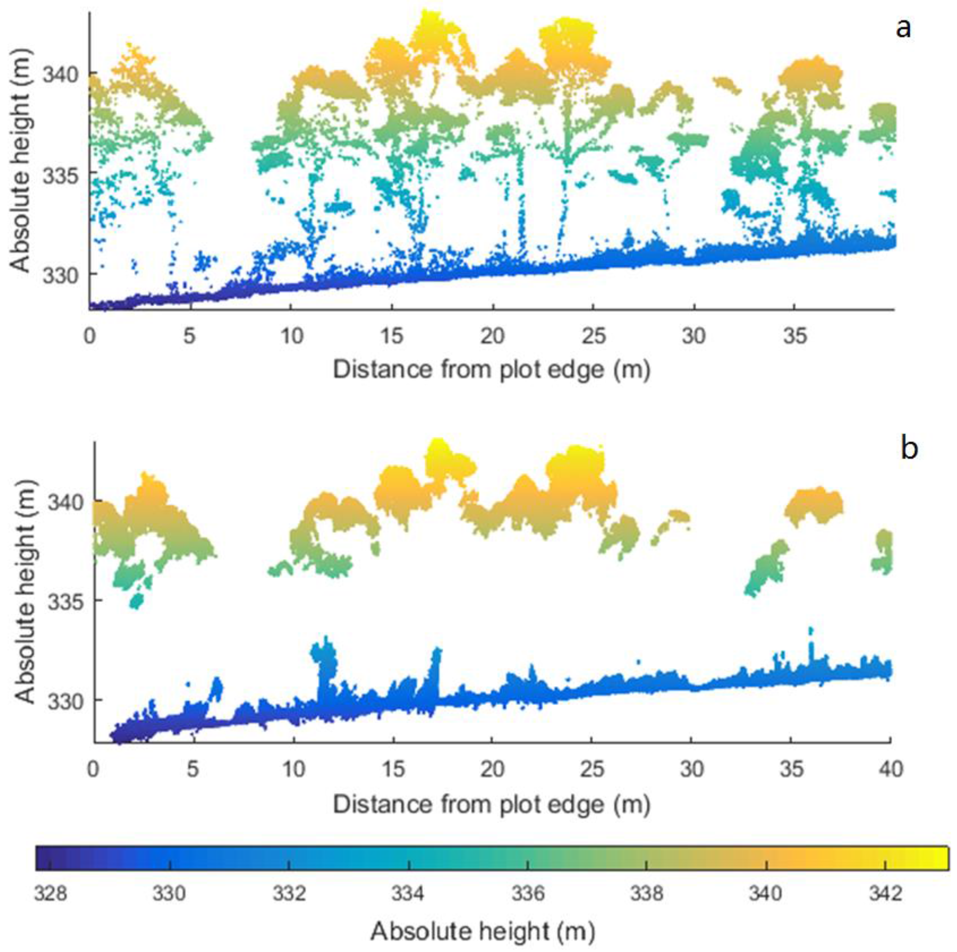
3.1. Point Cloud Properties

Figure 3a,b show examples of the point clouds produced from ALS and SfM approaches, respectively. The total processing time to create the dense point cloud from 425 RGB images was 24 h and resulted in a point cloud containing 89 million points, 85 million of which fell within the study area. The total processing time to produce a georeferenced point cloud from the ALS data took 1.5 h (0.5 h CPU time). The point density of the ALS point cloud (174 points per m²) was significantly less than the point density of the SfM point cloud (5652 points per m²). Flying four transects allowed the entire plot to be easily captured in both the ALS and SfM point clouds.

Unidentifiable ground control targets, present in both the ALS (10 identifiable targets) and SfM point clouds (14 identifiable targets), were placed too close to the edge or underneath dense canopy cover. The SfM and ALS point clouds were found to have similar horizontal and vertical accuracies when compared to the identifiable ground control targets (

Table 1. Properties of the point clouds produced from RGB imagery (SfM) and an airborne laser scanner (ALS) onboard the same UAV platform: the point cloud generation time, the number of observed Ground Control Points (GCPs), the point density, and the georeferencing accuracy (RMSE, root mean square error, SD, standard deviation).

Data Set	Point Density	GCPs	Horizontal Direction		Vertical Direction
			RMSEp (m)	SD	RMSE (m)	SD
ALS	174 pts/m2	10	0.42	0.33	0.17	0.18
SfM	5652 pts/m2	14	0.40	0.12	0.14	0.14

). The SfM point cloud produced a bias to the South-East direction, indicated by high RMSEp with a low standard deviation (SD), whereas the horizontal georeferencing error in the ALS point cloud was distributed randomly. To obtain a reliable GPS measurement accuracy, all ground control points were located in areas of low canopy cover. Hence, the georeferencing accuracy presented in Table 1 does not include the undercanopy areas.

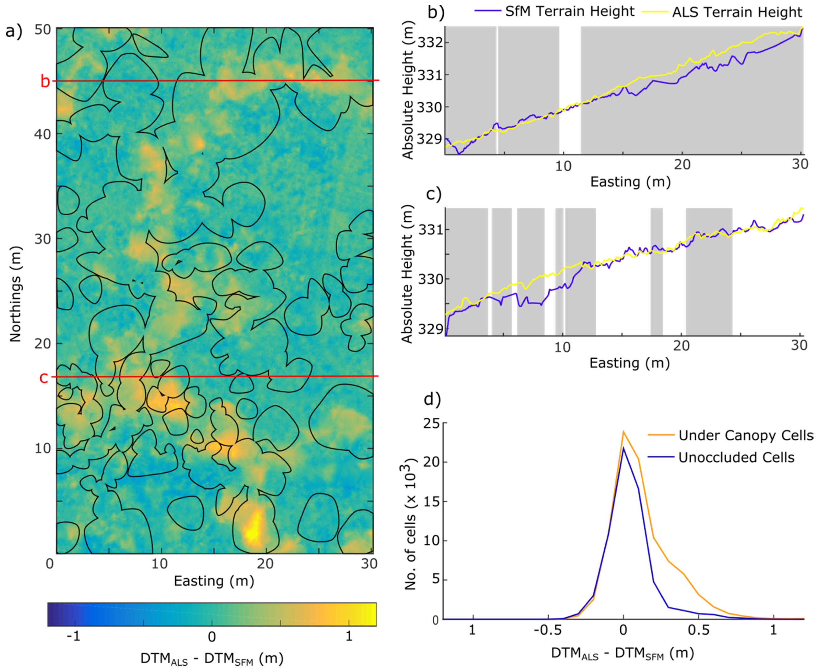
3.2. Terrain Extraction

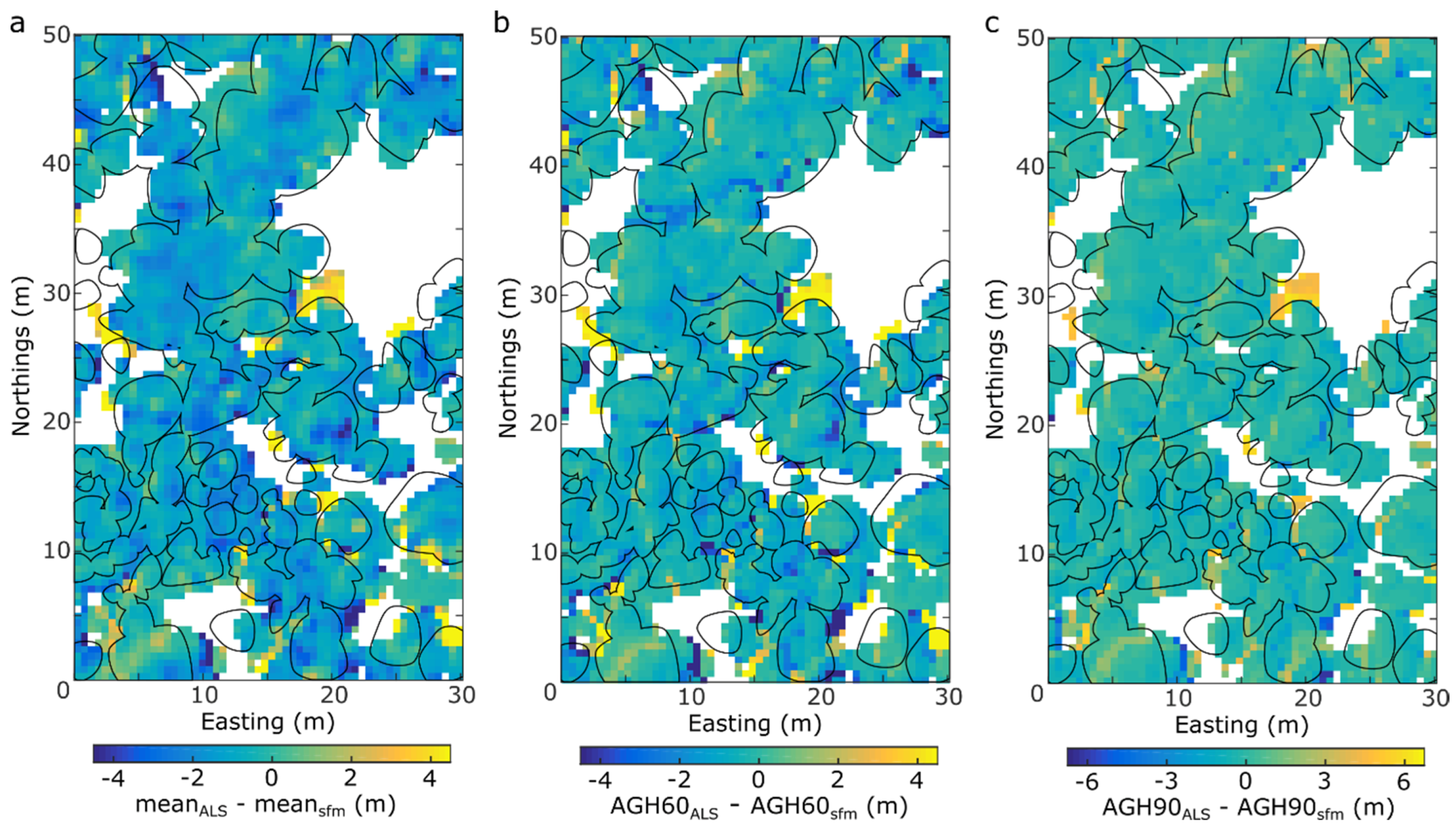
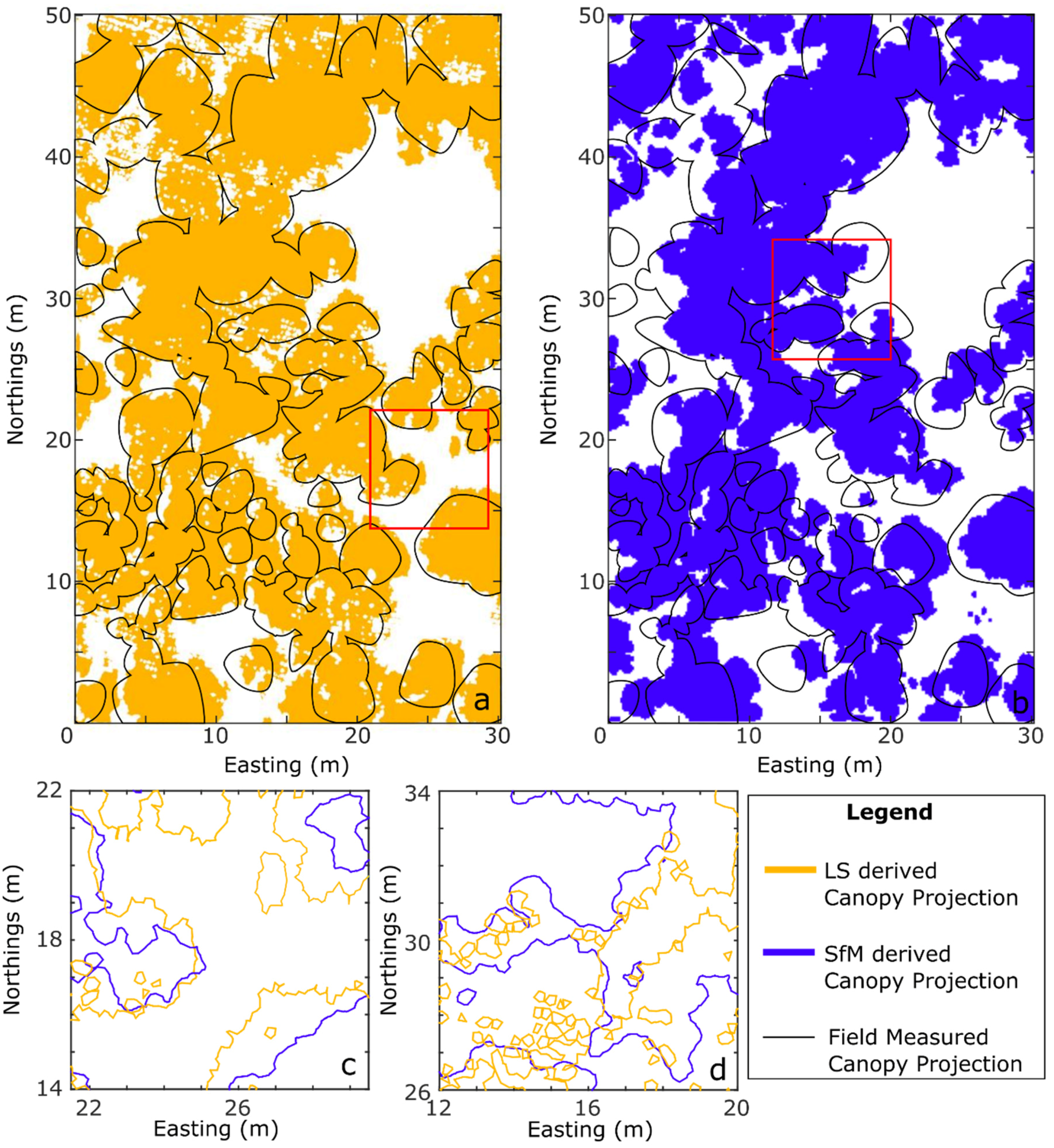
The DTM provides the ground surface, from which canopy height and vertical profiles are calculated. The accurate representation of the terrain is, therefore, crucial in characterising the 3D structure of vegetation. Overall DTM_SfM and DTM_ALS provided similar representation of the terrain across the entire plot, with a mean difference (MD) of 0.09 m. As shown in Figure 4, the largest differences in the terrain representation provided by the two methods occurred in areas covered by tree canopy, with MD of 0.12 m for cells within field measured crown projections (n = 88,185) and 0.05 m for all other cells (n = 63,921). In these under canopy areas, the terrain was not adequately sampled in the SfM point cloud, with on average only 0.5 ground points per m² extracted by the Lastools algorithm. Furthermore, the SfM algorithm appeared to significantly underestimate the terrain height at 3D points generated under the tree canopy. This likely originates from poor image geometry, due to the terrain being occuluded by forest canopy at most viewing angles. Using multiple transects with a relatively high overlap allowed the laser scanner to penetrate through small gaps in the canopy. Therefore, it produced a more even distribution of ground points throughout the plot, with an average 2 ground points per m² being recorded in areas under canopy cover. The inaccurate interpolation of ground points caused by both uncertain point locations and low density in areas of high canopy cover for DTM_SfM are most likely the cause of the large deviations between the two DTMs (under canopy absolute differences >0.5 m in some areas).

3.3. Canopy Cover

The ALS predicted a higher canopy cover across the study plot (63%) than the SfM point cloud (50%). The lower canopy cover produced by SfM results from a lack of points captured at the edge of the canopy. The field-measured crown projections, assessing a vertical canopy cover of approximately 59%, are suggesting that SfM is not capturing the vegetation cover accurately, especially towards the edge of the plot (less available images) and in locations with lower canopy layers. Due to the visual occlusion caused by higher canopy parts, features in these lower canopy layers are less likely to be captured from multiple viewing angles. Additionally, detection of reliable image features in areas of shadow is in some instances difficult. This difficulty arises due to the large brightness range between shadows and sunlit areas such as the top of the canopy and the properties and settings of the camera resulting in insufficient image contrast in areas of shadow. These effects, which could be to some extent mitigated by using a camera with a greater digital dynamic range, have also resulted in absence of a small number of understorey trees in the SfM-measured map (Figure 5b). As stated in Wallace [28], the inconsistent point density of the ALS point cloud and the use of a single alpha value is likely resulting in an under- and/or over-estimation of canopy cover in some regions (see the top left of Figure 4a for an example of underestimation). For example, the low point density in the North-Western corner of the plot has resulted in an unnatural striping pattern in the canopy cover map (Figure 5a), whereas consistent density of the SfM point cloud has resulted in a smooth representation of the canopy projection at this location (Figure 5b).

3.4. Vertical Canopy Profile

Comparison of the ALS and SfM point cloud vertical profiles suggests that SfM does not capture the foliage distribution of the middle canopy layers (Figure 6). This results in an increase in AGH percentiles between the 10th (5.45 m for ALS and 7.49 m for SfM) and the 80th percentile (10.89 m for ALS and 11.39 m for SfM). No statistically significant correlation was found between the difference in AGH percentiles estimated for a cell and the ALS or SfM canopy cover percentage estimate for that cell. Examination of the spatial distribution of differences in these statistics shows the largest differences (up to 6 m in AGH90, for example) at the edges of individual tree crowns (Figure 7). Differences found in these areas, where the SfM percentiles are lower than the ALS counterpart, result from incomplete horizontal capture of the canopy in the SfM dataset (demonstrated previously in the canopy cover maps). The lower ALS percentile values (compared to the SfM percentiles) high in the canopy result from a more complete distribution of ALS points across the vertical stratification of vegetation. Significant differences between the mean AGH of both methods are also observed towards the middle of high canopy cover areas in Figure 7b. These differences suggest that mean differences up to 3 m can occur in areas of dense canopy cover.

3.5. Individual Tree Architectural Features

The ALS and SfM datasets both contained sufficient spatial detail on the upper canopy to positively identify 122 (ALS) and 112 (SfM) tree top locations from 136 measured trees. In both datasets, trees of similar height to neighbouring trees and with highly overlapping crowns could not be positively identified. The ALS data additionally allowed for tree height to be manually digitised (as the highest point in a tree segment) for a larger number of suppressed trees that were not identifiable from the SfM point cloud. Secondly, the ALS data set also provided more sub-canopy information. This allowed a greater number of stem locations to be manually digitised (based on points occurring 1.3 m above the ground) from the ALS data (52 stems), in comparison to the SfM data (24 stems). Yet, in the both cases, the number of identified stems represents only a small proportion of the total stems within the plot.

Although both datasets showed a generally good agreement of the stem locations with the field measurements, ALS measurements were slightly better (RMSEp of 0.59 m for ALS and 1.04 m for SfM). Similarly, a stronger correlation was found between field-measured and point cloud measured tree height for ALS than for SfM (r² of 0.84 for ALS and 0.68 for SfM) (Figure 8). The ALS prediction of tree height resulted in an RMSE of 0.92 m and SfM prediction in 1.30 m, respectively. The bias of 0.34 m for ALS and 0.61 m for SfM suggests that the tree height determined by both methods was typically overestimated in comparison to the field-measured values. This positive bias may result from a number of factors, including (i) an underestimation of terrain height in both the ALS and SfM point clouds caused by overly strong ground point filtering, (ii) inaccuracies or bias in field tree height measurements caused by difficulties in determining the top of broad leaf species, and (iii) the sloping terrain.

3.6. Synthesis and Discussion of Results

This study has demonstrated the ability of point clouds captured with ALS and SfM techniques on-board a mini-UAV to estimate various structural properties of a native Australian forest stand. Both methods provided similar characterisation of the stand terrain (mean difference of 0.09 m) and of individual tree height (RMSE of 0.92 m for ALS and 1.30 m for SfM). Both techniques produced significantly higher point densities than seen in datasets captured with a similar technology on-board large manned aircraft [31]. It is also likely that the rapid development of sensor technology and application of novel analysis methods on data captured from mini-UAVs would allow for description of other forest properties that were not examined in this study, as for instance the horizontal spatial pattern, canopy base height [20], or the above ground biomass [14].

The two methods used in this paper required similar data collection effort. Both systems have also been shown capable of accurate direct data georeferencing when flown at a height of 30 m above the ground (horizontal RMSEp of 0.42 m for ALS and 0.40 m for SfM). Increased flying height is likely to cause decreases in the accuracy of the georeferencing system as outlined in Wallace et al. [32]. Given a likely use of UAVs for monitoring of vegetation dynamics [33], accurate direct georeferencing is an important processing step [13] that allows collection of accurate data in inaccessible forested terrain, where distribution and location of GCPs is often difficult. It is important to note that accurate timing of the instant photographic exposure and laser pulse is essential for obtaining the 3D georeferencing accuracy achieved in this paper. This requirement makes the design and operation of the two mapping systems similarly complex. Processing the RGB photographs to produce a dense SfM point cloud required more computational power and processing time than producing an ALS point cloud over the same study area.

The survey in this study was conceptually designed to achieve a gap-free ALS dataset. The SfM survey of four flight transects consequently produced a dense set of imagery that resulted in a very high overlap between individual RGB photos (>90%). Even with such high overlap, the SfM point cloud provided a less complete description of the vertical profile of the vegetation elements in comparison to the ALS dataset. Contrary to White et al. [22], who found an increase in the canopy cover area derived from an SfM point cloud acquired from a large piloted airplane, the UAV SfM point cloud in our study has underestimated the total canopy area in comparison to both the ALS dataset and field observations. It is likely that capturing photography along multiple flight lines that are perpendicular to the apparent flight path (i.e., a grid pattern flight path) would result in an increase of information at the crown edges. This informational increase could consequently allow a better estimate of the canopy boundaries. It is, however, unlikely to capture more information on the vertical stratification of vegetation elements located towards the centre of tree canopies and groups of trees.

In this study, we did not find any direct evidence revealing a relationship between accuracy of canopy cover estimated using ALS and differences seen in SfM and ALS point distributions. It is, however, expected that occlusion caused by dense canopy cover plays, along with a number of other factors, a role in determining this difference. For instance, the penetration ability of the laser scanner at the edge of an individual tree crown (determined by a complex relationship between vegetation configuration and laser properties [34]) is greater than towards the centre of a tree, which explains some differences observed between the SfM and ALS approaches. ALS point clouds have been previously shown to produce a high correlation between the vertical point distribution and the vertical stratification of vegetation elements [29]. As such, better canopy penetration of ALS over SfM (Figure 2) presents a significant advantage in case of a complex forest establishment.

Although ALS provides an estimate of captured photon intensity, an unfeasible number of variables would need to be resolved to determine the spectral contribution of vegetation reflectance to the acquired ALS signal. Thus, the UAV-based ALS system as presented in this study can only be used to determine the geometric/architectural properties of forest canopies. Although not being explored in this study, the spectral component of the SfM point cloud might represent an additional useful source of information for estimating other non-structural properties of the canopy. For instance, Dandois and Ellis [14] have demonstrated that spectral information captured from a UAV is able to track changes in canopy relative greenness. Additionally, Wulder et al. [35] and Getzin et al. [36] have shown that spectral channels of aerial photography can be used to discriminate some plant species, to separate woody from leafy vegetation, as well as to assess certain symptoms of the vegetation health decline.

Our results indicate that both ALS and SfM can be used to measure forest structure. The choice of which technology should be preferentially used in future forest research and applications will depend on the available budget, the properties of the study area and questions being asked. Previous studies have suggested that the SfM technique is, due to the wider field of view, able to provide greater spatial coverage than ALS [22]. In this study, we demonstrated that SfM can be used as a standalone sensing technology capable of capturing structural information in a relatively sparse forest, but it failed to measure the terrain altitude in areas of dense canopy cover. This finding, noticed also by Dandois and Ellis [14], suggests that use of SfM over increasingly denser forest canopies requires an alternative source of terrain information. UAV-based ALS, on the other hand, produced an even distribution of terrain-representing points. As such, it provides a standalone tool for measuring structure in a greater range of forest complexities. Besides, it is likely that advancements in miniaturisation of ALS technology will soon extend its capabilities in monitoring the vertical structure of forests beyond recent achievements.

Finally, this study has also demonstrated that laser scanning data and visible RGB photography can be collected simultaneously even from a single mini-UAV platform. Integrating both approaches in a single low-cost small-size airborne carrier opens up new possibilities in capturing and fusing information rich datasets that can consist of 3D structural properties together with spectral characteristics. As shown with large airborne remote sensing flying observatories [37], a mini-UAV platform combining ALS with a multispectral or hyperspectral sensor, such as presented in [38], would certainly increase capability and attractiveness of UAV remote sensing for monitoring of forested environments.

4. Conclusions

This study demonstrates that two 3D point cloud techniques, Structure-from-Motion (SfM) and airborne laser scanning (ALS), deployed on-board a mini-unmanned aerial vehicle (mini-UAV) are capable of detailed 3D mapping of forested landscape features. The two techniques have been shown to have similar operational requirements and both are capable of providing an accurate representation of the upper forest canopy layer (tree height RMSE of 0.92 m for ALS and 1.30 m for SfM). Furthermore, both technologies provided a high-resolution indication of the properties of the terrain and low-lying vegetation layers in sparse areas of the canopy. However, ALS was able to better penetrate the upper canopy, and consequently provide a more complete estimate of the vertical distribution of vegetation. SfM lacked the ability to penetrate dense canopy parts, which resulted in a poor definition of the mid- and under-storey. This study also demonstrated that simultaneous capture and direct georeferencing of both ALS and SfM data from a small-size mini-UAV platform is operationally achievable. As such, it presents a unique opportunity to capture on-demand high-resolution 3D information of various natural as well as intensively managed landscapes.

References

1. McElhinny, C.; Gibbons, P.; Brack, C.; Bauhus, J. Forest and woodland stand structural complexity: Its definition and measurement. For. Ecol. Manag. 2005, 218, 1–24. [Google Scholar] [CrossRef]
2. Lindenmayer, D.B.; Margules, C.R.; Botkin, D.B.; Biology, C.; Aug, N. Indicators of Biodiversity for Ecologically Sustainable Forest Management. Conserv. Biol. 2007, 14, 941–950. [Google Scholar] [CrossRef]
3. Keith, H.; Mackey, B.G.; Lindenmayer, D.B. Re-evaluation of forest biomass carbon stocks and lessons from the world’s most carbon-dense forests. Proc. Natl. Acad. Sci. USA 2009, 106, 11635–11640. [Google Scholar] [CrossRef] [PubMed]
4. Gómez, C.; Wulder, M.A.; Montes, F.; Delgado, J.A. Modeling forest structural parameters in the mediterranean pines of central Spain using QuickBird-2 imagery and classification and regression tree analysis (CART). Remote Sens. 2012, 4, 135–159. [Google Scholar] [CrossRef]
5. Kane, V.R.; North, M.P.; Lutz, J.A.; Churchill, D.J.; Roberts, S.L.; Smith, D.F.; McGaughey, R.J.; Kane, J.T.; Brooks, M.L. Assessing fire effects on forest spatial structure using a fusion of Landsat and airborne LiDAR data in Yosemite National Park. Remote Sens. Environ. 2013, 151, 89–101. [Google Scholar] [CrossRef]
6. Zellweger, F.; Braunisch, V.; Baltensweiler, A.; Bollmann, K. Remotely sensed forest structural complexity predicts multi species occurrence at the landscape scale. For. Ecol. Manag. 2013, 307, 303–312. [Google Scholar] [CrossRef]
7. Hill, A.; Breschan, J.; Mandallaz, D. Accuracy Assessment of Timber Volume Maps Using Forest Inventory Data and LiDAR Canopy Height Models. Forests 2014, 5, 2253–2275. [Google Scholar] [CrossRef]
8. St-Onge, B.; Audet, F.-A.; Bégin, J. Characterizing the Height Structure and Composition of a Boreal Forest Using an Individual Tree Crown Approach Applied to Photogrammetric Point Clouds. Forests 2015, 6, 3899–3922. [Google Scholar] [CrossRef]
9. Ota, T.; Ogawa, M.; Shimizu, K.; Kajisa, T.; Mizoue, N.; Yoshida, S.; Takao, G.; Hirata, Y.; Furuya, N.; Sano, T.; et al. Aboveground Biomass Estimation Using Structure from Motion Approach with Aerial Photographs in a Seasonal Tropical Forest. Forests 2015, 6, 3882–3898. [Google Scholar] [CrossRef]
10. Matese, A.; Toscano, P.; Di Gennaro, S.F.; Genesio, L.; Vaccari, F.P.; Primicerio, J.; Belli, C.; Zaldei, A.; Bianconi, R.; Gioli, B. Intercomparison of UAV, Aircraft and Satellite Remote Sensing Platforms for Precision Viticulture. Remote Sens. 2015, 7, 2971–2990. [Google Scholar] [CrossRef]
11. Zarco-Tejada, P.J.; Diaz-Varela, R.; Angileri, V.; Loudjani, P. Tree height quantification using very high resolution imagery acquired from an unmanned aerial vehicle (UAV) and automatic 3D photo-reconstruction methods. Eur. J. Agron. 2014, 55, 89–99. [Google Scholar] [CrossRef]
12. Lucieer, A.; Turner, D.; King, D.; Robinson, S. Using an unmanned aerial vehicle (UAV) to capture micro-topography of antarctic moss beds. Int. J. Appl. Earth Obs. Geoinf. 2014, 27, 53–62. [Google Scholar] [CrossRef]
13. Turner, D.; Lucieer, A.; Wallace, L. Direct georeferencing of ultrahigh-resolution UAV imagery. IEEE Trans. Geosci. Remote Sens. 2014, 52, 2738–2745. [Google Scholar] [CrossRef]
14. Dandois, J.P.; Ellis, E.C. High spatial resolution three-dimensional mapping of vegetation spectral dynamics using computer vision. Remote Sens. Environ. 2013, 136, 259–276. [Google Scholar] [CrossRef]
15. Jaakkola, A.; Hyyppä, J.; Kukko, A.; Yu, X.; Kaartinen, H.; Lehtomäki, M.; Lin, Y. A low-cost multi-sensoral mobile mapping system and its feasibility for tree measurements. ISPRS J. Photogramm. Remote Sens. 2010, 65, 514–522. [Google Scholar] [CrossRef]
16. Lisein, J.; Pierrot-Deseilligny, M.; Bonnet, S.; Lejeune, P. A Photogrammetric Workflow for the Creation of a Forest Canopy Height Model from Small Unmanned Aerial System Imagery. Forests 2013, 4, 922–944. [Google Scholar] [CrossRef]
17. Wallace, L.; Musk, R.; Lucieer, A. An assessment of the repeatability of automatic forest inventory metrics derived from UAV-borne laser scanning data. IEEE Trans. Geosci. Remote Sens. 2014, 52, 7160–7169. [Google Scholar] [CrossRef]
18. Wallace, L.; Lucieer, A.; Watson, C.; Turner, D. Development of a UAV-LiDAR system with application to forest inventory. Remote Sens. 2012, 4, 1519–1543. [Google Scholar] [CrossRef]
19. Snavely, N.; Seitz, S.M.; Szeliski, R. Modeling the world from Internet photo collections. Int. J. Comput. Vis. 2008, 80, 189–210. [Google Scholar] [CrossRef]
20. Wallace, L.; Watson, C.; Lucieer, A. Detecting pruning of individual stems using airborne laser scanning data captured from an Unmanned Aerial Vehicle. Int. J. Appl. Earth Obs. Geoinf. 2014, 30, 76–85. [Google Scholar] [CrossRef]
21. Wallace, L.; Lucieer, A.; Watson, C.S. Evaluating tree detection and segmentation routines on very high resolution UAV LiDAR data. IEEE Trans. Geosci. Remote Sens. 2014, 52, 7619–7628. [Google Scholar] [CrossRef]
22. White, J.C.; Wulder, M.A.; Vastaranta, M.; Coops, N.C.; Pitt, D.; Woods, M. The utility of image-based point clouds for forest inventory: A comparison with airborne laser scanning. Forests 2013, 4, 518–536. [Google Scholar] [CrossRef]
23. White, J.; Stepper, C.; Tompalski, P.; Coops, N.; Wulder, M. Comparing ALS and Image-Based Point Cloud Metrics and Modelled Forest Inventory Attributes in a Complex Coastal Forest Environment. Forests 2015, 6, 3704–3732. [Google Scholar] [CrossRef]
24. Penner, M.; Woods, M.; Pitt, D.A. Comparison of Airborne Laser Scanning and Image Point Cloud Derived Tree Size Class Distribution Models in Boreal Ontario. Forests 2015, 6, 4034–4054. [Google Scholar] [CrossRef]
25. Verhoeven, G. Taking Computer Vision Aloft-Archeological Three-dimensional Reconstructions from Aerial Photographs with PhotoScan. Archaeol. Prospect. 2011, 18, 67–73. [Google Scholar] [CrossRef]
26. Isenburg, M. Lastools: Converting, Filtering, Viewing, Gridding, and Compressing Lidar Data. Available online: http://www.cs.unc.edu/~isenburg/lastools/ (accessed on 4 March 2016).
27. Edelsbrunner, H.; Mücke, E.P. Three-dimensional alpha shape. ACM Trans. Graph. 1994, 13, 43–72. [Google Scholar] [CrossRef]
28. Wallace, L. Assessing the stability of canopy maps produced from UAV-LiDAR data. In Proceedings of the 2013 IEEE International Geoscience and Remote Sensing Symposium (IGARSS), Melbourne, Victoria, 21–26 July 2013; pp. 3879–3882.
29. Chasmer, L.; Hopkinson, C.; Treitz, P. Investigating laser pulse penetration through a conifer canopy by integrating airborne and terrestrial lidar. Can. J. Remote Sens. 2006, 32, 116–125. [Google Scholar] [CrossRef]
30. Kaartinen, H.; Hyyppä, J.; Yu, X.; Vastaranta, M.; Hyyppä, H.; Kukko, A.; Holopainen, M.; Heipke, C.; Hirschmugl, M.; Morsdorf, F.; et al. An international comparison of individual tree detection and extraction using airborne laser scanning. Remote Sens. 2012, 4, 950–974. [Google Scholar] [CrossRef] [Green Version]
31. McRoberts, R.E.; Næsset, E.; Gobakken, T.; Bollandsås, O.M. Indirect and direct estimation of forest biomass change using forest inventory and airborne laser scanning data. Remote Sens. Environ. 2015, 164, 36–42. [Google Scholar] [CrossRef]
32. Wallace, L.; Lucieer, A.; Turner, D.; Watson, C. Error assessment and mitigation for hyper-temporal UAV-borne LiDAR surveys of forest inventory. In Proceedings of the SilviLaser, Hobart, Tasmania, 16–19 October 2011.
33. Anderson, K.; Gaston, K.J. Lightweight unmanned aerial vehicles will revolutionize spatial ecology. Front. Ecol. Environ. 2013, 11, 138–146. [Google Scholar] [CrossRef]
34. Disney, M.I.; Kalogirou, V.; Lewis, P.; Prieto-Blanco, A.; Hancock, S.; Pfeifer, M. Simulating the impact of discrete-return lidar system and survey characteristics over young conifer and broadleaf forests. Remote Sens. Environ. 2010, 114, 1546–1560. [Google Scholar] [CrossRef]
35. Wulder, M.A.; White, J.C.; Coggins, S.; Ortlepp, S.M.; Coops, N.C.; Heath, J.; Mora, B. Digital high spatial resolution aerial imagery to support forest health monitoring: The mountain pine beetle context. J. Appl. Remote Sens. 2012, 6, 062527. [Google Scholar]
36. Getzin, S.; Wiegand, K.; Schöning, I. Assessing biodiversity in forests using very high-resolution images and unmanned aerial vehicles. Methods Ecol. Evol. 2012, 3, 397–404. [Google Scholar] [CrossRef]
37. Asner, G.P.; Knapp, D.E.; Kennedy-Bowdoin, T.; Jones, M.O.; Martin, R.E.; Boardman, J.; Field, C.B. Carnegie Airborne Observatory: In-flight fusion of hyperspectral imaging and waveform light detection and ranging for three-dimensional studies of ecosystems. J. Appl. Remote Sens. 2007, 1, 013536. [Google Scholar] [CrossRef]
38. Lucieer, A.; Malenovsky, Z.; Veness, T.; Wallace, L. HyperUAS-Imaging Spectroscopy from a Multirotor Unmanned Aircraft System. J. F. Robot. 2014, 4, 571–590. [Google Scholar] [CrossRef]
Figure 1. The small-UAV platform used to collect both airborne RGB photography and laser scanning data.
Forests 07 00062 g001
Figure 2. Field-measured crown projections within the study plot (left) and a photo looking into the plot from the South-East corner (right).
Forests 07 00062 g002
Figure 3. (a) Side-view of a transect through the study plot generated from the point cloud of the ALS system and (b) the same produced using RGB photography and the SfM algorithm.
Forests 07 00062 g003
Figure 4. (a) Spatial distribution, (b) and (c) transects (indicated in a) extracted across DTMSfM and DTMALS, and (d) histogram of the height difference between DTMSfM and DTMALS. The black polygons in (a) represent the silhouettes of field-measured horizontal crown projections, and the shaded areas in (b) and (c) represent generated canopy cover.
Forests 07 00062 g004
Figure 5. The alpha shape canopy cover maps produced from the (a) ALS (orange shaded area) and (b) SfM (blue shaded area) point clouds. The black lines represent the silhouettes of field-measured horizontal crown projections; Direct comparisons of the ALS and SfM techniques in (c) and (d) showing two detailed subsets outlined by red squares in a and b, respectively.
Forests 07 00062 g005
Figure 6. Above ground height distribution of points (>1.5 m above the ground) in the ALS all returns, ALS first returns only, and SfM point clouds captured within the entire plot boundary.
Forests 07 00062 g006
Figure 7. Spatial difference in the (a) mean AGH, (b) 60th above ground height percentiles (c) 90th above ground height percentiles as derived from ALS and SfM datasets. The black lines represent the silhouettes of field-measured horizontal crown projections. The white (no data) cells have minimal or no information above a height of 1.3 m.
Forests 07 00062 g007
Figure 8. (a) ALS determined tree height compared to field-measured tree height; (b) SfM determined tree height compared to field-measured tree height; and (c) ALS height against SfM height. The dashed line represents the 1:1 line and the solid line represents the fitted linear function.
Forests 07 00062 g008