Application of Wildfire Risk Assessment Results to Wildfire Response Planning in the Southern Sierra Nevada, California, USA

Abstract

How wildfires are managed is a key determinant of long-term socioecological resiliency and the ability to live with fire. Safe and effective response to fire requires effective pre-fire planning, which is the main focus of this paper. We review general principles of effective federal fire management planning in the U.S., and introduce a framework for incident response planning consistent with these principles. We contextualize this framework in relation to a wildland fire management continuum based on federal fire management policy in the U.S. The framework leverages recent advancements in spatial wildfire risk assessment—notably the joint concepts of in situ risk and source risk—and integrates assessment results with additional geospatial information to develop and map strategic response zones. We operationalize this framework in a geographic information system (GIS) environment based on landscape attributes relevant to fire operations, and define Potential wildland fire Operational Delineations (PODs) as the spatial unit of analysis for strategic response. Using results from a recent risk assessment performed on several National Forests in the Southern Sierra Nevada area of California, USA, we illustrate how POD-level summaries of risk metrics can reduce uncertainty surrounding potential losses and benefits given large fire occurrence, and lend themselves naturally to design of fire and fuel management strategies. To conclude we identify gaps, limitations, and uncertainties, and prioritize future work to support safe and effective incident response.

1. Introduction

In the western U.S. and elsewhere, new paradigms are emerging that recognize a need to deemphasize fire exclusion, expand application of prescribed and managed natural fire, and foster resilience and adaptation to fire [1,2,3,4]. The National Cohesive Wildland Fire Management Strategy in the U.S. focuses on making meaningful progress towards attainment of resilient landscapes, fire adapted communities, and safe and effective response to fire [5]. Our focus here is the goal of safe and effective response to fire, and is based on the premise that how fires are managed—not just how landscapes are managed and communities respond before and after fires occur—is a key determinant of long-term socioecological resiliency and the ability to “live with fire” [6,7,8].

Improving the safety and effectiveness of response to fire requires a multi-faceted approach. At the tactical and operational level enhancing firefighter safety remains a priority, as is the evaluation of suppression resource use and effectiveness (e.g., [9,10]). From a broader organizational perspective, improving response effectiveness requires ensuring that fire management objectives are consistent with land and resource objectives, and that implemented fire management strategies are likely to move landscapes toward desired conditions. Effective response therefore requires the existence of clear, consistent, risk-informed fire management objectives as well as guidance for how to achieve those objectives, i.e., effective response requires effective pre-fire planning (3).

Meyer et al. [11] comprehensively review principles of effective federal fire management planning in the U.S. as they relate to contemporary policy; here we generalize and distill some essential features to motivate the current study. First, the plans must be spatially explicit—this includes mapping highly valued resources and assets (HVRAs) that may be impacted by fire, as well as landscape attributes (e.g., roads and ridgetops) relevant to fire operations. Second, plans must be developed using the best available science and information. Third, plans must be flexible and adaptive in order to be responsive to changing conditions. Investing in pre-fire planning can ultimately help alleviate some of the uncertainties and the time pressures that characterize the incident response decision environment [12].

In this paper we introduce a framework for incident response planning that is consistent with these principles. We leverage recently developed concepts and techniques in spatial risk assessment and integrate results with additional geospatial information to develop and map strategic response zones. In particular we focus on two alternative spatial representations of risk: in situ and source. In situ risk analysis reflects localized (i.e., raster-based) estimates of potential losses or benefits given the presence of at least one HVRA in the given location, and these estimates can be expressed conditionally or weighted by the location-specific probability of fire occurrence using stochastic fire spread modeling [13,14,15,16]. Risk source analysis by contrast focuses not on where the losses or benefits might occur, but rather where the risk might originate, estimated by determining fire-level HVRA losses and benefits and associating these aggregate impacts back to a given ignition location using a set of simulated fire perimeters [17]. A broad range of applications have used similar fire modeling approaches to quantify HVRA exposure to fire without directly modeling consequences (e.g., [18,19,20,21,22,23,24]).

There are four primary purposes to this research effort. First and foremost is to demonstrate the potential utility of a spatial fire planning framework and the guidance offered by predefined strategic response zones. Second, we illustrate how the concepts of in situ and source risk can help managers better understand potential consequences and evaluate responses to fire. Third, we outline a method to operationalize the response planning framework in a geographic information system (GIS) environment based on landscape attributes relevant to fire operations. Lastly, we identify gaps, limitations, and uncertainties, and prioritize future work to support safe and effective incident response.

2. A Spatial, Risk-Informed, Flexible Framework for Incident Response

In the U.S., current federal wildland fire management policy affords a large degree of flexibility in response to fire, ranging from aggressive suppression in order to achieve protection objectives to managing naturally ignited fires when conditions are favorable in order to achieve resource objectives. Managers may also intentionally ignite wildland fires (i.e., prescribed fires) to reduce hazard or enhance resource conditions, when conditions, regulations, and other constraints allow.

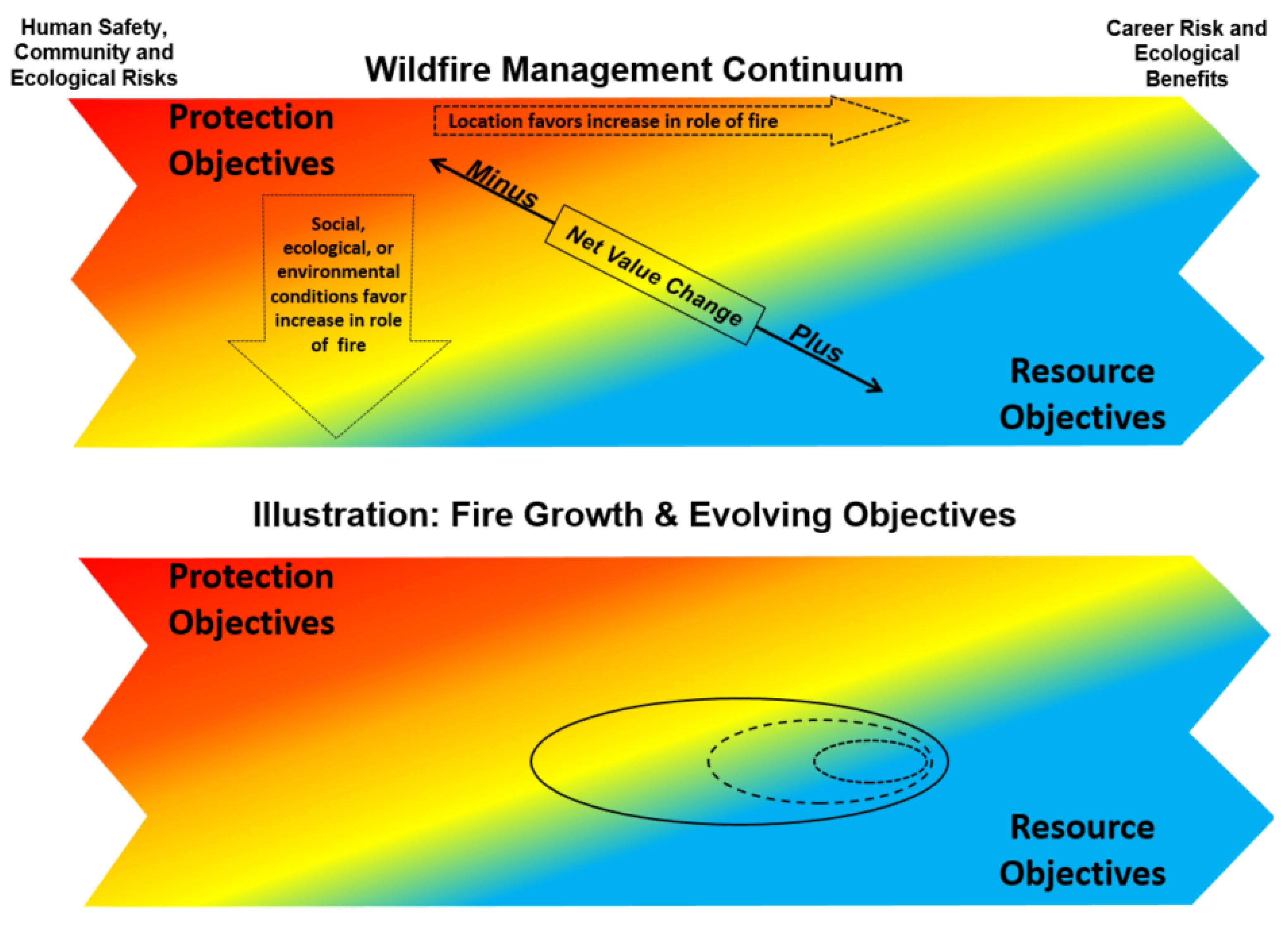
The conceptual Wildland Fire Management Continuum (Figure 1) visually depicts how a wildland fire may be concurrently managed for one or more objectives. How objectives are identified and balanced can change as the fire spreads across the landscape and as the conditions under which the fire is burning change. Objectives are affected by: changes in fuels, weather, topography; varying social understanding and tolerance; and involvement of other governmental jurisdictions having different missions and objectives. Other factors that influence response include human safety risk, ecological risk, perceived career risk (e.g., liability issues or adverse performance reviews if a fire managed for resource benefit escapes control and causes damage), management requirements, and regulations.

The basics of the Wildland Fire Management Continuum can be described according to four dimensions:

• The length (side to side) of the Continuum shows the spatial component—the location of the fire on the landscape—that affects the mix of objectives. Spatial risk assessment results directly speak to this dimension of the continuum, and the central idea is that potential losses and benefits across the landscape have been assessed up front. On the left, the location favors protection objectives, whereas on the right resources objectives are favored.
• The width (up and down) of the Continuum illustrates the different social, ecological or environmental conditions affecting the mix of objectives. This dimension allows for flexibility in response decisions considering factors not easily captured with spatial risk assessments. On the top, protection objectives prevail, whereas on the bottom resource objectives are easier to meet.
• The colors across the Continuum depict the range of objectives taking in the combination of both location and conditions. Red (upper left) represents where the combination of conditions and landscape location result in protection as the predominate objective. Blue (lower right) instead represents conditions where enhancing resource conditions is the primary objective.
• The teeth on each end of the Continuum are to show that it wraps around to form a cylinder. As an example, a fire intended to be managed exclusively for ecological purposes may escape control due to major changes in weather conditions, grow rapidly to threaten resources and assets, and management efforts would transition to aggressive suppression (e.g., the 2000 Cerro Grande Fire that began as a prescribed fire but escaped and caused significant damage to Los Alamos, New Mexico, USA).

As a conceptual model the Continuum is useful for a range of management and planning horizons, with varying degrees of change in relevant social, ecological, or environmental conditions. For example, across fire seasons, changes in air quality regulations and population growth may lead to smoke concerns limiting opportunities for increased fire, even in locations where ecological benefits would likely result. Similarly, changes in fuel conditions due to succession and disturbance may lead some locations to present greater or lesser risk. At a smaller time scale, over the course of a single fire event, social concerns such as tolerance of smoke or restricted recreational access could influence management opportunities. It is important to note that in the incident management context the location dimension becomes dynamic as the fire grows across the landscape, and as a result may be the more important factor in determining management objectives. The bottom panel of Figure 1 presents a stylized illustration of a fire growing as an ellipse. Although the fire ignited in a location suitable for resource objectives, the fire grew in the direction of an area containing resources and assets more susceptible to loss, likely leading to protection objectives dictating response strategies along the head and flanks of the fire. In reality, as a specific incident unfolds fire managers have access to tailored decision support functionality and more detailed information on risks and opportunities to help determine response objectives and actions. Thus, although the conceptual underpinnings of the Continuum have clear relevance for risk-informed and dynamic incident management, the Continuum is perhaps most useful for planning applications in advance of incidents.

Synthesizing risk assessment results according to the location dimension allows for the landscape to be zoned according to broad strategic response categories. Further on we will describe our spatial approach to zoning up the landscape. This process is not dissimilar from past practices that stated objectives and appropriate responses at the administrative fire management unit level, but with the explicit intention to create zones that are spatially logical relative to landscape attributes, fire management operations, and assessed risks, and that therefore translate more clearly to fire management objectives and response guidance. Note that a given response category may encompass a range of protection and resource objectives, and how categories are differentiated is not necessarily black and white. The aim however is not to predetermine response decisions, but rather to simplify the decision space while accounting for flexibility in response to changing conditions. The ultimate intent is to provide useful support to strategic response decisions and more broadly to fuel management and forest restoration decisions.

For proof-of-concept, below we define and describe three generalized strategic response zone categories. In practice additional categories can be created and tailored to the specific planning context, and spatial response zone boundaries can updated through time in response to changing conditions. In fact this delineation of zones lends itself to a quantifiable performance measure, the amount of area that moves between zones over time (moving from protection to restoration, for instance, would be indicative of reduced risk).

• Protect: Current conditions are such that HVRAs are at high risk of loss from wildfire. Mechanical fuel treatments would principally be used to yield desired fire behavior conducive to more effective fire suppression, or in some instances retention of desired conditions for natural resources. Prescribed burning would principally be used to maintain previously treated areas. The use of wildfire to increase ecosystem resilience and provide ecological benefits would be very limited.
• Restore: Current conditions are such that HVRAs are at moderate risk of loss from wildfire. Wildfire could be used to increase ecosystem resilience and provide ecological benefits when conditions allow. Strategically located mechanical treatments and/or prescribed burning, where feasible, may be a necessary precursor to the reintroduction of wildfire to achieve desired conditions.
• Maintain: Current conditions are such that HVRAs are at low risk of loss from wildfire, and many natural resources may benefit from fire. Due to low risk, wildfires are expected to be used as often as possible to maintain ecosystem resilience and provide ecological benefits when conditions allow. Mechanical treatments and/or prescribed burning, where feasible, are used to complement wildfire to achieve desired conditions. Aggressive suppression to keep fires as small as possible would be very limited.

3. Methods

We organize our description of methods as follows. First, we identify the study area we use to operationalize the response planning work, and describe its relevance to real-world decision support for US Forest Service land and fire management planning. Next, we describe our spatial risk assessment methods, focusing primarily on a novel stochastic fire simulation approach developed to account for the size and heterogeneity of the study area, as well as the in situ and source risk calculations. Lastly, we describe the generation of Potential wildland fire Operational Delineations (PODs) as the fundamental spatial unit of analysis for assigning response categories, and define our categorization schema.

3.1. Study Area

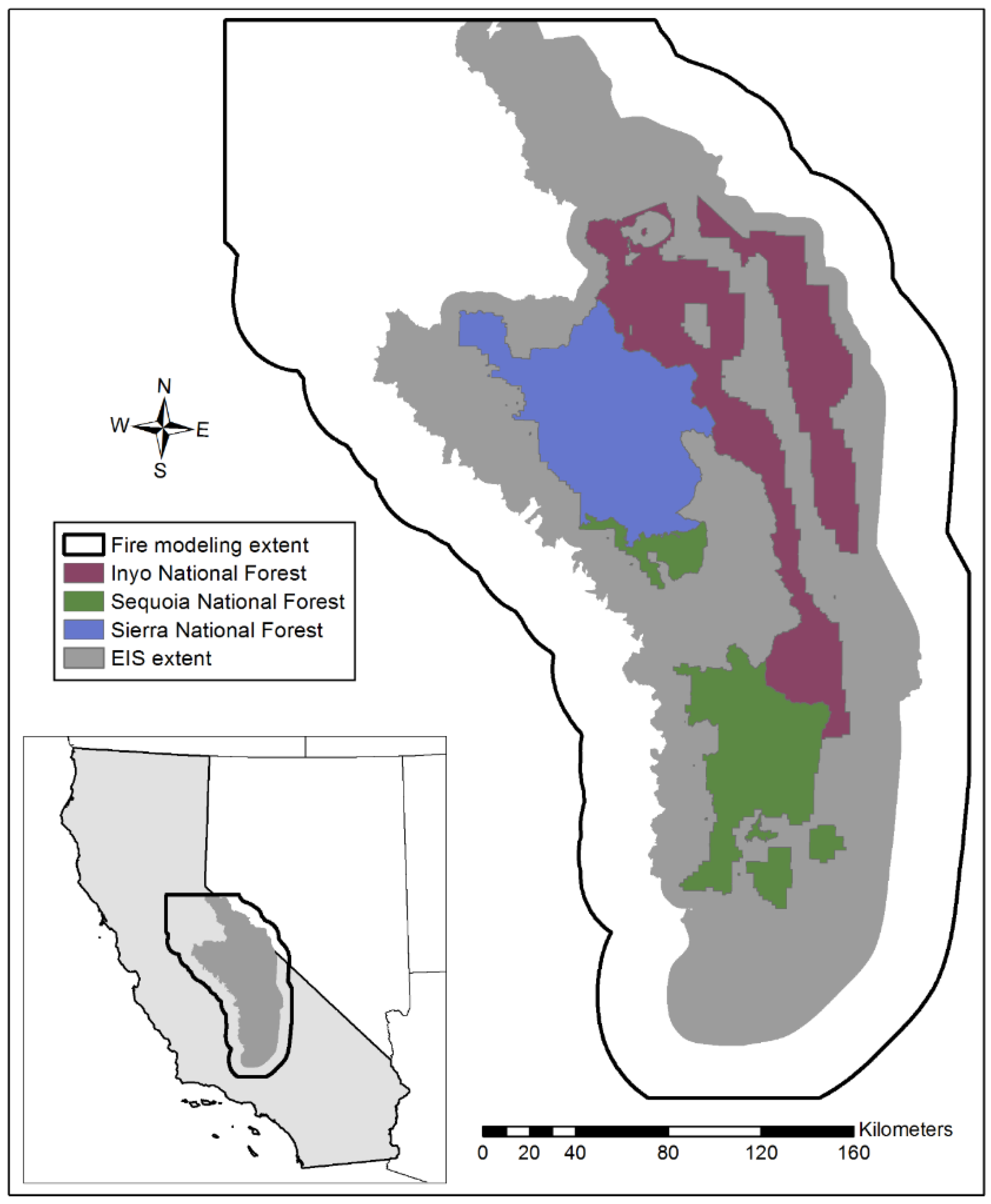
The study area encompasses the Inyo, Sequoia, and Sierra National Forests, which are located in the southern Sierra Nevada Mountains in California, USA. These three Forests are “early adopters” of the US Forest Service’s 2012 Planning Rule, and as of this writing are in the process of updating their Land and Resource Management Plans (LRMPs). Agency-wide guidance directs National Forests to spatially depict LRMPs, and the Pacific Southwest Region further directs National Forests in California to incorporate fire management wildfire risk into these plans. Guidance in LRMPs ultimately provides the basis for spatial fire plans as well as strategic fire management objectives.

Part of the plan revision process is documentation of an Environmental Impact Statement (EIS) as required by the National Environmental Policy Act (NEPA), and our study area includes the EIS extent for these three National Forests. The fire modeling extent (Figure 2) reflects a buffered area around these Forests so that valid results could be produced not only within each Forest, but also in the land area adjacent to the Forests. All HVRAs are mapped to the EIS extent. The authors, along with staff from local Forests and the Pacific Southwest Region, jointly designed and implemented the Southern Sierra Risk Assessment (SSRA) to support planning efforts. It is important to clarify that while we use many of the data, processes, and products generated as part of the SSRA, what we present here is a generalized depiction of the response planning framework and does not reflect the specifics of any NEPA-related decision processes.

3.2. Fire Occurrence Areas

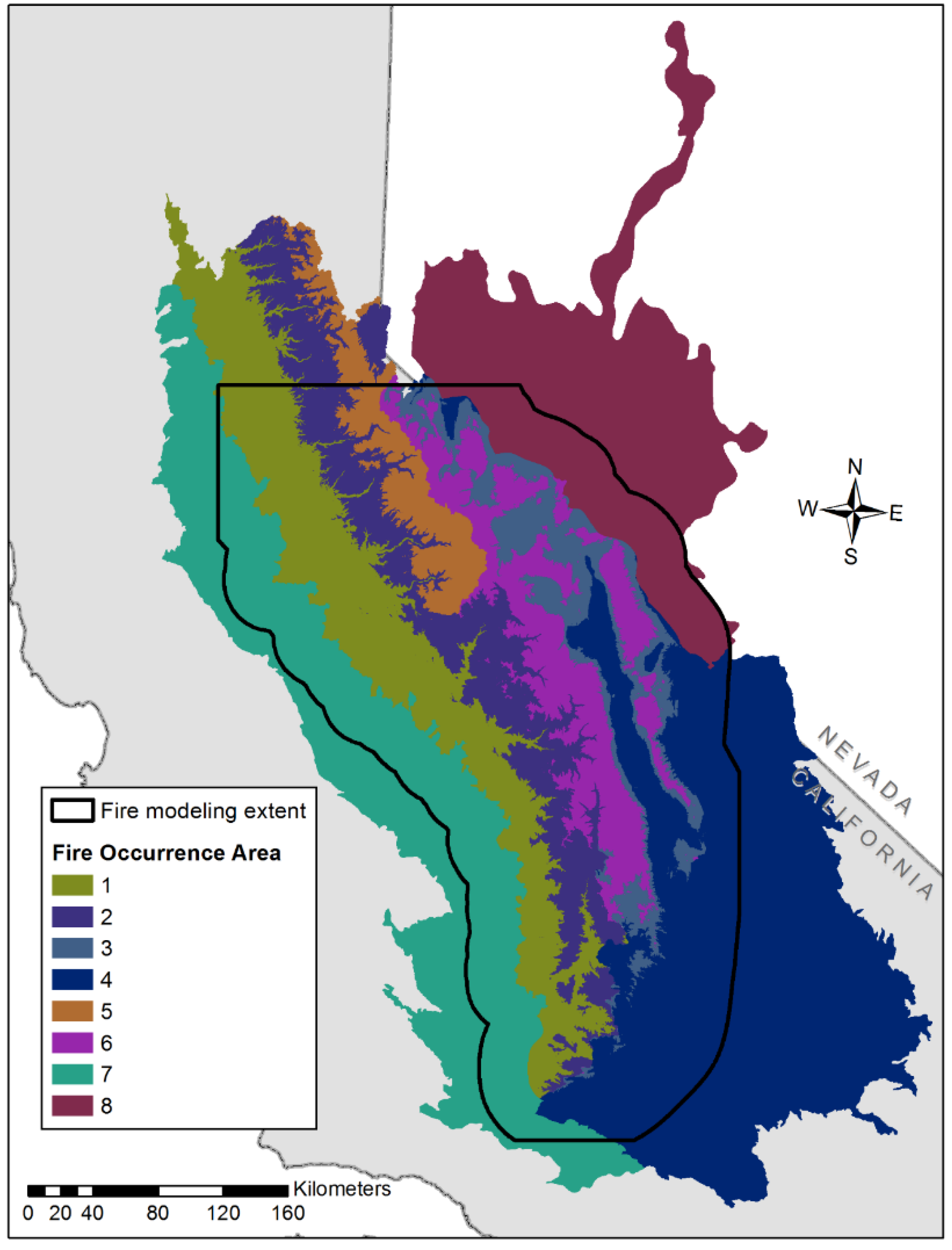
The fire modeling area for the SSRA area is a 9.7 million ha extent characterized by vegetation conditions ranging from valley-bottom grasslands in the Central Valley to alpine timber at the highest elevations, and to arid sagebrush shrubland on the lee side of the Sierra crest. Because this landscape is so large and variable, historical fire occurrence and fire weather summaries for the entire area are inadequate to characterize the variability within and among some of the distinct vegetation communities found along elevation gradients within this landscape. Therefore, we summarized historical fire occurrence for eight different fire occurrence areas (FOAs) within the SSRA greater landscape. The boundaries for these areas are based on elevation-based ecozones, aggregated where appropriate for fire modeling purposes. The resulting FOAs are mapped in Figure 3 and their land-area extent summarized in

Table 1. Summary of total area, fire-modeling area, and Remote Automated Weather Station (RAWS) station used in each of the eight fire occurrence areas (FOAs) used in the Southern Sierra Risk Assessment.

FOA	Total Hectares	Fire Modeling Hectares	RAWS Station Used
1	2,157,931	1,756,236	Trimmer
2	1,636,274	1,255,834	Mount Elizabeth
3	816,730	813,484	Oak Creek
4	4,422,598	1,917,912	Oak Creek
5	583,919	418,494	Blackrock
6	1,194,651	1,191,764	Blackrock
7	3,250,189	1,662,750	Trimmer
8	2,605,756	706,760	Oak Creek

.

3.3. Historical Fire Occurrence and Weather Data

We used the Short [25] Fire Occurrence Database (FOD) as the foundation for summarizing fire occurrence within each of the eight FOAs described in the previous section. For each FOA, records were selected from the FOD based on the start location of each wildfire. This process produced eight tabular FODs. Though we retained all attributes of the original FOD, the main attributes of interest are the start location, start date, final fire size, and cause class (human-caused vs. natural). Specifically we queried the FOD for information on “large fires”, defined here as greater or equal to 100 ha.

These tabular datasets were summarized to estimate two main contemporary, historical large-fire occurrence measures for each FOA: mean annual number of large fires, and mean annual large-fire area burned. We tabulated these measures across the entire FOA, including portions beyond the fire modeling landscape extent, and normalized the annual occurrence rates to a per-million-acres basis to permit comparison of wildfire occurrence across FOAs of different sizes.

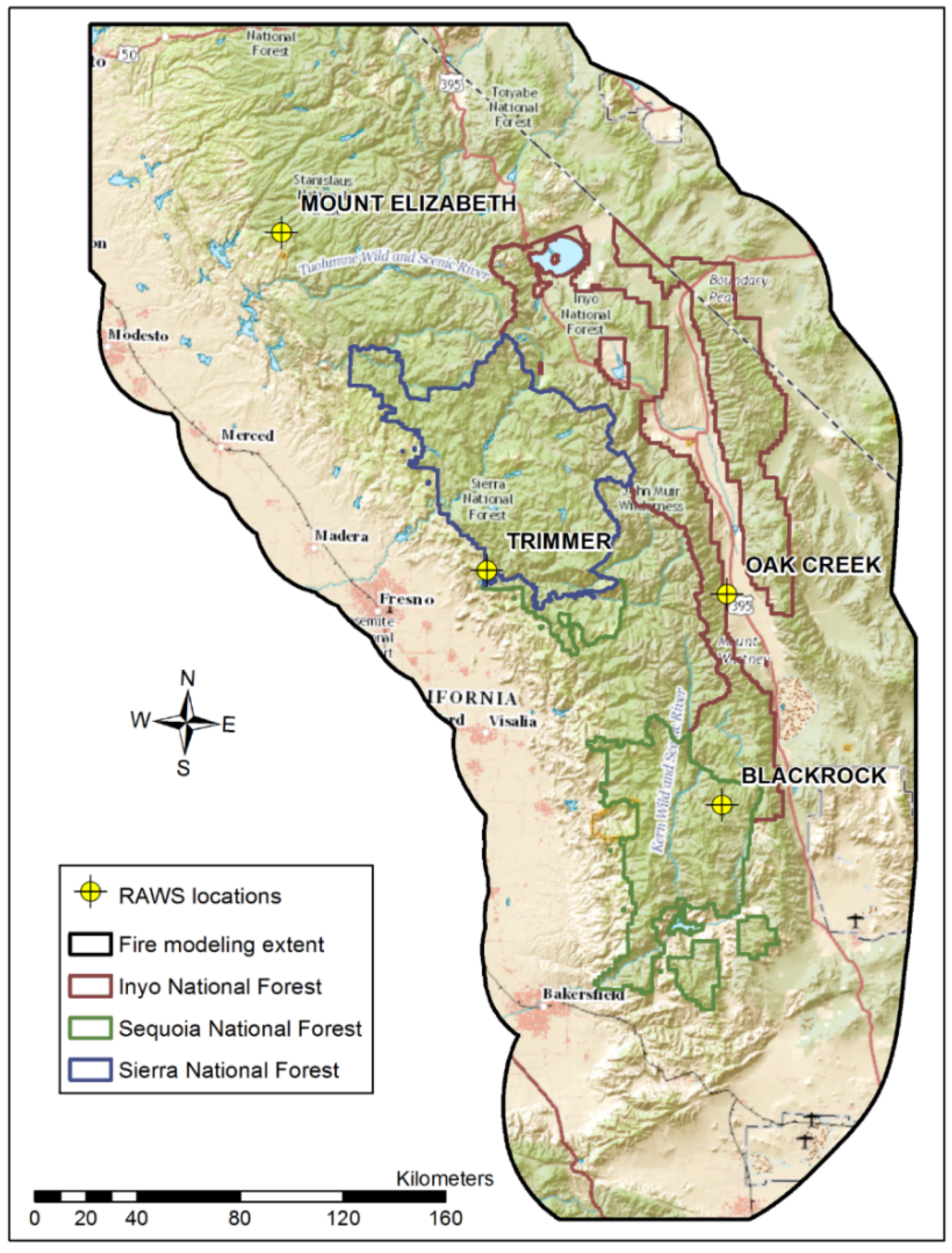
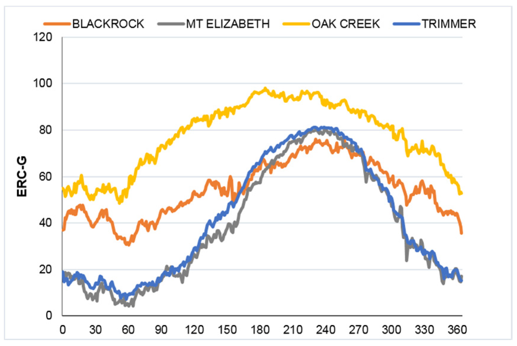
After reviewing data available from scores of RAWS stations across the landscape, we ultimately identified four RAWS stations to use for historical fire weather data across the landscape: Blackrock (044722), Oak Creek (044804), Mt. Elizabeth (043605), and Trimmer (044510). These stations are located in relatively representative locations (Figure 4) and have a relatively complete and long-duration record of historical weather. Each RAWS was used for one or more FOAs (Table 1). The historical data for each RAWS were used to generate results for use in the fire modeling system described in the next section.

3.4. Wildfire Simulation

For this analysis we used the FSim large-fire simulator [26] to quantify wildfire hazard across the landscape at a pixel size of 180 m (3 ha per pixel). FSim is a comprehensive fire occurrence, growth, behavior, and suppression simulation system that uses locally relevant fuel, weather, topography, and historical fire occurrence information to make a spatially resolved estimate of the contemporary likelihood and intensity of wildfire across the landscape [26]. Due to the highly varied nature of weather and fire occurrence across the large landscape, we ran FSim for each of the eight FOAs independently, and then compiled the 8 runs into a single coherent result using the method described in Thompson et al. [27]. For each FOA, we parameterized and calibrated FSim based on the location of historical fire ignitions within the FOA, which is consistent with how the historical record is compiled. We then used FSim to start fires only within each FOA, but allowed those fires to spread outside of the FOA. This, too, is consistent with how the historical record is compiled. Because fires are restricted to igniting within a FOA and growing into adjacent FOAs, the perimeter results from each FOA can be merged in a GIS without additional calculations. Some of the useful attribute fields attached to each fire perimeter include x and y coordinates of the ignition location, start-day Energy Release Component (ERC), start-day percentile ERC, and final fire size.

FSim requires information regarding historical weather. We used the four RAWS identified in the previous section for the necessary weather inputs. Weather data for these RAWS were used to produce monthly distributions of wind speed and direction, season-long trends of mean and standard deviation of ERC for National Fire Danger Rating System (NFDRS) fuel model G (hereinafter called ERC-G), and values for 1-, 10-, and 100-h timelag dead fuel moisture content associated with the 80th, 90th and 97th percentile conditions. These inputs are captured in FSim’s FRISK file.

FSim also requires information regarding the contemporary historical occurrence of fire in the analysis area, specifically large fires—those that escape initial attack and require extended suppression response. For each FOA we used the summaries of historical occurrence described above to parameterize and then calibrate FSim. Historical fire occurrence was not uniform across the fire modeling area—large fires were more likely to occur in some portions of the landscape than others. To account for that spatial non-uniformity, FSim uses a geospatial layer representing the relative ignition density across the landscape. FSim randomly locates wildfires according to this density grid during simulation. As described above, we made two ignition density grids (IDGs) using the ArcGIS-Spatial Analyst density tools with a 2-km cell size and 30-km search radius.

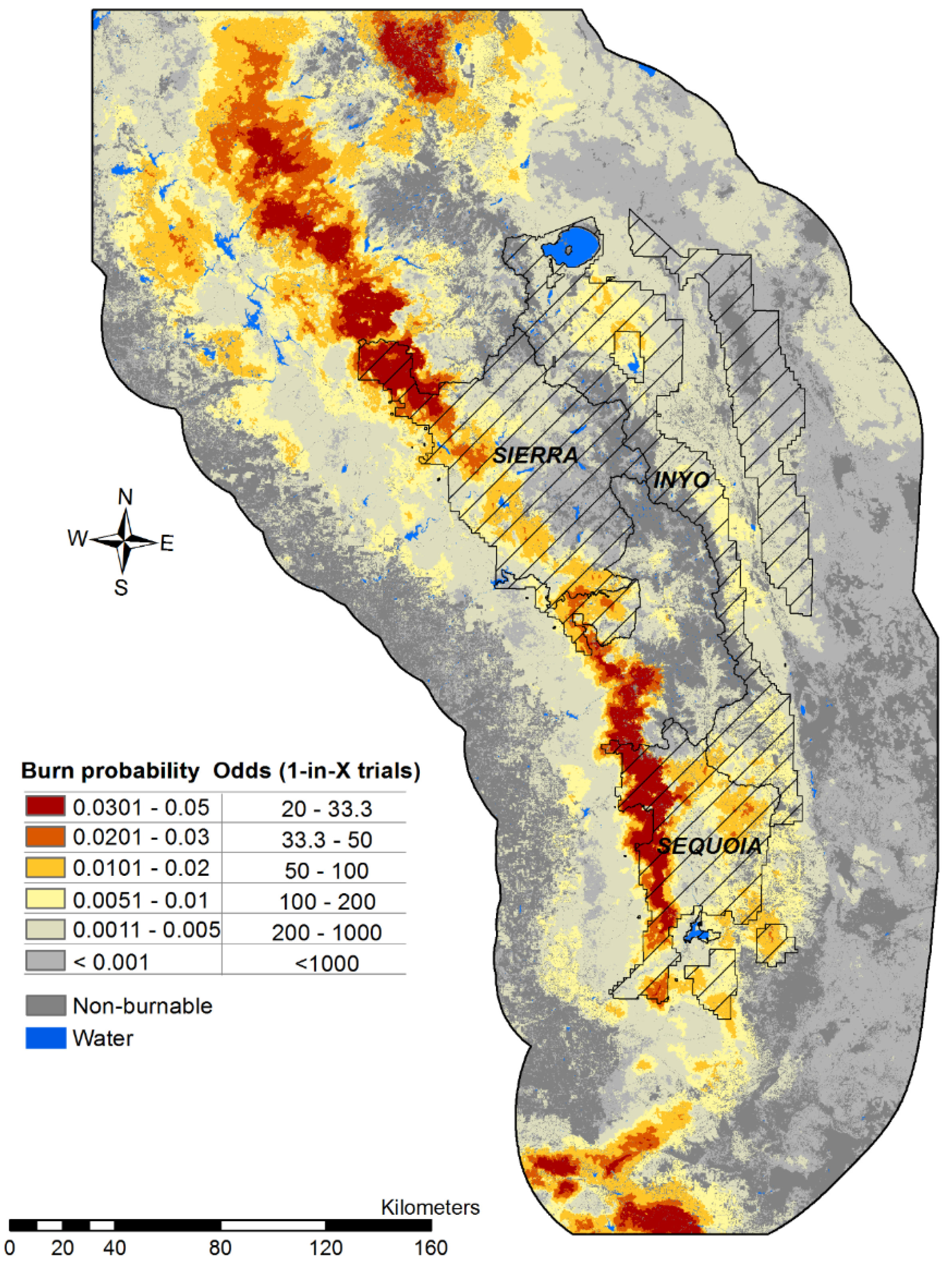
FSim simulations for each FOA were calibrated to historical measures of large fire occurrence including: mean historical large-fire size, mean annual burn probability, mean annual number of large fires per million hectares, and mean annual area burned per million hectares. From these measures, two calculations are particularly useful for comparing against and adjusting FSim results: (1) calculations of mean large fire size indicate whether simulated fires need to be larger or smaller on average; and (2) number of large fires per million hectares indicates whether FSim has simulated enough fires to match the annual frequency of large fires demonstrated by the historical record.

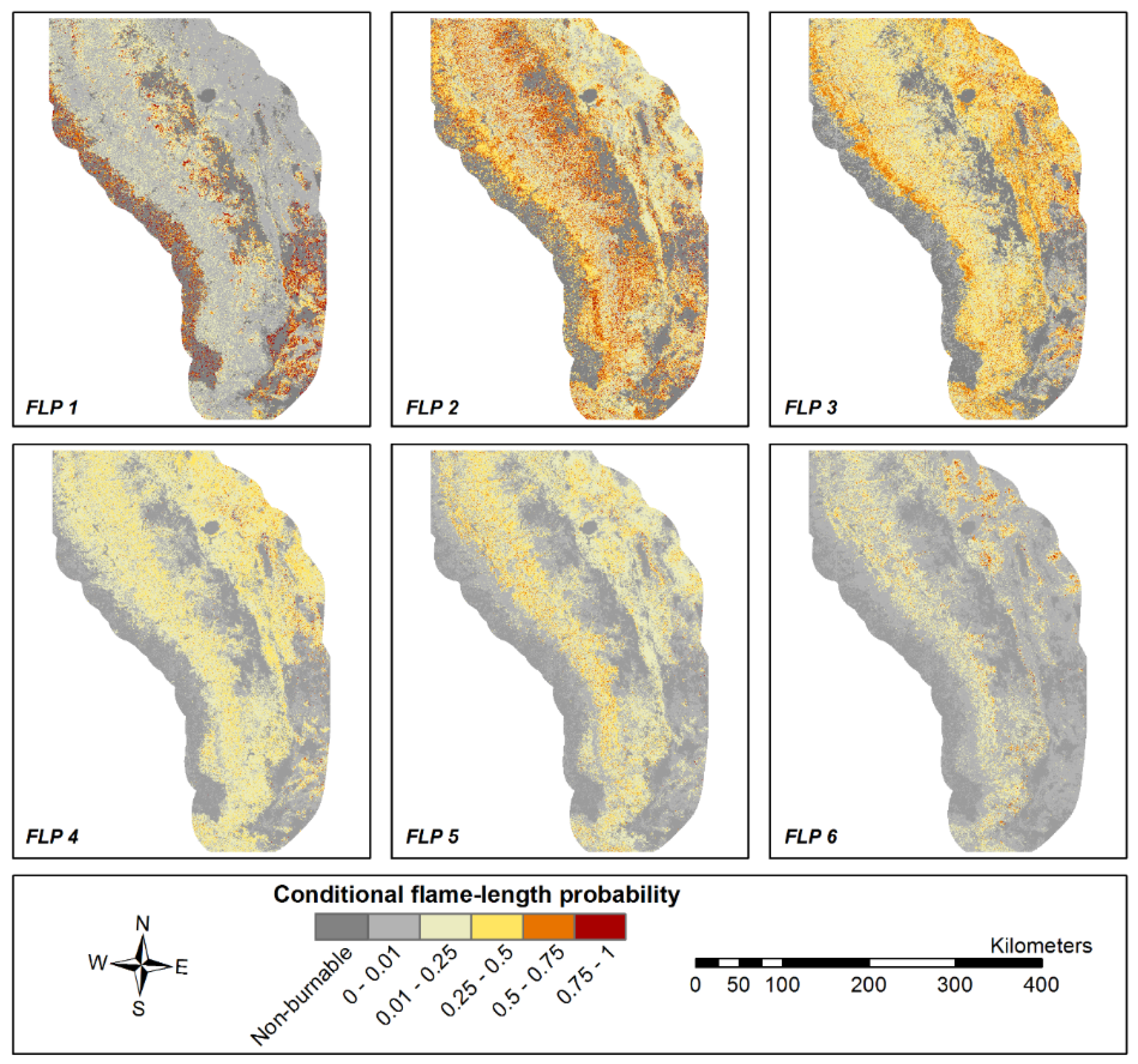
After calibrating FSim for each FOA independently, the final FSim runs included 10,000 years of simulated fire behavior results including annual burn probability, flame-length probabilities at each of the six flame-length categories, and fire perimeter polygons. We combined the results into a single landscape-wide result where the area-wide burn probability is simply the sum of all eight FOAs, and flame-length probabilities are weighted by their respective FOA burn probability and summed across all FOAs as described in Thompson et al. [27]. We then resampled the compiled 180 m results to a 90 m pixel size to match the resolution of the HVRA spatial layers. Using a 90 m fuel model grid, we identified any burnable pixels with zero burn probabilities resulting from the resample to a finer pixel size. To populate these pixels with an appropriate value, we used a moving-window smoothing to calculate the mean burn probability for all burnable pixels on the 90-m landscape, and then used these results to back-fill any remaining burnable pixels with a non-zero burn probability. This same approach was used for both annual burn probability and the six flame length probability grids.

A flame length probability grid represents the conditional probability that the flame length will be within a given flame length class. The flame length probability estimates are conditional, in the sense that they quantify probabilities given that the cell burns—simulation runs that don’t burn the cell are ignored in conditional flame length probability calculations. At a given location, the sum of the six flame length probability values necessarily equals 1.0. For our purposes here flame lengths are particularly important for estimating fire effects to HVRAs.

3.5. HVRA Characterization

The HVRAs assessed in the SSRA were selected and characterized by an ad hoc interdisciplinary team comprised of resource specialists, fire staff, and leadership team members from the three National Forests and the Region. The characterization of HVRAs is a multi-step process that includes generating maps of HVRA locations, estimating potential fire effects by defining HVRA-specific response functions (RFs), and assigning HVRA-specific relative importance (RI) weights [13]. RI weights range from 1 to 100, with 100 indicating highest importance (an RI value of 0 would imply that the HVRA should be excluded from the assessment). This approach is now widely used by the US Forest Service and has been implemented at national, regional, and forest-level scales ([14,15,16].

The SSRA included the following HVRA categories: visual resources (e.g., scenic byways), recreation and administrative infrastructure (e.g., ski resorts), major infrastructure (e.g., transmission lines and communication sites), inholdings (e.g., private industrial and state forests), where people live, critical terrestrial habitat (California spotted owl, northern goshawk, fisher, and sage grouse), timber resources, and watershed resources. Each HVRA was characterized by one or more data layers of sub-HVRA and, where necessary, further categorized by an appropriate covariate. Covariates include data such as erosion potential categories, age class of habitat (mature versus immature), and population density classes, the inclusion of which allows for refined estimation of potential fire effects and/or relative importance.

Local resource specialists produced a tabular RF for each HVRA category listed above. RFs are tabulations of the relative change in value of an HVRA if it were to burn in each of six flame-length classes (i.e., each HVRA is assigned a response value for each flame length class) A positive value in a response function indicates a benefit, or increase in value; a negative value indicates a loss, or decrease in value. Response function values ranged from −100 (greatest possible loss of resource value) to +100 (greatest increase in value). In order to integrate HVRAs with differing units of measure (for example, habitat vs. homes), relative importance (RI) values were assigned to each HVRA by members of the forest leadership teams for the three Southern Sierra National Forests. Relative importance values were developed by first ranking the HVRAs then assigning an RI value to each. The most important HVRA was assigned RI = 100. Each remaining HVRA was then assigned an RI value indicating its importance relative to that most-important HVRA. Relative Importance rankings for the three forests were combined into a single set of rankings by the fuel planning staff, and then adjusted as needed to ensure consistency within the analysis. These components are used along with fire behavior results from FSim in the conditional net value change (cNVC) and expected net value change (eNVC) calculations introduced in the next section.

Although each assessment is unique and reflects factors like data availability and management context, RFs and RIs were qualitatively similar to other assessments (e.g., [13,15]). For brevity we present only the maximum (best case) and minimum (worst case) RF values for each HVRA category to convey the range of possible losses and benefits (

Table 2. Maximum (best case) and minimum (worst case) Response Function values for all major HVRA categories.

HVRA	Best Case	Worst Case
Where people live	−5	−100
Inholdings	+50	−100
Major infrastructure	0	−40
Recreation infrastructure	0	−100
Visual resources	+70	−100
Terrestrial habitat	+90	−100
Timber	+45	−100
Watersheds	+20	−100

); additional information is available from the authors upon request. In nearly all cases the worst case is a complete loss of value, apart from major infrastructure which was determined to have higher resistance to loss. Whereas assets generally saw a best case of neutral or very low loss levels, many resources were expected to benefit from exposure to fire, particularly terrestrial habitat. In most cases these high benefit levels were from exposure to low intensity fire.

In addition to the HVRAs listed above, the SSRA also assessed the expected effects of wildfire on vegetation structure following the methods described in Scott et al. [28]. This is a custom approach separate from how fire effects are estimated for all other HVRAs. We mapped 15 biophysical setting (BpS) models selected from the LANDFIRE BpS dataset [29] along with their respective successional classes (S-Classes) present on the landscape. This approach uses the six flame-length classes produced by FSim to outline S-Class transition rules for fires burning at a given intensity. Each BpS/S-Class combination has a status within its respective landscape stratum, relative to historical reference conditions. Experiencing fire of a given flame length transitions a BpS/S-Class from one status to another, and the RF captures the net value change associated with a transition from one status to another. As an example, a transition from surplus to deficit would be strongly positive (+100), whereas a transition from deficit to surplus would be strongly negative (−100).

3.6. In Situ Risk Calculations

The next step is to characterize wildfire risk, quantified here using the concept of net value change, or net response, of each HVRA to fire [13,30]. Results are limited to those pixels or grid cells that have at least one HVRA and a non-zero probability of burning, i.e., there is no risk without probability of burning or potential consequences to an identified HVRA. 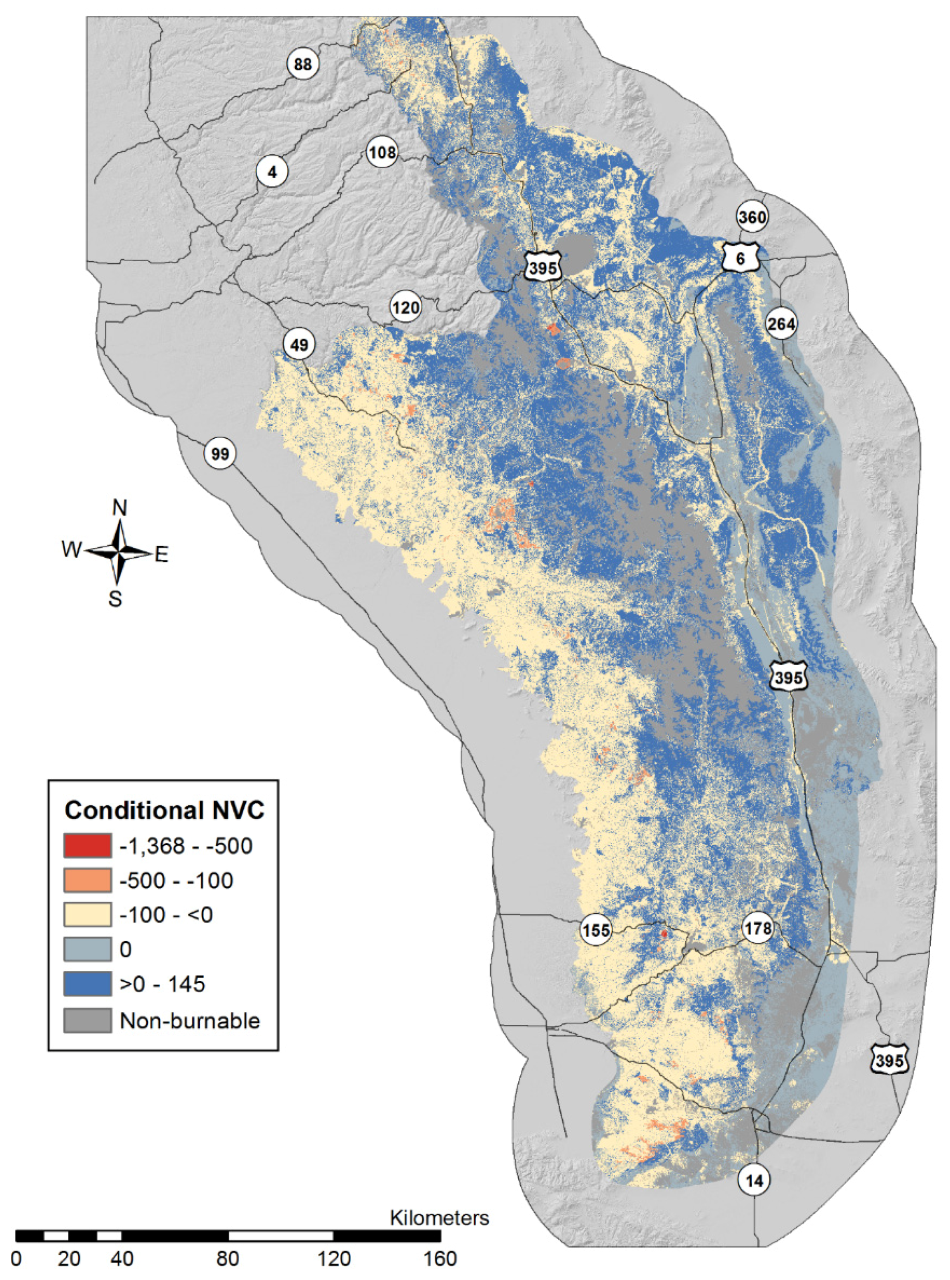A commonly used risk metric is expected net value change (eNVC), which reflects potential consequences weighted by the likelihood of fire occurring. Here our focus however is planning for response given a fire occurs, and so we are more interested in the conditional net value change (cNVC).

The in situ risk calculations produce spatial grids of cNVC and eNVC to all HVRAs. These metrics integrate potential losses and benefits across all HVRAs in the same terms, in effect allowing for an apples-to-apples comparison. To do so some additional calculations related to weighting are required. The RI values apply to the overall HVRA on the assessment landscape as a whole. The calculations need to take into account the relative extent of each HVRA to avoid overemphasizing HVRAs that cover many acres. This was accomplished by normalizing the calculations by the relative extent (RE) of each HVRA in the assessment area. Here, relative extent refers to the number of 90-m pixels mapped to each HVRA. In using this method, the relative importance of each HVRA is spread out over the HVRA’s extent. An HVRA with few pixels can have a high importance per pixel; and an HVRA with a great many pixels has a low importance per pixel. A weighting factor (WF) representing the relative importance per unit area was calculated for each HVRA.

The RF and WF values were combined with estimates of the conditional flame-length probability (FLP) in each of the six flame-length classes to estimate cNVC as the sum-product of flame-length probability (FLP) and response function value (RF) over all the six flame-length classes, with a weighting factor adjustments for the relative importance per unit area of each HVRA, as follows:

$$cNV{C}_j={{\displaystyle \sum }}_i^{n}FL{P}_i\times R{F}_{ij}\times W{F}_j$$

(1)

where i refers to flame length class (n = 6), j refers to each HVRA, WF is the weighting factor based on the ratio of the relative importance to the relative extent (number of pixels) of each HVRA. The cNVC calculation shown above places each pixel of each resource on a common scale (relative importance), allowing them to be summed across all resources to produce the total cNVC at a given pixel.

$$cNVC={{\displaystyle \sum }}_j^{m}cNV{C}_j$$

(2)

where cNVC is calculated for each pixel in the analysis area (m). Finally, eNVC for each pixel is calculated as the product of cNVC and annual BP:

$$eNVC=cNVC\times BP$$

(3)

To reiterate, our focus here is on cNVC calculations, so we provide the equation for eNVC calculations for the sake of completeness.

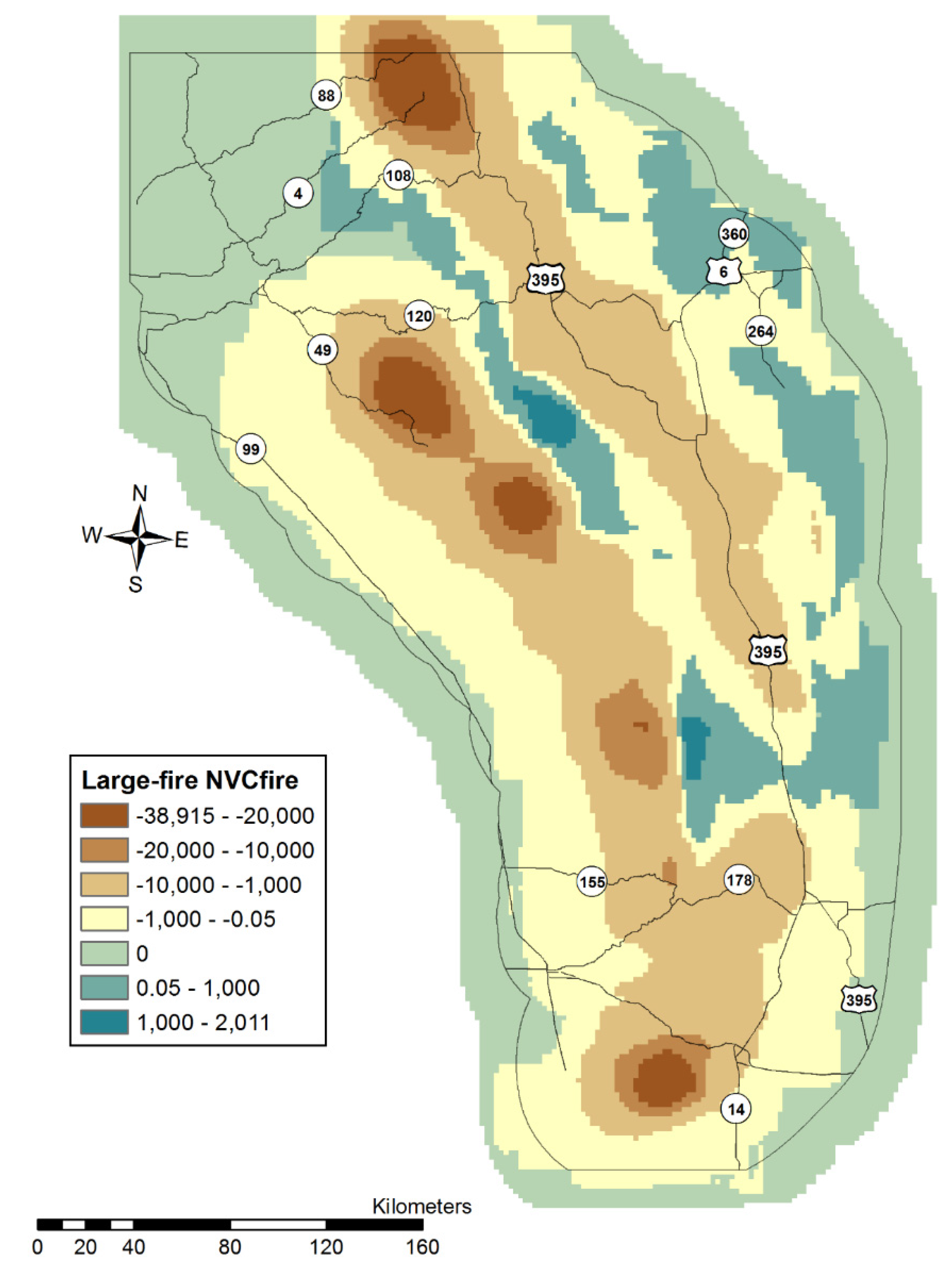
3.7. Source Risk Calculations

Risk-source maps combine both pixel-based risk assessment results and fire perimeter polygons to identify each fire’s potential for positive or negative outcomes, and tie that information back to the fire’s ignition to identify spatial patterns on the landscape. Thus identifying the source of risk to HVRAs requires fire perimeter polygons simulated by FSim, as well as the cNVC grid produced from the effects analysis above. The total NVC for a given fire (NVC_fire) is calculated as the sum of cNVC of each pixel (k) that fell within a simulated fire perimeter (z = total number of pixels in perimeter), as shown in the equation below.

$$NV{C}_{fire}={{\displaystyle \sum }}_k^{z}cNV{C}_k$$

(4)

We calculated NVC_fire for every fire perimeter on the landscape using the zonal statistics function of the RMRS Raster Utility Tool [31] which allows for efficient summation of all pixels contained by a given perimeter (or summary zone), regardless of the other fire perimeters it overlaps. NVC_fire is then assigned back to that fire’s ignition location, for every ignition on the landscape to create a point feature layer with NVC_fire at each point. The points are then plotted using a smoothing approach to identify the broader trends emerging from 10,000 years of simulated fire data. This exercise was completed for both large fire and lightning-caused simulated fires.

3.8. Defining PODs and Response Categories

PODs are a spatial representation of an area useful for summarizing risk in a meaningful operational fire management context. PODs can also identify priority fuel treatment projects, within a given POD or along the seams between PODs with different risk levels and response categories. PODs can be spatially delineated using coarse approximations like 6th level sub-watersheds, or with more refined fire operation features such as ridgetops, waterbodies, roads, barren areas, elevation changes, or major fuel changes. Areas of significant change in wildfire hazard and risk could also inform POD boundary decisions. Determining POD boundaries is an iterative process driven by questions such as how fire would be managed within the area, how and why response might be different within a given area, and whether the POD size is consistent with a realistic scale of fire management operations. Here we use PODs as the spatial unit of analysis for strategic response zones.

POD boundaries are not intended to be set-in-stone, but rather an approximation of an area that would be used to manage fire. For instance an area may have multiple roads that could serve as control points, any of which could be used operationally rather than the specific road selected to form the POD boundary. Some mapped boundaries may not be an ideal boundary in the real world, for instance a narrow ridge might not under some conditions be an effective barrier to spread or a safe location to place firefighters. It is critical therefore that PODs are developed with local knowledge including fire specialists, fire and fuel planners, GIS specialists, and resource specialists, along with leadership. POD delineation may also entail working with neighboring landowners, particularly with respect to how fires might be managed across boundaries.

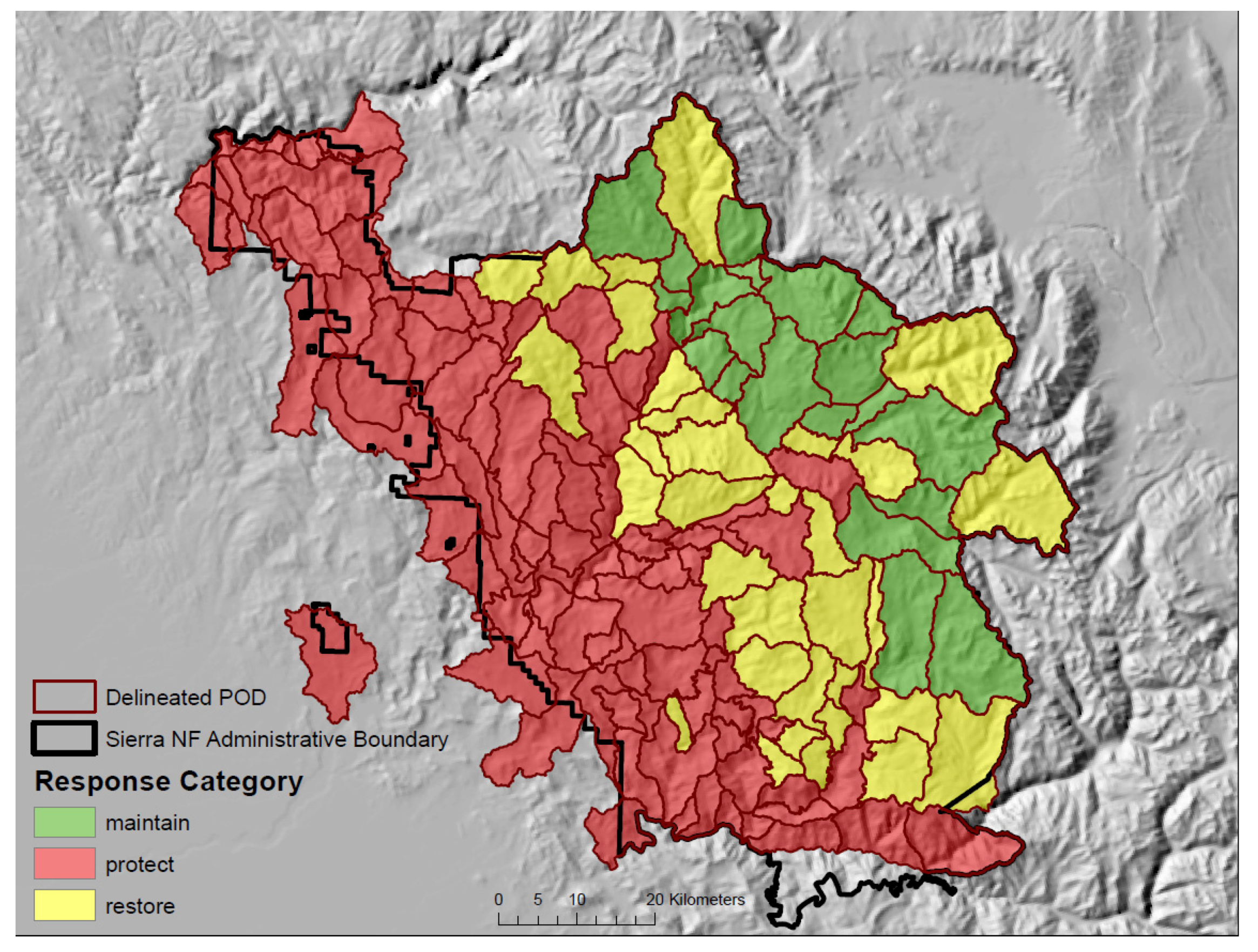
To demonstrate, we drill down and use a set of 147 PODs selected according to the criteria of having at least 10% of the area within the administrative boundaries of the Sierra National Forest, exclusive of the Great Sequoia National Monument. We developed these POD boundaries using a process patterned after one implemented by the local fuels planner on the Inyo National Forest (part of the SSRA). Reflective of landscape heterogeneity, PODS varied in size and shape, with a mean size of 4281 ha, and a median size of 3069 ha, which roughly corresponds to 2–3 PODs per 6th level sub-watershed. Note that the PODs we use here for purposes of demonstration may be updated by the Forests in the future, i.e., POD boundaries are not necessarily a finished product. In fact, as a design feature POD boundaries should be flexible, for instance in response to significant fuel changes after a large disturbance event.

Lastly, we define our schema to assign each POD to one of the three aforementioned response categories. This categorization is based on the combination of in situ risk and source rick cNVC calculations. We use cNVC rather than eNVC because incident response decisions are ultimately conditional on the occurrence of a fire. By contrast, eNVC values that incorporate the probability of burning might be quite useful for prioritizing PODs for mechanical fuel treatment or prescribed burning. Our schema uses a simple breakdown that sums cNVC within each POD and determines whether the POD-level risk total represents a net loss (−) or a net benefit (+). Other categorization schemas could be defined, for instance using alternative numerical thresholds for assignment based on cNVC values.

Table 3. Schema for assigning Potential wildland fire Operational Delineation (POD)-level response categories based on in situ and source risk calculations.

Response Category	In Situ cNVC	Source cNVC
Protect	−	−
Restore	−	+
	+	−
Maintain	+	+

summarizes our assignment of categories based on net loss/benefit calculations. If in situ risk and source risk are a net loss, the POD is assigned “protect.” If in situ risk and source risk are a net benefit, the POD is assigned “maintain”. The “restore” category is assigned where in situ risk and source risk are mixed.

4. Results

4.1. Historical Wildfire Occurrence

The historical annual number of large fires, mean large-fire size, and annual area burned varied widely by FOA (

Table 4. Summary of historical mean annual number of fires per million hectares, mean size of large fires, and mean large-fire annual area burned per million hectares by fire occurrence area (FOA).

FOA	Annual Number of Large Fires (per Million Hectares)	Mean Large-Fire Size (Hectares)	Annual Area Burned (per Million Hectares)
1	14.55	1010	14,696
2	7.64	1383	10,559
3	3.78	2437	9212
4	2.27	869	1975
5	5.71	770	4394
6	3.51	923	3240
7	11.07	927	10,264
8	2.42	1743	4221

). A general trend of high numbers of large fires and annual area burned for FOAs in the lower elevations is apparent (e.g., FOAs 1, 2, and 7). However, FOAs covering higher elevations and those on the eastern side of the Sierras tend to have fewer fires and typically burn less area annually. FOA 3 is an exception to this trend, with an average fire size of 2437 hectares and 9212 hectares burned annually (per million hectares). Overall, FOA 1 ranks highest in terms of number of fires and annual area burned. FOA 7 ranked second for number of large fires, but on average those fires burned less area on a relative basis (10,264 hectares). FOA 4 had the lowest number of large fires (2.27) and burned the least number of hectares annually (1975). The wide range of historical occurrence shown in Table 4 underscores the need for distinct FOAs for fire modeling in diverse geographic areas with highly variable fire histories.

4.2. Historical Weather

Our historical weather analysis yields two files used by FSim for simulating historical weather and determining the weather characteristics that produced large fires historically, the FDist and the FRISK files. The FDist file provides FSim with logistic regression coefficients that predict the likelihood of a large fire occurrence based on the historical relationship between large fires and ERC and tabulates the distribution of large fires by large-fire day. A large-fire day is a day when at least one large fire occurred historically. The information contained in the FDist file is summarized by FOA in

Table 5. Logistic regression coefficients and mean number of large fires per large-fire day, summarized by fire occurrence area (FOA).

FOA	Logistic Regression Coefficients		Mean Number of Large Fires per Large-Fire Day
	a	b
1	−6.406	0.047	1.32
2	−6.526	0.040	1.15
3	−13.091	0.082	1.04
4	−7.342	0.034	1.01
5	−7.478	0.032	1.08
6	−6.769	0.025	1.06
7	−4.545	0.026	1.09
8	−10.359	0.060	1.13

. On average, the majority of large fires occur on a single day, however, in some FOAs there is a greater chance of having multiple large-fire starts on a single day. FOAs 1, 2, and 8 have the highest likelihood of more than one fire occurring, with average number of large fires per large-fire day of 1.32, 1.15, and 1.13, respectively.

The logistic regression coefficients together describe large-fire day likelihood P(LFD) at a given ERC-G as follows:

$$P\left(LFD\right)=\frac{1}{1+ e^{-a + \left(-b \times ERC\left(G\right)\right)}}$$

where a and b are listed in Table 5.

The FRISK file captures and summarizes weather information from the RAWS station. Specifically, ERC values and descriptive statistics for each day of the year are compiled for all years of available record. Using the mean ERC-G value corresponding to each Julian day of the year, we compare ERC-G between the four RAWS stations used in the FSim fire modeling (Figure 5). The two stations west of the Sierra crest—Trimmer and Mount Elizabeth—show very similar mean ERC-G values throughout most of the year. The stations to the east have less seasonal variability. The weather module in FSim uses these daily ERC-G values together with percentile ERC-G to simulate thousands of historical weather years. Additionally, wind data described as the joint probability of wind speed and direction are summarized by month in the FRISK file and sampled at random by FSim and combined with ERC-G data to create thousands of simulated weather scenarios.

4.3. Wildfire Simulation

FSim produced wildfire hazard results for each FOA including burn probability and conditional flame length probability grids. We combined the eight FOAs using the calculations described above to produce integrated maps of wildfire hazard for the entire fire modeling area. Burn probability in the risk assessment area ranges from less than 0.001 (1 in 1000 odds) to 0.05 (1 in 20 odds) at the highest (Figure 6). The highest burn probabilities are typically found on the western side of the Sierra crest, predominately in the zone where vegetation transitions from grass and shrub to timber. These results mimic historical patterns of large fires observed in the area. Mean annual burn probability is 0.007 (1 in 142 odds).

Conditional flame-length probabilities are mapped for the assessment area in Figure 7. These maps indicate the likelihood of flame-lengths at each intensity level and their associated spatial distribution, as influenced by spread direction and variability in wind speed and direction as well as fuel moisture. Grid values range from 0 to 1 in each panel and are mapped with grey for lower probabilities to red for values closer to 1. Note it is these values, rather than burn probabilities, that are used in cNVC calculations, as described in the methods section. Flame lengths are lowest in the valley bottoms and lower elevations where vegetation is typically shorter (i.e., grass and grass/shrub) and along the Sierra crest in the alpine zone where vegetation is shorter and fires tend to burn under very moderate conditions. Flame lengths are greatest in the shrub and timber fuels west of the Sierra crest and in the northeastern shrub fuel models.

In addition to wildfire probability and intensity grids, FSim produces polygon shapefiles of all fire perimeters generated in the simulation. Perimeters are used in the risk source calculations.

Table 6. Large-fire simulation results summarized by fire occurrence areas (FOA).

FOA	Annual Number of Large Fires (per Million Hectares)	Mean Large-Fire Size (Hectares)	Annual Large-Fire Area Burned (per Million Hectares)
1	9.61	2228	21,402
2	7.99	2963	23,685
3	3.64	4466	16,237
4	1.92	2066	3960
5	5.46	1300	7092
6	3.25	1481	4814
7	9.15	1072	9808
8	2.42	2242	5420

summarizes large fire (to reiterate, greater or equal to 100 ha) results from the final fire perimeters originating within a given FOA. Consistent with the historical occurrence, FOA1 had the greatest number of large fires (9.61) but second-greatest area burned by large fires at 21,402 hectares annually. FOA7 had a similar number of large fires annually, but those fires were much smaller and resulted in significantly less area burned (9808 hectares). Just as for historical occurrence, FOA4 had the least number of fires (1.92) and the lowest annual area burned by large fires (3960 ha). Despite the low number of annual large fires and moderate annual area burned, FOA3 had the largest mean large-fire size at 4466 ha, which is also consistent with the historical occurrence.

4.4. In Situ Risk Calculations

Figure 8 shows cNVC results across the assessment area, with beneficial effects shown in blue and negative effects in warmer colors like orange and red. Much of the timber fuel in the middle of the assessment area and the shrub fuel along the northeastern portion experience positive conditional fire outcomes—should a fire occur—while the majority of the western portion of the assessment area resulted in negative outcomes. Positive fire effects are largely attributable to beneficial responses for certain BpS models where fire had the desired effect of creating a distribution of SClass categories more representative of desired conditions. Conversely, negative values seen along the western portion of the assessment area represent negative outcomes to watersheds, human habitation and infrastructure, slightly reduced by some positive outcomes due to vegetation. At first glance, it appears there are more beneficial effects on the landscape than there are negative. However, the overall mean cNVC value for the landscape is slightly negative at −0.57. Pixel values of negative outcomes range from less than zero to −1368 while positive outcomes have a max value of 145. Although there are relatively few areas of orange and red pixels, their values could be up to nine times the value of a beneficial outcome.

4.5. Risk Source Calculations

Figure 9 is a plot of smoothed, NVC_fire for large-fire ignitions and large-fire cNVC. To reiterate, NVC_fire values are conditional on large fire occurrence (unweighted by ignition probability), and represent the cumulative impacts of each simulated large fire. This figure differs from Figure 8 in that here we can generally identify where on the landscape fire ignitions tend to result in negative versus positive outcomes. Specifically, aggregated over 10,000 simulations, the average result of fires that start west of the Sierra crest is slightly negative to highly negative. The same is true of fires that start in the northern-most portion of the assessment area, extending down into west side of the range. Conversely, fires that start in the middle of the assessment area, where cNVC tends to be positive, result in positive outcomes, on average. This is also the case for fires igniting along the northeastern and eastern area-boundaries.

4.6. PODs and Response Categories

In terms of response category assignments, 93 PODs were “protect”, 34 were “restore”, and 20 were “maintain”. The magnitude of net losses and benefits is different across POD assignments, and across types of risk calculations (

Table 7. Summary statistics for POD-level in situ and source risk calculations, quantified in terms of conditional net value change (cNVC), and broken down according to response category; values presented in parentheses are negative.

Descriptive Statistics	In Situ cNVC	Source cNVC
Protect (n = 93)
Mean	(54,002)	(15,240)
Standard Deviation	78,540	8036
Min	(563,117)	(32,080)
Max	(189)	(91)
Restore (n = 34)
Mean	13,779	(6679)
Standard Deviation	15,937	7050
Min	(9774)	(24,205)
Max	56,816	608
Maintain (n = 20)
Mean	15,294	699
Standard Deviation	12,142	448
Min	1214	65
Max	44,551	1509

). The “protect” category has the highest conditional net losses for both in situ and source risk calculations, as well as the highest variability. Across categories, the absolute magnitude of mean net losses exceeds that of mean net benefits, which reflects the susceptibility and high importance of the wildland-urban interface, among other factors. Absolute magnitudes for in situ risk calculations are greater than that of source risk calculations in all cases, which simply reflects the greater number of fires included in the calculations; in situ risk includes not only fires that ignited within a given POD, but also fires that ignited elsewhere and spread into the given POD (i.e., in situ risk is a function of source risk from other PODs on the landscape).

At least three notable patterns emerge from the POD assignments. First, unsurprisingly, the wildland-urban interface was a major driver—of 85 PODs that contained any mapped wildland-urban interface, 73 were assigned “protect” and 12 were assigned “restore”. None of the PODs in the “maintain” category had any mapped wildland-urban interface. Of the PODs containing wildland-urban interface, the average estimated population in the “restore” category was more than two orders of magnitude lower than that in the “protect” category. This suggests that assigning the “restore” category with some measure of tolerance for or even promotion of fire is only an option in PODs with very low population densities.

Second, the “restore” PODs have a mean net benefit for in situ risk, but a mean net loss for source risk calculations. Across the 34 PODs in this category, only 3 PODs had a net in situ loss, whereas 31 PODs were a net source loss. This result is principally a function of being adjacent to PODs that fell into the “protect” category with a greater concentration of HVRAs with negative responses to fire. That in situ results are overwhelmingly positive suggests that within-POD prescribed burning or managing natural fire under conditions suitable to high probability of control might lead to significant net benefits.

Third, the spatial mosaic of POD response assignments tends to follow an easterly progression from “protect” to “restore” to “maintain” (Figure 10). Proximity to the wildland-urban interface along the western flanks of the Forest boundary clearly plays a strong role here. So too does the potential for “restore” PODs to act as a source of net loss to adjacent PODs within the “protect” category, as mentioned above. “Maintain” assignments by contrast tend to be the furthest from development, where the principal HVRAs impacted by fire are natural resources, and where fire can improve vegetation condition. Note that there are three “maintain” PODs that abut “protect” PODs, which suggests that the potential for local ignitions to spread beyond POD boundaries is minimal within these specific “maintain” PODs.

5. Discussion

In this paper we demonstrated how state-of-the-art spatial risk assessment can support spatial fire planning, and outlined a possible pathway for developing strategic response zones. We described how two spatial metrics of conditional wildfire risk can be helpful in better understanding and balancing the potential consequences of alternative responses to fire. In situ risk helps refine estimates of the consequences if the fire reached a certain location, and is reflective of local characteristics related to HVRAs, fuels, and terrain. This information can support, for instance, decisions related to locating control points, attempting to redirect fire spread, or assigning resources to point protection. Source risk provides a broader perspective of the propensity for fires that ignite in a given location to spread to areas with HVRAs. This can support decisions related to initial response strategies with information that is complementary to local risk concerns, particularly where local HVRA effects might be positive but fire could spread to areas prone to loss (i.e., “restore” zones).

We embedded the risk assessment in a broader strategic framework for response planning based on the conceptual Wildland Fire Management Continuum. This framework is premised on pre-fire assessment to support risk-informed decisions, while recognizing the need for flexibility and responsiveness to changing conditions. This framework is further premised on pre-fire assessment and planning in terms of features and considerations relevant to operational fire management. Hence the design of a spatial mosaic of PODs, within which we summarized in situ and risk source calculations. POD-level summaries of risk metrics can reduce uncertainty surrounding potential losses and benefits given large fire occurrence, and lend themselves naturally to design of fire and fuel management strategies. The spatial representation of fire hazard and risk, along with fire management objectives and options, should ideally provide a valuable tool for identifying strategic responses to wildfire that align with land and resource objectives.

While our intent here is to establish a basic foundation for response planning, a number of extensions and improvements are foreseeable or in development. The scope of fire modeling and risk assessment could be expanded, for instance simulating only lightning-caused ignitions and estimating their potential size and HVRA impacts if unsuppressed. This approach could establish benchmarks for risk source loss levels against which alternative response policies could be compared. Strategic response planning could spatially assign response categories at larger scales, in effect aggregating PODs based on coarser summaries of in situ and source risk. This would not, of course, mandate any particular response to ignition within a given zone, but could greatly simplify strategic assessment and planning at eco-regional or larger scales. Planning efforts could integrate eNVC in addition to cNVC values, particularly for fuel management questions where the likelihood of fire is a primary consideration. POD-level response planning could similarly use eNVC values, for instance to prioritize PODs for monitoring and maintenance of control features. POD features could be integrated directly into spatial fuel treatment design, for instance to reduce fire behavior and resistance to control along POD boundaries [32,33]. While here we took preexisting POD boundaries as fixed, future research could examine patterns and characteristics of POD features and evaluate alternative spatial POD designs. Lastly, in addition to risk metrics POD attributes could be characterized with indices of suppression difficulty or resistance to control (e.g., [34]).

The assessment and planning framework introduced here has several limitations and qualifications to note. First, large fires are low-probability, high-consequence events, with associated difficulties in prediction and the potential for bad outcomes despite good decisions. That exact ignition locations or fire weather conditions can’t be predicted does not mean, however, that general patterns can’t be discerned or that alternative scenarios can’t be considered in assessment and planning efforts. Second, the temporal scope of the risk assessment is short-term, and does not capture dynamics of succession and disturbance through time. Periodic assessment can at least partially offset this limitation, particularly in response to large disturbance events that might significantly alter spatial patterns of hazard and risk. Further, as mentioned earlier, POD boundaries and categories are flexible and could also be updated dynamically through time. Third, the fire modeling and risk assessment processes and products are subject to a variety of uncertainties and knowledge gaps, which are extensively discussed and characterized in reviews by Finney et al. [35], Hyde et al. [36], and Thompson and Calkin [37]. The assessment and planning process described here is premised on pairing appropriate modeling and decision support approaches with the type of uncertainties faced [16], and more broadly on iterative calibration, refinement, and reliance on local expert knowledge and experience.

To summarize, consider that fire management objectives are essentially a vector, or a means, by which underlying land and resource objectives can be achieved. Fire management actions and alternatives therefore must be evaluated in light of their impacts on desired conditions. The framework and process we introduce is one vehicle by which fire planning and ultimately fire response could be enhanced and directly tiered off of HVRAs and related concerns outlined in land and resource plans. Leveraging spatial risk assessment methods with fire planning helps more strongly infuse risk management principles into fire management decision making, and increases the likelihood of attaining the goals outlined in the Cohesive Strategy [8].