Article

Simulating Water-Use Efficiency of Piceacrassi folia Forest under Representative Concentration Pathway Scenarios in the Qilian Mountains of Northwest China

1
State Key Laboratory of Soil Erosion and Dryland Farming on the Loess Plateau, Northwest A & F University, Yangling 712100, China
2
Institute of Soil and Water Conservation, Chinese Academy of Sciences and Ministry of Water Resources, Yangling 712100, China
*
Author to whom correspondence should be addressed.
Forests 2016, 7(7), 140; https://doi.org/10.3390/f7070140
Submission received: 25 April 2016 / Revised: 21 June 2016 / Accepted: 7 July 2016 / Published: 12 July 2016
(This article belongs to the Special Issue Climate Change Impacts on the Dynamics of Forest Ecosystems)

Abstract

:
The current study used the Biome-Bio Geochemical Cycle (Biome-BGC) model to simulate water-use efficiency (WUE) of Piceacrassi folia (P. crassifolia) forest under four representative concentration pathway (RCP) scenarios, and investigated the responses of forest WUE to different combinations of climatic changes and CO2 concentrations in the Qilian Mountains of Northwest China. The model was validated by comparing simulated forest net primary productivity and transpiration under current climatic condition with independent field-measured data. Subsequently, the model was used to predict P. crassi folia forest WUE response to different climatic and CO2 change scenarios. Results showed that (1) increases in temperature, precipitation and atmospheric CO2 concentrations led to associated increases in WUE (ranging from 54% to 66% above the reference climate); (2) effect of CO2 concentration (increased WUE from 36% to 42.3%) was more significant than that of climate change (increased WUE from 2.4% to 15%); and (3) forest WUE response to future global change was more intense at high elevations than at low ones, with CO2 concentration being the main factor that controlled forest WUE variation. These results provide valuable insight to help understand how these forest types might respond to future changes in climate and atmospheric CO2 concentration.

Graphical Abstract

1. Introduction

The fifth assessment report (AR5) of the Intergovernmental Panel on Climate Change (IPCC) showed that the earth’s overall carbon dioxide (CO2) concentration has increased from 280 parts per million by volume (ppm) at the beginning of the Industrial Revolution in the 1850s to the present level of 400 ppm [1,2]. The report also projects that global surface mean temperature will increase by 1 °C–3.7 °C in the late 21stcentury relative to the 1986–2005 period under the various representative concentration pathway (RCP) scenarios [3]. These factors will likely result in significant changes in vegetation function over large fractions of the global land surface [4,5]. Forests cover nearly one-third of the earth’s land area and contain up to 80% of the total above-ground terrestrial carbon and 40% of below-ground carbon [6]. Therefore, understanding how forest ecosystems will respond to global changes in the future is imperative.
Although many studies have accounted for the effects of climate change on forest ecosystems, they have generally focused on responses of forest net primary production [5,7,8,9]. Water-use efficiency (WUE), net primary productivity (NPP) to transpiration ratio [10,11], has been identified as an effective integral trait for assessing ecosystem response to climate change [12]. While there have been several studies examining the potential effects of changes in atmospheric CO2 concentrations [13,14] and precipitation patterns [15,16] on water-use efficiency in forest ecosystems, the response of different forest types to alternative climate change scenarios remains unclear.
Piceacrassi folia forest, the most dominant and widespread subalpine forest in the Qilian Mountains of Northwest China, is typically distributed from 2500 m to 3300 m and forms pure stands in this region [17].This type of forest is tolerant to cold and dry climates [18] and provides key ecological services, including carbon sequestration, water quality, and water flow regulation [19]. Carbon storage in P. crassifolia forests, as well as transpiration rates and WUE, have been examined in several studies [20,21,22,23,24,25]. However, little is known with respect to the potential impacts of climate change and associated increases in atmospheric CO2 concentrations on P. crassifolia productivity and WUE.
In this study, we used the Biome-BGC model developed by Thornton et al. [26] to assess the effects of future climate and atmospheric CO2 concentration changes on productivity and WUE of P. crassifolia forest. The model was validated by comparing independent field-measured data with simulated NPP and transpiration values. Subsequently, the validated model was applied to explore the impacts of alternative RCP emission and climate change scenarios, as described in the IPCC AR5 report, on long-term patterns of productivity and WUE in P. crassifolia.

2. Materials and Methods
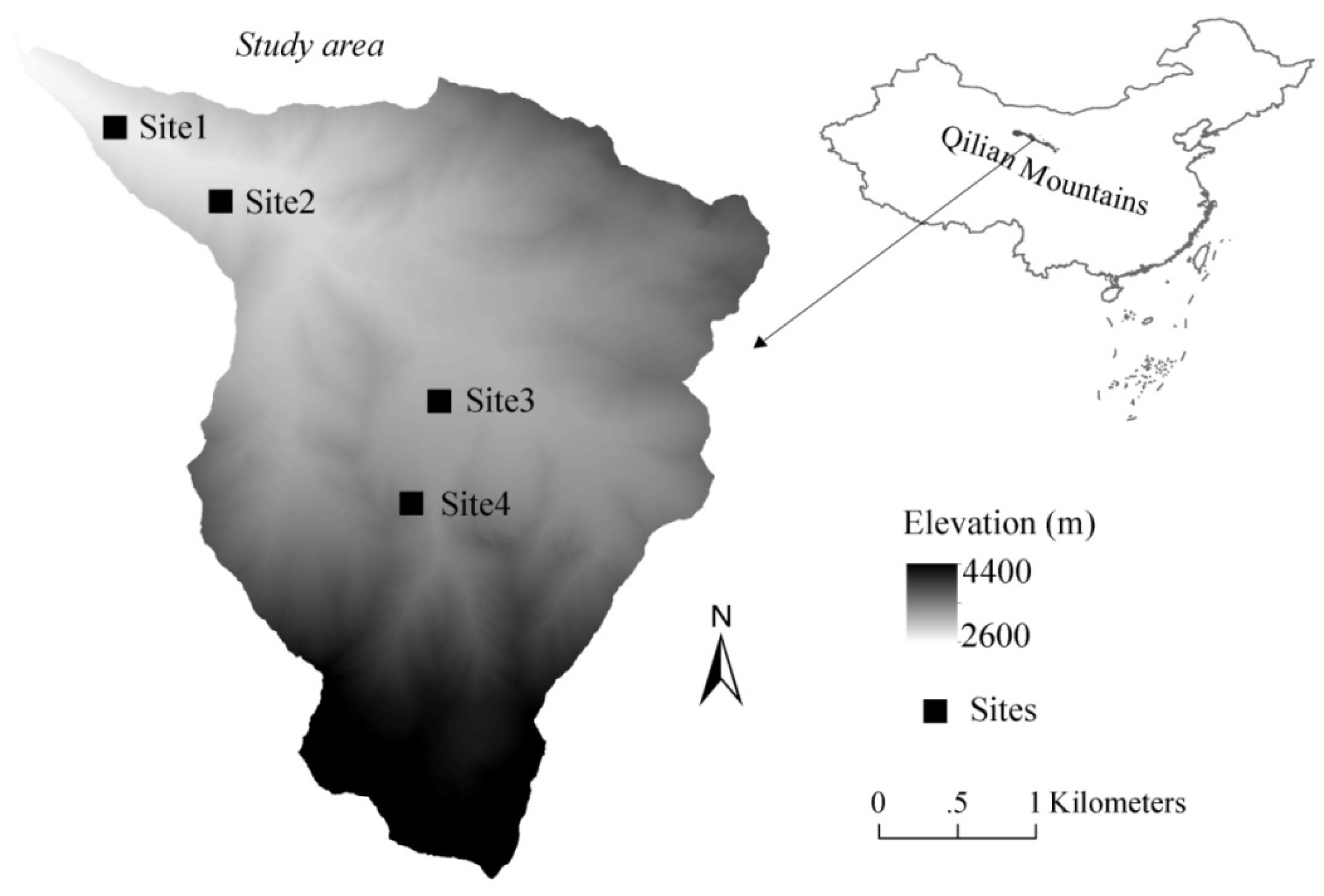
2.1. Study Sites

The study area lay in Tianlaochi catchment located in the middle part of the Qilian Mountains (Figure 1). Its elevation ranges from 2600 m to 4400 m, and its climate is characterized by cold and dry winters and cool and wet summers, which is the typical climate of Qilian Mountains. The vegetation types differ from lower to higher elevations and from north to south aspects. Specifically, the lower elevation belt from 2600 m to 3250 m is occupied by P. crassifolia forest in north aspects and by grassland in south aspects. The middle portion ranging from 3250 m to 3750 m is dominated by alpine shrubs, and the topmost portion above 3800 m is barren land. Four sites in P. crassifolia mature forest with different elevations were selected for this study (Figure 1). The sites are relatively undisturbed by either natural or anthropogenic factors and tend to be quite homogeneous. General characteristics of the sites are presented in Table 1.

2.2. Data Collection

In each site, one plot was established and the size of plot was equal to that of corresponding site. Field measurements were conducted in the study sites in September 2013 and April 2014. Diameter at breast height, 1.3 m, (DBH), and top height (H) were measured for all trees >5 cm DBH within the plot boundary. At least eight P. crassifolia trees in different diameter classes without visible signs of damage were randomly selected as sample trees to obtain representative increment cores for use in calculations of past productivity. Two increment cores for each selected tree were taken at 1.3 m above ground with an increment borer and stored in paper straws. Cores were glued on wooden blocks, dried for 24 h, polished with fine sandpaper, and then examined under a stereomicroscope. All growth rings were marked, and each annual ring width was measured using a video micrometer (Olympus VM-31, Tokyo, Japan) connected to the stereomicroscope. Ring-width data were used to determine past increments in tree diameter and subsequently to estimate biomass increment on individual trees.
Measurement of sap flow was conducted in Site3 using sap flow sensors with a modified heat-pulse velocity technique (SF-L, Ecomatik, Munich, Germany). Five Qinghai spruce individuals were selected with different DBH for the measurement in2013 and 2014. The sap flow data were used to estimate daily transpiration for the P. crassifolia forest, and then to validate the applicability of Biome-BGC in terms of transpiration simulation for P. crassifolia forest under current climate conditions.

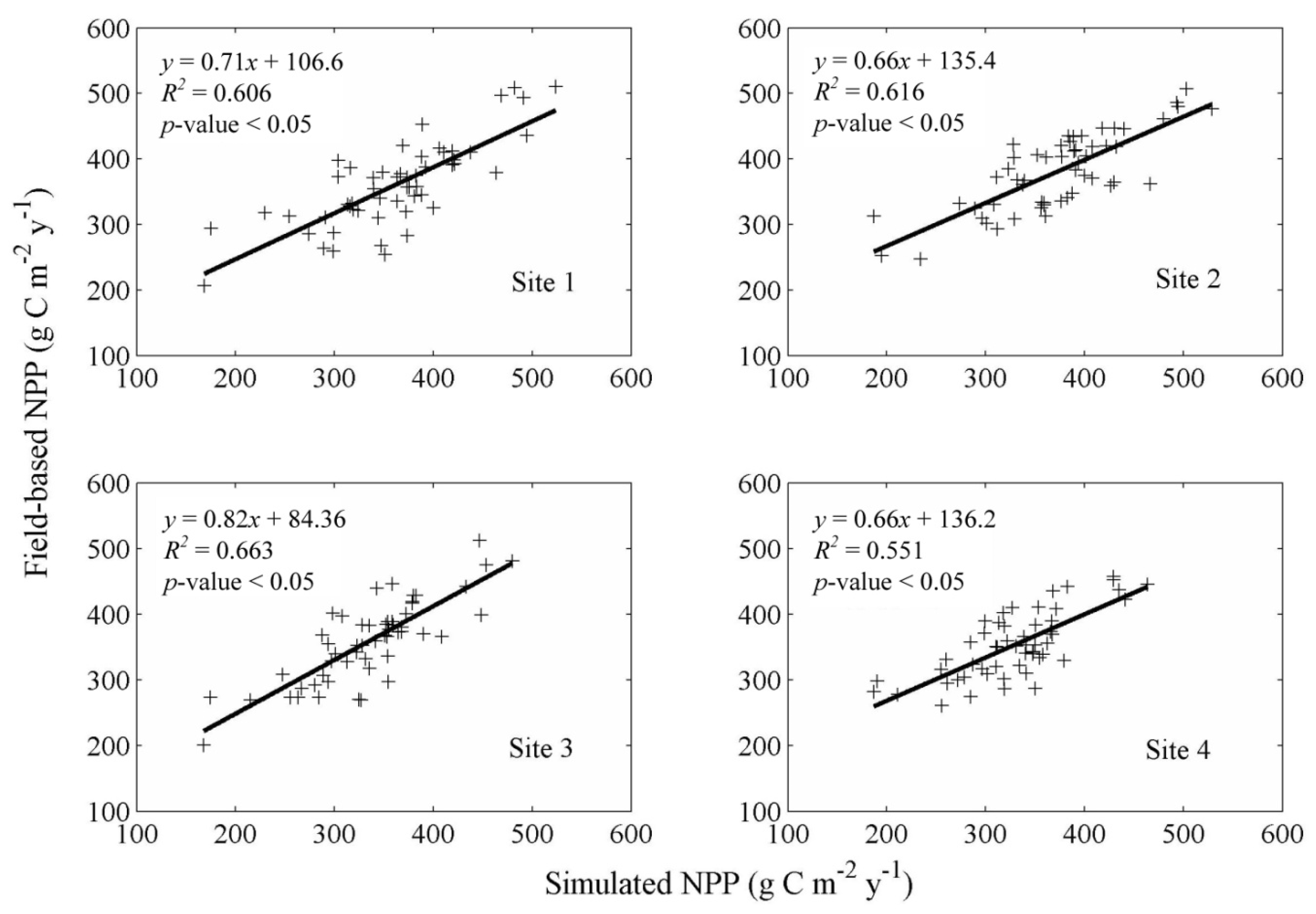
2.3. Field-Based Estimation of Annual NPP

By using the field survey data, biomass value for a whole tree could be calculated fromDBH (cm) and H (m) following the allometric relationship ofindividual P. crassifolia [22]. The allometric equation used was as follows:
W = 0.2561 ( D B H 2 H ) 0.7425
where W is the biomass value of a whole tree (kg). The relationship between DBH and H for individual stems was derived at each site using the following equation:
H = a ( D B H ) b
where a and b are regression coefficients. Summary statistics and the values of the a and b parameters for each site are included in Appendix A. Then, in each site, the mean radial growth widths on different DBH classes were calculated from increment cores of sample trees. Third, according to the DBH classes, all measured trees in the site were divided and given corresponding mean radial growth increment. Finally, based on the Equations (1) and (2) and corresponding mean radial growth increment, annual biomass of individual trees were calculated and extrapolated to the plot level (kg·m−2·year−1) by summing values for individual stems. For comparison with model-predicted NPP values, field-based NPP data were converted to grams of carbon per square meter per year (g·C·m−2·year−1), where 1 g carbon is equivalent to 1.907 g oven-dry organic matter of P. crassifolia [21].

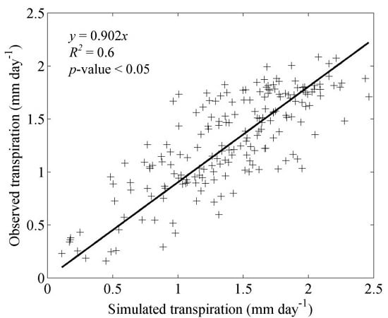
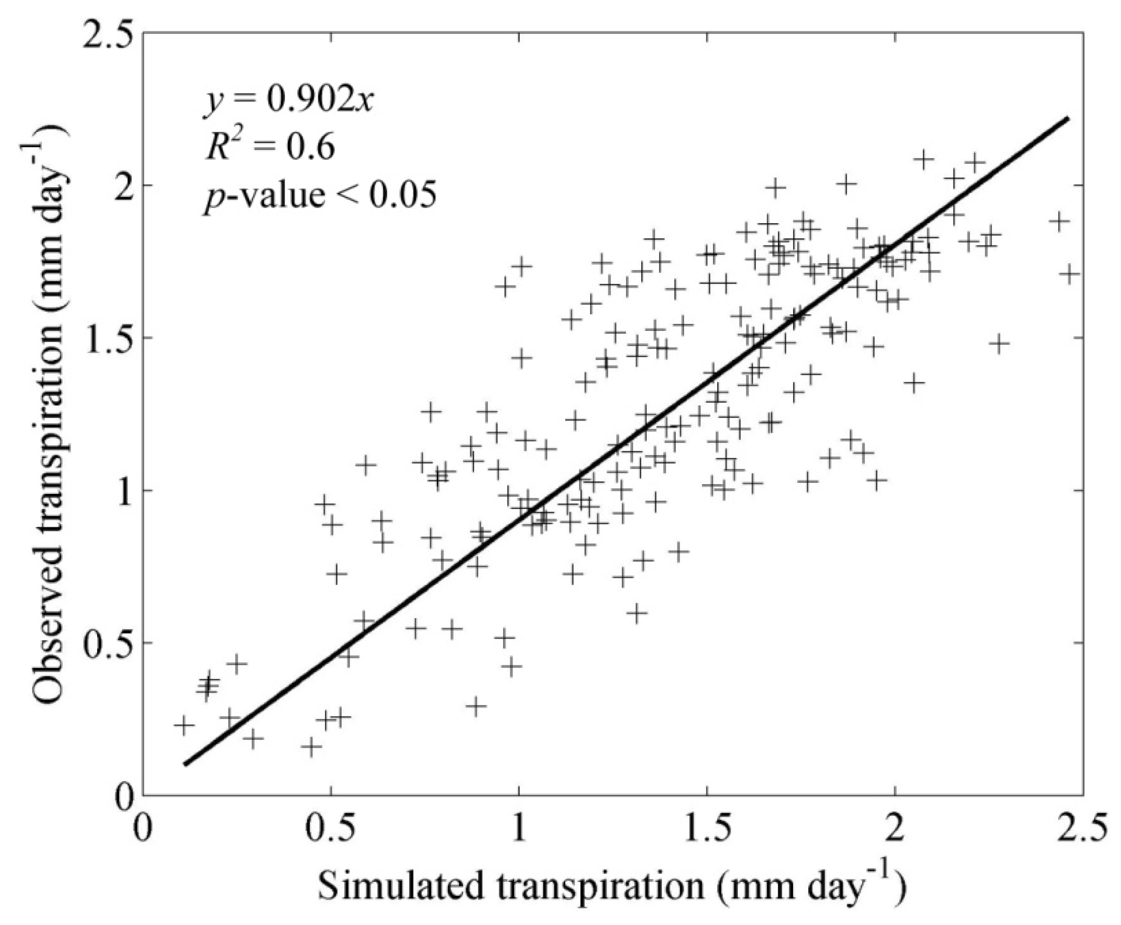
2.4. Calculation of Daily Transpiration

Through temperature differential (ΔT) in tree stem between the paired headed and unheated probes measured by sap flow sensors, individual tree sap flow density (Js, cm3·cm−2·min−1) can be calculated using the following equation [27]:
J s = 0.714 × ( Δ T max Δ T ( Δ T R 1 + Δ T R 2 ) / 2 Δ T ( Δ T R 1 + Δ T R 2 ) / 2 ) 1.23
where ΔTR1 and ΔTR2 are both the temperature differential in tree stem between two unheated probes to improve the ΔT value. ΔTmax is ΔT value in cases where the tree is saturated, i.e., the radial tree trunk does not increase, and air humidity is 100%, with transpiration approaching zero. The transpiration (Es, mm·h−1) for P. crassifolia at stand scale could be calculated by scaling up the individual-level Js using the following equation:
E s = 0.06 × J m e a n × A s tan d
where Astand (cm2·m−2) is the sapwood area per unit area of the total stand. Jmean is the mean Js of sample trees, and is calculated as follows:
J m e a n = i = 1 n J s i × A s i / i = 1 n A s i
where Jsi and Asi are sap flow density and sapwood area on tree i, respectively, and n is number of sampling trees. Based on the relationship between DBH (0.1 cm) and sapwood area (As, mm2) of P. crassifolia [23], As of each P. crassifolia individual at Site3 was calculated using the following equation:
A s = 12655.61 × e D B H 226.72 13306.78
Then, transpiration with one-hour interval was summed to daily value (mm d−1) for validating predicted amount of daily transpiration from the Biome-BGC model.

2.5. Model Description

The Biome-BGC model is often used to estimate contents and fluxes of carbon, nitrogen, and water into and out of an ecosystem [28]. The most recent version of Biome-BGC [29] has been extended to include different biomes (i.e., evergreen needle leaf, evergreen broadleaf, deciduous broadleaf, shrub, and grass) and is suitable for applications for which the user wishes to evaluate drivers of vegetation growth and decay. Mechanisms that control carbon and water fluxes in the Biome-BGC model have been described in detail in Wang et al. [28] and Golinkoff [29]. In general, the model includes a representation of the response of intercellular CO2 concentrations with rising atmospheric concentrations which results in a corresponding increase in plant NPP. In addition, the increase in intercellular CO2 leads to a reduction in stomatal conductance which translates to a reduction in transpiration rates.
Moreover, utilization of the model for predicting flux changes under future climate and atmospheric CO2 concentration scenarios has been described [7,8]. First, model outputs under current climate and atmospheric CO2 concentration conditions should be validated using the field-based data. Second, if simulated values are close to field-based measurements, then the model can be used to simulate this flux under future climate and atmospheric CO2 concentration scenarios through climate change and CO2 control options in the initialization file of the model [7,8].

2.6. Model Parameterization

The Biome-BGC model requires numerous parameters, including site-specific parameters, vegetation ecophysiological characteristics, daily meteorological data, and atmospheric CO2 concentrations. Site-specific parameters are listed in Table 2. The ecophysiological characteristics of P. crassifolia for running Biome-BGC were parameterized based uponaprevious study [17]. A detailed list of the parameters is provided in Appendix B.
Daily meteorological data, including maximum and minimum temperature, precipitation, solar radiation, vapor pressure deficit, and day length, were generated by a modified MTCLIM. The original MTCLIM was modified [30] with multiple weather stations in the Qilian Mountains, which can reduce estimated deviation caused by the distance between weather station and study site. Meteorological records (daily maximum and minimum air temperature, daily precipitation, and average wind direction of the rainy season for 1960–2014), driving the modified MTCLIM were obtained from 19 national weather stations in and around the Qilian Mountains (http://cdc.cma.gov.cn).
No record is available on the atmospheric CO2 concentrations in the Qilian Mountains. Thus, data for 1960–2013 were obtained from direct observations at the Mauna Loa Observatory and were adopted in the simulations [31].

2.7. Climate and CO2 Scenarios

Future climate data under four RCP scenarios were obtained from WorldClim dataset (http://www.worldclim.org/). The four RCPs are known as RCP2.6 [32], RCP4.5 [33,34,35], RCP6.0 [36,37], and RCP8.5 [38], with the label indicating the approximate radiative force in watts per square meter exerted by greenhouse gas and aerosol burden in 2100.Climate data used in this study were downscaled from a general circulation model (BCC-CSM1-1) to a resolution of 1 km × 1 km. Furthermore, the downscaled framework employed in WorldClim is the delta method, which belongs to the statistical downscaling way. The climate period evaluated in this study was the late part of the current century (2061–2080 period), at which time the projected climate represents a substantial change relative to the 1986–2005 period [3]. Furthermore, current climate data (1950–2000) interpolated from the observed data around the world were obtained from the WorldClim dataset. By considering the difference between the current and future climate data, we obtained the change values of temperature and precipitation under the four RCPs. The future CO2 dataunder the four RCP scenarios were acquired from RCP database [39]. For the purposes of this study, the level of climate change and CO2 change were set as constants in the Biome-BGC model using the climate change and CO2 control options in the initialization file of the model.
To completely analyzethe effects of climate and atmospheric CO2 concentration changes on the WUE of P. crassifolia forests, we set two schemes as follows. One scheme presented WUE variations under different RCP scenarios (Table 3), and the other scheme presented WUE responses to different combinations of future climate and atmospheric CO2 concentration changes (Table 4). In this study, climate and CO2 concentrations of 1960–2000 were set as the baseline (current scenario), and the change values in the Table 3 and Table 4 would be the constants to drive the Biome-BGC model based on the current scenario.

2.8. Model Simulation

In cases where starting conditions for the model’s state variables are unavailable, initial conditions may be established using a spin-up run. In a spin-up run, reference or historical climate data are used to drive the model to allow it to reach a steady state condition with respect to ecosystem C and N pools. In this study, 55-year climate records would circularly run the model until the C and N pools were both equalized. By using the endpoint of the spin-up run as the initial condition, the model first reconstructed WUE series for the last 55 years (using the observed climatic data and atmospheric CO2 concentrations during the1960–2014 period) to provide validations. Then, to assess the impact of climate and atmospheric CO2 concentration changes on WUE of P. crassifolia forests, the model was run with each scenario in Table 3 and Table 4 for each site. Prior to evaluating the WUE variations under each scenario, NPP and transpiration variations were calculated first under the scenarios in Table 3 and Table 4.

3. Results

3.1. Model Validation

When run using climate data and atmospheric CO2 concentrations from 1960–2014, model predictions of annual NPP were consistent with observations of NPP derived from the field measurements of radial increments in each site (Figure 2). Simulated daily transpiration rates in 2013 and 2014 were also strongly correlated with field-measured rates during the same time period in Site3 (Figure 3).

3.2. Responses of NPP, Transpiration, and WUE to RCP Scenarios

With the simulated NPP values under climate data and atmospheric CO2 concentrations of 1960–2000 (current scenario) as a baseline for comparison, predicted NPP of P. crassifolia forests under RCP scenarios (Table 3) increased by at least 23% (Table 5). NPP changes exhibited some differences not only among RCP scenarios, but also among different sites. NPP increased with increasing emission intensity (from RCP2.6 to RCP8.5) at each site, and average increments under RCP2.6, 4.5/6.0, and 8.5 scenarios were 26.3%, 42.5%/47%, and 65.9%, respectively. Moreover, NPP increased with rising site elevation; average increments were 40.3% for Site1, 42.3% for Site2, 49% for Site3, and 50.1% for Site4.
Compared to the current scenario, predicted transpiration of P. crassifolia forests decreased under each RCP scenario (Table 6). Transpiration changes exhibited some differences not only among RCP scenarios, but also among different sites. Transpiration decreased with increasing emission intensity (from RCP2.6 to RCP8.5) at each site, and average decrements under RCP2.6, 4.5/6.0, and 8.5 scenarios were 2.6%, 7.2%/7.7%, and 10.2%, respectively. Moreover, transpiration decreased with rising site elevation, except atSite2; average decrements were 6.4% for Site1, 7.8% for Site2, 6.6 % for Site3, and 6.9% for Site4.
Compared to the current scenario, predicted WUE of P. crassifolia forests under RCP scenarios (Table 3) increased by at least 26.2% (Table 7). The WUE changes also exhibited some differences not only among RCP scenarios but also among different sites. The WUE increased with increasing emission intensity (from RCP2.6 to RCP8.5) at each site, and average increments under RCP2.6, 4.5/6.0, and 8.5 scenarios were 29.9%, 53.9%/59.5%, and 85.1%, respectively. Moreover, the WUE increased with rising site elevation; the average increments were 50.5% for Site1, 55.1% for Site2, 60.4% for Site3, and 62.4% for Site4.

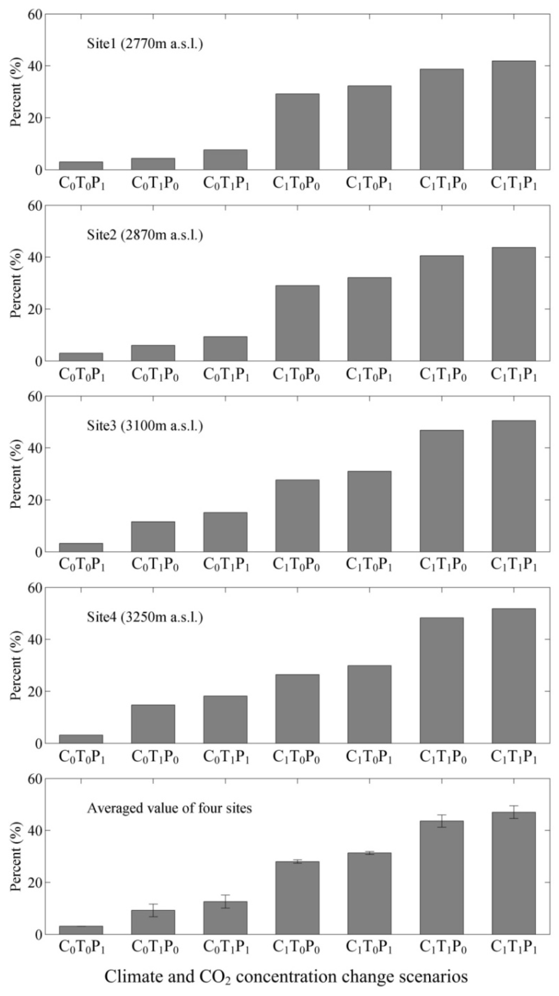
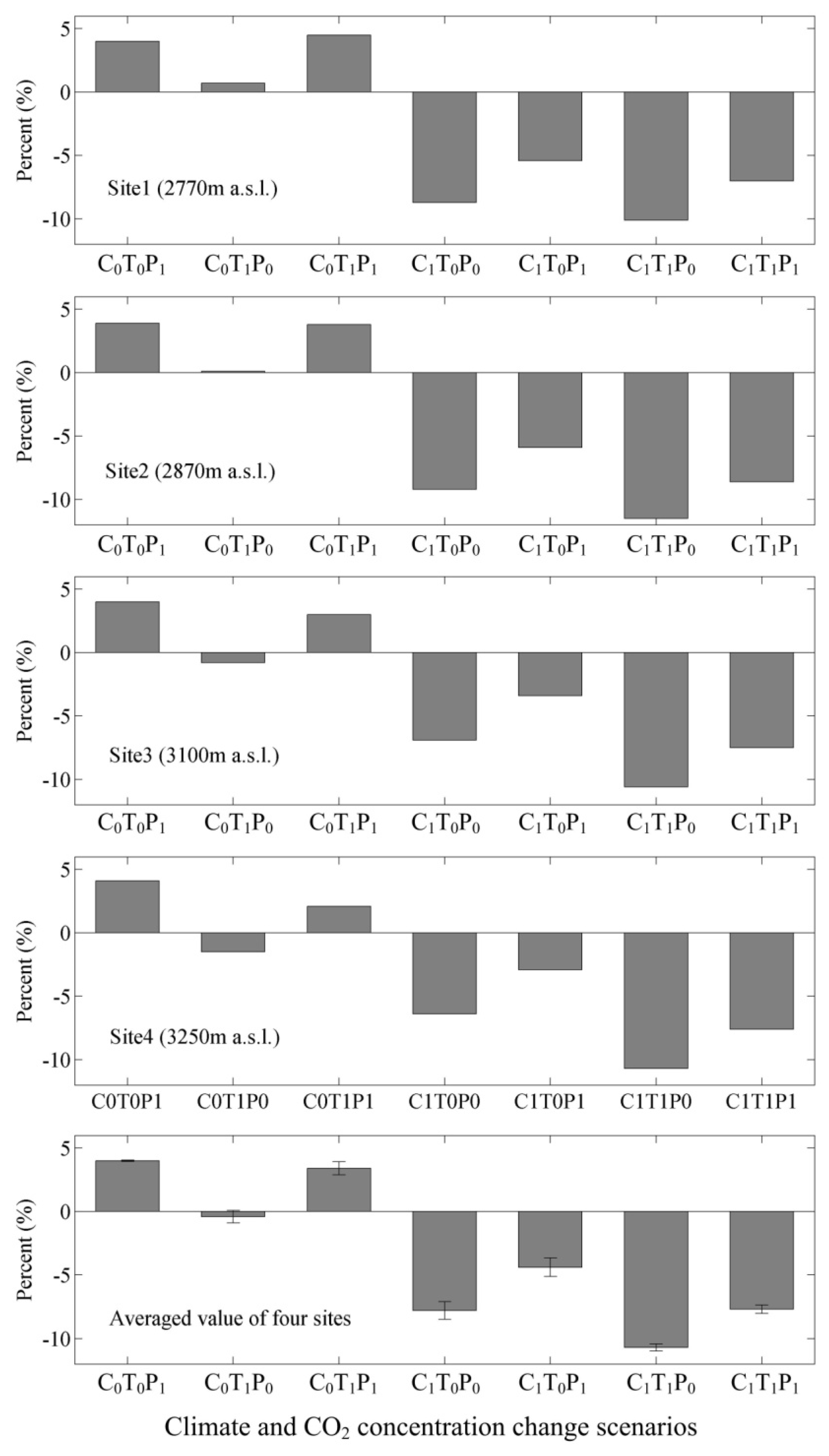
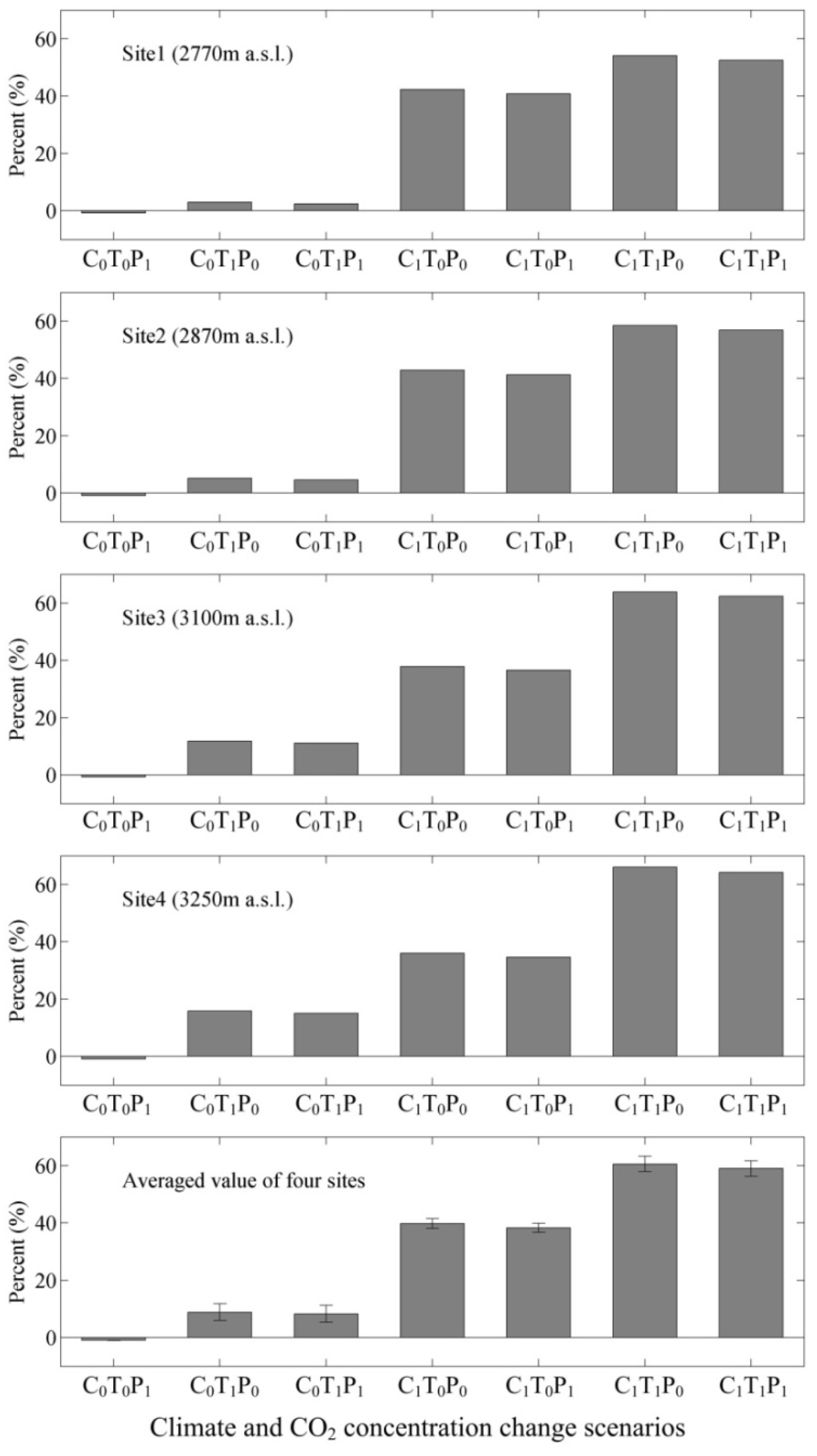
3.3. Responses of NPP, Transpiration, and WUE to Changes in Climate and Atmospheric CO2 Concentrations

With simulated values under C0T0P0 scenario (climate data of 1960–2000 and 340 ppm CO2 concentration) as a baseline for comparison, predicted NPP of P. crassifolia forests increased by about 3.1% when precipitation increases alone were considered (under the C0T0P1 scenario). The NPP increments were essentially consistent among the sites (Figure 4). The effects of the temperature increases alone (under the C0T1P0 scenario) were positive for all of the sites, and average NPP increment was about 9.2%. Furthermore, the NPP increments were not uniform and ranged from 4.3% (for Site1) to 14.7% (for Site4). Besides, the NPP increased with rising site elevation (Figure 4). With the changes in both temperature and precipitation (under the C0T1P1 scenario), NPP increased by about 12.6%, ranging from 7.6% (for Site1) to 18.2% (for Site4). In contrast to climate change results, simulated results indicated that NPP showed a relatively intense response to atmospheric CO2 concentrations alone (under C1T0P0 scenario); NPP increased by about 28%, and NPP increments were basically consistent among the sites. Along with the changes in both precipitation and atmospheric CO2 concentrations (under C1T0P1 scenario), NPP increased by about 31.3%, and NPP increments were nearly consistent among the sites. Variations in both temperature and atmospheric CO2 concentrations (under C1T1P0 scenario) increased NPP by about 43.6% (ranging from 38.7% for Site1 to 48.3% for Site4). When all climate and atmospheric CO2 concentration alterations were considered (under C1T1P1 scenario), NPP increased by about 47% (ranging from 41.9% for Site1 to 51.8% for Site4) (Figure 4).
Compared with the C0T0P0 scenario, predicted transpiration of P. crassifolia forests increased by about 4% when precipitation increases alone were considered (under C0T0P1 scenario). Transpiration increments were essentially consistent among the sites (Figure 5). Effects of temperature increases alone (under C0T1P0 scenario) were slight for the sites, and average transpiration decrement was about 0.4%.With the changes in both temperature and precipitation (under C0T1P1 scenario), transpiration increased by about 3.4%, ranging from 4.5% (for Site1) to 2.1% (for Site4). In contrast to the climate change results, the simulated results indicated that transpiration showed a relatively intense response to atmospheric CO2 concentrations alone (under C1T0P0 scenario); transpiration decreased by about 7.8%, and transpiration decrements were basically consistent among the sites. Along with the changes in both precipitation and atmospheric CO2 concentrations (under C1T0P1 scenario), transpiration decreased by about 4.4%. Variations in both temperature and atmospheric CO2 concentrations (under C1T1P0 scenario) decreased transpiration by about 10.7%. When all climate and atmospheric CO2 concentration alterations were considered (under C1T1P1 scenario), transpiration decreased by about 7.7% (Figure 5).
Compared with the C0T0P0 scenario, the predicted WUE of P. crassifolia forests decreased by about 0.9% when precipitation increases alone were considered (under C0T0P1 scenario). The WUE decrements were essentially consistent among the sites (Figure 6). Effects of temperature increases alone (under C0T1P0 scenario) were positive for all of the sites, and average WUE increment was about 8.9%. Furthermore, the WUE increments were not uniform and ranged from 3% (for Site1) to 15.8% (for Site4). Besides, the WUE increased with rising site elevation (Figure 6). With changes in both temperature and precipitation (under C0T1P1 scenario), WUE increased by about 8.3%, ranging from 2.4% (for Site1) to 15% (for Site4). In contrast to the climate change results, the simulated results indicated that WUE showed a relatively intense response to atmospheric CO2 concentrations alone (under C1T0P0 scenario); WUE increased by about 39.8%, and WUE increments were basically consistent among the sites. Along with changes in both precipitation and atmospheric CO2 concentrations (under C1T0P1 scenario), WUE increased by about 38.3%, and WUE increments were nearly consistent among the sites. Variations in both temperature and atmospheric CO2 concentrations (under C1T1P0 scenario) increased WUE by about 60.6% (ranging from 54.1% for Site1 to 66% for Site4). When all climate and atmospheric CO2 concentration alterations were considered (under C1T1P1 scenario), WUE increased by about 59% (ranging from 52.5% for Site1 to 64.2% for Site4) (Figure 6).

4. Discussion

4.1. Model Validation

In a previous study, we used Biome-BGC to model the stem volume size of P. crassifolia forests at other sites based on simulated stem carbon [17]. The model presented a favorable performance in simulating stem carbon of P. crassifolia forests. However, to ensure that the model also performs well in simulating NPP and transpiration of P. crassifolia forests, the model was further tested in this study. Using climate data and atmospheric CO2 concentrations of 1960–2014, estimations of annual NPP and daily transpiration from Biome-BGC were close to field-based measurements at sites (Figure 2 and Figure 3). Combining the validations in previous and current studies, this study suggested that the Biome-BGC model was suitable for estimating annual NPP and transpiration of P. crassifolia forest under current climate and CO2 concentration conditions. Thus, the validation exercise provided a level of confidence in the model capability to project the impacts of climate change and changing atmospheric CO2 concentrations on NPP and transpiration of P. crassifolia forest at each site under future climatic conditions and CO2 concentration, as suggested by Nunes et al. [8] and Su et al. [7].

4.2. WUE Variations under RCP Scenarios

Different radiative forcing levels and their continuous time for each RCP scenario cause varying future climate and CO2 concentration trends around the world [40]. In general, a higher radiative forcing level generates greater increases in future temperature and atmospheric CO2 concentrations; the increase in precipitation does not differ significantly among RCP scenarios in China [40,41]. In this study, CO2 concentration and increases in temperature and precipitation under different RCP scenarios at the four sites almost conformed to the findings of Xu and Xu [41].
In this study, responses of predicted WUE to different RCP scenarios were positive in all of the sites, and the increases in WUE differed under various RCP scenarios (Table 7). Under each RCP scenario, increases in temperature, precipitation, and CO2 concentration enhanced NPP and decreased transpiration at each site (Table 5 and Table 6), which resulted in WUE increment.
To date, very few studies have examined the response of forest WUE to the RCP scenarios at ecosystem scale. The results in this study indicate that differences in radiative forcing level in RCPs could be responsible for different WUE increases. Furthermore, by comparing WUE differences among RCP scenarios, greater increases in temperature, precipitation, and CO2 concentration generate greater increments in WUE.

4.3. Climate Change Versus WUE Variations

In the Biome-BGC model, elevated temperatures may increase NPP through metabolically enhanced photosynthesis and by prolonging the growing season, as well as increasing nutrient availability through higher rates of decomposition [29,42]. Elevated temperatures, however, may also decrease NPP by decreasing soil moisture and enhancing plant respiration [26]. Thus, the sole increase in temperature may not only raise WUE by increasing NPP, but also decrease WUE by enhancing plant transpiration. In this study, because the temperature effect on NPP increase was much more than that on transpiration increase under the C0T1P0 scenario (Figure 4 and Figure 5), responses of predicted WUE to this scenario were positive at all sites (Figure 6). These results suggested that the positive effects of temperature increase were greater than the negative effects on WUE of P. crassifolia forests. However, the effect of increasing temperature on NPP is different from the study by Chiesi et al. [9], who found that elevated temperature decreased NPP in deciduous oak and mountain conifer ecosystem. This difference may be related to the fact that the P. crassifolia forest is a temperate forest, for which increased temperature is generally associated with increased NPP [8]. Besides, the P. crassifolia NPP increased with rising site elevation (Figure 4), which implies that temperature really is a significant factor affecting temperate forest NPP, especially in the high-elevation regions.
In the Biome-BGC model, the increasing precipitation could directly improve water availability for plants, and then plant NPP and transpiration would increase [7,29,42]. Therefore, the response of plant WUE to the increasing precipitation is an integrated process [43]. In this study, because precipitation effect on increasing the transpiration was slightly more than that on the NPP increase under C0T0P1 scenario (Figure 4 and Figure 5), the responses of predicted WUE to this scenario were negative at all sites (Figure 6). These results suggested that the negative effects of precipitation increase were greater than the positive effects on WUE of P. crassifolia forests. Moreover, the effects of increasing precipitation on NPP conform to the studies by Su et al. [7], Nunes et al. [8], and Chiesi et al. [9]. However, these effects were smaller than the effects of increasing temperature on NPP at each site (Figure 4). These differences are likely related to the fact that our high-elevation study sites are relatively moist and largely limited by low temperatures. In contrast, the other studies were located in relatively droughty [8,9] or low-elevation [7] regions, in which the effects of increasing precipitation on NPP was very outstanding.
Along with the changes in both temperature and precipitation (under the C0T1P1 scenario), WUE increased at all sites (Figure 6).Keenan and Richardson [44] found that future climate change would affect forest phenology and suggested that this mechanism should be included in the predictive model. In the Biome-BGC model, plant phenology has been described as a function of climatic variables; therefore, WUE estimations under the C0T1P1 scenario were reasonable. Moreover, a combination of temperature and precipitation exhibited strong interactive effects on forest WUE (Figure 4, Figure 5 and Figure 6), which was determined by inner mechanisms of Biome-BGC [29].

4.4. Atmospheric CO2 Concentration Changes versus WUE Variations

In the present study, predicted NPP showed a relatively intense response to atmospheric CO2 concentration increase alone (under C1T0P0 scenario), and about 28% increase in NPP was noted for each site (Figure 4). These results are in agreement with those obtained from free-air-CO2-enrichment (FACE) experiments and scenario simulation studied by: Norby et al. [45], who found that NPP of four different forests increased by about 23% under elevated CO2 (550 ppm); Ainsworth and Long [46], who found a 28% increase in aboveground biomass of trees under elevated CO2 concentration (from 475 to 600 ppm); Smith et al. [47], who reported that the mean effect of CO2 enrichment (580 ppm) on aboveground woody biomass was about 22.3%; and Nunes et al. [8], who found that the NPP of forests were predicted to increase (about 24%) in the future with a CO2 increase. However, it should be pointed out that the CO2 fertilization effect on forest NPP observed in the FACE experiments has been short-lived as other factors soon become limiting, such as low temperature, forest leaf area index (LAI), and nitrogen [48]. Furthermore, these results suggested that responses of P. crassifolia NPP to the atmospheric CO2 concentration are more intense than to the climate change.
Meanwhile, predicted transpiration also showed a relatively intense response under C1T0P0 scenario (Figure 5). In this study, we used 55-year data to drive the model to simulate the forest NPP and transpiration under various scenarios, and in this long time simulation the forest LAI would increase due to rising forest NPP. Thus, the through fall would decrease and then the soil water used for transpiration would decrease. Finally, predicted transpiration decreased by about 7.8% for each site under the C1T0P0 scenario. Furthermore, compared to this scenario, the decrement of transpiration is smaller under the C1T0P1 scenario at about 4.4%, which is due to there being more soil water used for transpiration. Therefore, increased NPP and decreased transpiration resulted in a large increment (about 39.8%) in WUE under C1T0P0 scenario (Figure 6).
Compared to the effects of climate changes (under C0T1P0, C0T0P1, and C0T1P1 scenarios) on P. crassifolia WUE, effect of atmospheric CO2 concentration is more intense (Figure 6). This inference is different from the study from Sang and Su [42], who found that the precipitation is the most sensitive factor affecting the WUE of P. schrenkiana forest (site elevations ≤2440 m). This difference may be caused by the fact that forest carbon assimilation is more sensitive to the CO2 concentration in relatively higher elevation regions [49,50], like the forest sites (2770–3250 m) in this study.
Moreover, other studies found that the increase in atmospheric CO2 concentration has not improved tree growth [13] or prevented forest NPP accumulation over a long time [51]. These findings implied that the change in atmospheric CO2 concentration could lead to the change of forest adaptability to surrounding environment [52]. For example, change in atmospheric CO2 concentration could lead to a change in stomatal conductance [53], which would affect photosynthesis and transpiration rates. Thus, atmospheric CO2 concentration effect on forest WUE is dual. To date, negative effects of atmospheric CO2 concentration have not been described in Biome-BGC. Therefore, description of this influencing mechanism in the model is needed.

4.5. Climate and CO2 Concentration Changes versus WUE Variations

In the study sites, simultaneous increase in temperature and CO2 concentrations led to a remarkable increment in P. crassifolia forest WUE (ranging from 54.1% to 66% under C1T1P0 scenario), and their combination exhibited strong interactive effects on forest WUE. However, WUE increases under C1T1P1 scenario were slightly lower than those under C1T1P0 scenario, which was due to the fact that the sole increase in precipitation (under C0T0P1 scenario) could result in a negative effect on forest WUE (Figure 6). Moreover, the response of forest WUE to future global changes (under C1T1P1 scenario) was more intense at high elevations than at low elevations. Furthermore, compared to the temperature and precipitation, the CO2 concentration was the main factor controlling forest WUE variations in high elevation regions (Figure 6).
In this study, due to the fact that it is difficult to obtain downscaled future daily climate data, we set the change values of climate and CO2 concentration as the constants to analyze the effects of future climate and CO2 concentration changes on the forest NPP, transpiration, and WUE. Therefore, the continuous forest system responses cannot be obtained from the study. Besides, the Biome-BGC model is a static vegetation model and cannot capture the dynamic forest processes, like regeneration, competition, and succession. These processes could undertake some changes in forest NPP and LAI [54]. An alternative way for studying the responses of forest ecosystem to future global change is the utilization of dynamic vegetation model, like the LPJ-GUESS model [55]. In addition, the continuous monthly climate data for driving the model could be obtained from general circulation models through a statistical downscaling technique [56].

5. Conclusions

The Biome-BGC estimates showed good agreement with independent field-based NPP and transpiration values at the sites of P. crassifolia forests in the Qilian Mountains of Northwest China. Therefore, the model can be used to study forest WUE responses to global changes. Under different RCP scenarios, model simulations showed that greater increases in temperature, precipitation, and CO2 concentration would cause more increases in P. crassifolia forest WUE.
At the study sites, the effect of atmospheric CO2 concentration is more significant than that of climate change. An increase in both temperature and atmospheric CO2 concentration led to a remarkable increase in P. crassifolia forest WUE, and their combination had strong interactive effects on WUE. Moreover, WUE response to global changes in high elevations was more intense than that in low elevations, and the CO2 concentration was the main factor controlling forest WUE variations. These valuable predictions could be helpful in understanding how forest ecosystems respond to simultaneous or independent changes in climate and atmospheric CO2 concentrations.

Acknowledgments

This work was supported by the Western Light Program of Chinese Academy of Sciences (No. XAB2015B07), the Ph.D. Start-Up fund of Northwest A & F University (No. 2452015343), and National Natural Science Foundation of China (No. 91025015).The authors wish to thank two anonymous reviewers for their constructive suggestions to improve the quality of this article.

Author Contributions

Shouzhang Peng and Yang Cao conceived and designed the experiments; Shouzhang Peng performed the experiments; Shouzhang Peng and Yunming Chen analyzed the data; Shouzhang Peng, Yunming Chen and Yang Cao wrote the paper.

Conflicts of Interest

The authors declare no conflict of interest.

Appendix A

Table A1. Regression coefficients and statistical indicators of Equation (2) at each site.
SitesabR2p-Value
Site10.9620.9100.902<0.001
Site21.1390.8490.943<0.001
Site31.1190.8530.896<0.001
Site40.6980.9370.921<0.001

Appendix B

Table B1. Ecophysiological parameters of P. crassifolia forest for running Biome-BGC model.
No.Parameter DescriptionValueUnit a
1Transfer growth period as a fraction of growing season0.3DIM
2Litterfall as a fraction of growing season0.3DIM
3Annual leaf and fine root turnover fraction0.25year−1
4Annual live wood turnover fraction0.7year−1
5Annual whole-plant mortality fraction0.005year−1
6Annual fire mortality fraction0.005year−1
7(Allocation) new fine root C: new leaf C1.0ratio
8(Allocation) new stem C: new leaf C2.2ratio
9(Allocation) new live wood C: new total wood C0.1ratio
10(Allocation) new root C: new stem C0.3ratio
11(Allocation) current growth proportion0.5DIM
12C:N of leaves40.2kg C/kg N
13C:N of leaf litter, after retranslocation94.6kg C/kg N
14C:N of fine roots43.5kg C/kg N
15C:N of live wood60.0kg C/kg N
16C:N of dead wood720.0kg C/kg N
17Leaf litter labile proportion0.32DIM
18Leaf litter cellulose proportion0.44DIM
19Leaf litter lignin proportion0.24DIM
20Fine root labile proportion0.3DIM
21Fine root cellulose proportion0.45DIM
22Fine root lignin proportion0.25DIM
23Dead wood cellulose proportion0.76DIM
24Dead wood lignin proportion0.24DIM
25Canopy water interception coefficient0.0411/LAI/d
26Canopy light extinction coefficient0.5DIM
27All-sided to projected leaf area ratio2.6DIM
28Canopy average specific leaf area (projected area basis)9.3m2/kg C
29Ratio of shaded SLA: sunlit SLA2.0DIM
30Fraction of leaf N in Rubisco0.04DIM
31Maximum stomatal conductance (projected area basis)0.003m/s
32Cuticular conductance (projected area basis)0.00001m/s
33Boundary layer conductance (projected area basis)0.08m/s
34Leaf water potential: start of conductance reduction−0.6M Pa
35Leaf water potential: complete conductance reduction−2.3M Pa
36Vapor pressure deficit: start of conductance reduction930.0Pa
37Vapor pressure deficit: complete conductance reduction4100.0Pa
a DIM: dimensionless.

References

  1. IPCC 2013. Climate Change 2013: The Physical Science Basis. In Contribution of Working Group I to the Fifth Assessment Report of the Intergovernmental Panel on Climate Change; Stocker, T.F., Qin, D., Plattner, G.-K., Tignor, M., Allen, S.K., Boschung, J., Nauels, A., Xia, Y., Bex, V., Midgley, P.M., Eds.; Cambridge University Press: Cambridge, UK; New York, NY, USA, 2013; p. 1535. [Google Scholar]
  2. Xu, Z.; Zhao, C.; Feng, Z.; Zhang, F.; Sher, H.; Wang, C.; Peng, H.; Wang, Y.; Zhao, Y.; Wang, Y. Estimating realized and potential carbon storage benefits from reforestation and afforestation under climate change: A case study of the Qinghai spruce forests in the Qilian Mountains, northwestern China. Mitig. Adapt. Strateg. Glob. Chang. 2013, 18, 1257–1268. [Google Scholar] [CrossRef]
  3. IPCC. Synthesis Report. Contribution of Working Groups I, II and III to the Fifth Assessment Report of the Intergovernmental Panel on Climate Change; Core Writing Team; Pachauri, R.K., Meyer, L.A., Eds.; IPCC: Geneva, Switzerland, 2014; p. 151. [Google Scholar]
  4. Grimm, N.B.; Chapin, F.S., III; Bierwagen, B.; Gonzalez, P.; Groffman, P.M.; Luo, Y.; Melton, F.; Nadelhoffer, K.; Pairis, A.; Raymond, P.A. The impacts of climate change on ecosystem structure and function. Front. Ecol. Environ. 2013, 11, 474–482. [Google Scholar] [CrossRef]
  5. Friend, A.D.; Lucht, W.; Rademacher, T.T.; Keribin, R.; Betts, R.; Cadule, P.; Ciais, P.; Clark, D.B.; Dankers, R.; Falloon, P.D. Carbon residence time dominates uncertainty in terrestrial vegetation responses to future climate and atmospheric CO2. Proc. Natl. Acad. Sci. USA 2014, 111, 3280–3285. [Google Scholar] [CrossRef] [PubMed]
  6. Dixon, R.K.; Brown, S.; Houghton, R.A.; Solomon, A.M.; Trexler, M.C.; Wisniewski, J. Carbon pools and flux of global forest ecosystems. Science 1994, 263, 185–190. [Google Scholar] [CrossRef] [PubMed]
  7. Su, H.; Sang, W.; Wang, Y.; Ma, K. Simulating Picea schrenkiana forest productivity under climatic changes and atmospheric CO2 increase in Tianshan Mountains, Xinjiang Autonomous Region, China. For. Ecol. Manag. 2007, 246, 273–284. [Google Scholar] [CrossRef]
  8. Nunes, L.; Gower, S.T.; Peckham, S.D.; Magalhães, M.; Lopes, D.; Rego, F.C. Estimation of productivity in pine and oak forests in northern Portugal using Biome-BGC. Forestry 2015, 88, 200–212. [Google Scholar] [CrossRef]
  9. Chiesi, M.; Moriondo, M.; Maselli, F.; Gardin, L.; Fibbi, L.; Bindi, M.; Running, S.W. Simulation of Mediterranean forest carbon pools under expected environmental scenarios. Can. J. For. Res. 2010, 40, 850–860. [Google Scholar] [CrossRef]
  10. Ågren, G.I.; Andersson, F.O. Terrestrial Ecosystem Ecology: Principles and Applications; University Press: Cambridge, UK, 2011. [Google Scholar]
  11. Bonan, G. Ecological Climatology: Concepts and Applications; Cambridge University Press: Cambridge, UK, 2015. [Google Scholar]
  12. Niu, S.; Xing, X.; Zhang, Z.; Xia, J.; Zhou, X.; Song, B.; Li, L.; Wan, S. Water-use efficiency in response to climate change: from leaf to ecosystem in a temperate steppe. Glob. Chang. Biol. 2011, 17, 1073–1082. [Google Scholar] [CrossRef]
  13. Silva, L.C.; Anand, M. Probing for the influence of atmospheric CO2 and climate change on forest ecosystems across biomes. Glob. Ecol. Biogeogr. 2013, 22, 83–92. [Google Scholar] [CrossRef]
  14. Battipaglia, G.; Saurer, M.; Cherubini, P.; Calfapietra, C.; McCarthy, H.R.; Norby, R.J.; Francesca Cotrufo, M. Elevated CO2 increases tree-level intrinsic water use efficiency: Insights from carbon and oxygen isotope analyses in tree rings across three forest FACE sites. New Phytol. 2013, 197, 544–554. [Google Scholar] [CrossRef] [PubMed]
  15. Rötzer, T.; Liao, Y.; Goergen, K.; Schüler, G.; Pretzsch, H. Modelling the impact of climate change on the productivity and water-use efficiency of a central European beech forest. Clim. Res. 2013, 58, 81–95. [Google Scholar] [CrossRef]
  16. Xie, J.; Chen, J.; Sun, G.; Zha, T.; Yang, B.; Chu, H.; Liu, J.; Wan, S.; Zhou, C.; Ma, H. Ten-year variability in ecosystem water use efficiency in an oak-dominated temperate forest under a warming climate. Agric. For. Meteorol. 2016, 218, 209–217. [Google Scholar] [CrossRef]
  17. Peng, S.Z.; Zhao, C.Y.; Xu, Z.L. Modeling stem volume growth of Qinghai spruce (Picea crassifolia Kom.) in Qilian Mountains of Northwest China. Scand. J. For. Res. 2015, 30, 449–457. [Google Scholar]
  18. Tian, F.; Zhao, C.; Feng, Z.-D. Simulating evapotranspiration of Qinghai spruce (Picea crassifolia) forest in the Qilian Mountains, northwestern China. J. Arid Environ. 2011, 75, 648–655. [Google Scholar] [CrossRef]
  19. Zhao, C.; Nan, Z.; Cheng, G.; Zhang, J.; Feng, Z. GIS-assisted modelling of the spatial distribution of Qinghai spruce (Picea crassifolia) in the Qilian Mountains, northwestern China based on biophysical parameters. Ecol. Model. 2006, 191, 487–500. [Google Scholar] [CrossRef]
  20. Liu, X.C. Picea Crassifolia; Lanzhou University Press: Lanzhou, China, 1992. (In Chinese) [Google Scholar]
  21. Wang, J.Y.; Che, K.J.; Rong, J.Z. A study on carbon balance of picea crassifolia in Qilian Mountains. J. Northwest For. Coll. 2000, 15, 9–14. (In Chinese) [Google Scholar]
  22. Wang, J.Y.; Che, K.J.; Fu, H.E.; Chang, X.X.; Song, C.F.; He, H.Y. Study on biomass of water conservation forest on north slope of Qilian Mountains. J. Fujian Coll. For. 1998, 18, 319–323. (In Chinese) [Google Scholar]
  23. Chang, X.; Zhao, W.; Liu, H.; Wei, X.; Liu, B.; He, Z. Qinghai spruce (Picea crassifolia) forest transpiration and canopy conductance in the upper Heihe River Basin of arid northwestern China. Agric. For. Meteorol. 2014, 198, 209–220. [Google Scholar] [CrossRef]
  24. Chang, X.; Zhao, W.; He, Z. Radial pattern of sap flow and response to microclimate and soil moisture in Qinghai spruce (Picea crassifolia) in the upper Heihe River Basin of arid northwestern China. Agric. For. Meteorol. 2014, 187, 14–21. [Google Scholar] [CrossRef]
  25. Wang, W.; Liu, X.; An, W.; Xu, G.; Zeng, X. Increased intrinsic water-use efficiency during a period with persistent decreased tree radial growth in northwestern China: Causes and implications. For. Ecol. Manag. 2012, 275, 14–22. [Google Scholar] [CrossRef]
  26. Thornton, P.; Law, B.; Gholz, H.L.; Clark, K.L.; Falge, E.; Ellsworth, D.; Goldstein, A.; Monson, R.; Hollinger, D.; Falk, M. Modeling and measuring the effects of disturbance history and climate on carbon and water budgets in evergreen needleleaf forests. Agric. For. Meteorol. 2002, 113, 185–222. [Google Scholar] [CrossRef]
  27. Fang, S.; Zhao, C.; Jian, S. Canopy transpiration of Pinus tabulaeformis plantation forest in the Loess Plateau region of China. Environ. Earth Sci. 2016, 75, 1–9. [Google Scholar] [CrossRef]
  28. Wang, Q.; Watanabe, M.; Ouyang, Z. Simulation of water and carbon fluxes using BIOME-BGC model over crops in China. Agric. For. Meteorol. 2005, 131, 209–224. [Google Scholar] [CrossRef]
  29. Golinkoff, J. Biome BGC version 4.2: Theoretical framework of Biome-BGC. Terradynamic Simulation Group Modeling and Monitoring Ecosystem Function at Multiple Scales. Biome-BGC, 2010. Available online: http://www.ntsg.umt.edu/project/biome-bgc (accessed on 4 September 2014).
  30. Peng, S.Z.; Zhao, C.Y.; Wang, X.P.; Xu, Z.L.; Liu, X.M.; Hao, H.; Yang, S.F. Mapping daily temperature and precipitation in the Qilian Mountains of northwest China. J. Mt. Sci. Engl. 2014, 11, 896–905. [Google Scholar] [CrossRef]
  31. Tans, D.P. Monthly Atmospheric CO2 of Mauna Loa Observatory, NOAA/ESRL. Available online: http://www.esrl.noaa.gov/gmd/ccgg/trends (accessed on 5 June 2015).
  32. Van Vuuren, D.P.; Den Elzen, M.G.; Lucas, P.L.; Eickhout, B.; Strengers, B.J.; van Ruijven, B.; Wonink, S.; van Houdt, R. Stabilizing greenhouse gas concentrations at low levels: An assessment of reduction strategies and costs. Clim. Chang. 2007, 81, 119–159. [Google Scholar] [CrossRef]
  33. Clarke, L.; Edmonds, J.; Jacoby, H.; Pitcher, H.; Reilly, J.; Richels, R. Scenarios of greenhouse gas emissions and atmospheric concentrations. In Sub-report 2.1A of Synthesis and Assessment Product 2.1 by the U.S. Climate Change Science Program and the Subcommittee on Global Change Research; US Department of Energy Publications, Department of Energy, Office of Biological & Environmental Research: Washington, DC, USA, 2007; p. 154. [Google Scholar]
  34. Wise, M.; Calvin, K.; Thomson, A.; Clarke, L.; Bond-Lamberty, B.; Sands, R.; Smith, S.J.; Janetos, A.; Edmonds, J. Implications of limiting CO2 concentrations for land use and energy. Science 2009, 324, 1183–1186. [Google Scholar] [CrossRef] [PubMed]
  35. Smith, S.J.; Wigley, T. Multi-gas forcing stabilization with Minicam. Energy J. 2006, 27, 373–391. [Google Scholar] [CrossRef]
  36. Fujino, J.; Nair, R.; Kainuma, M.; Masui, T.; Matsuoka, Y. Multi-gas mitigation analysis on stabilization scenarios using AIM global model. Energy J. 2006, 27, 343–353. [Google Scholar] [CrossRef]
  37. Hijioka, Y.; Matsuoka, Y.; Nishimoto, H.; Masui, T.; Kainuma, M. Global GHG emission scenarios under GHG concentration stabilization targets. J. Glob. Environ. Eng. 2008, 13, 97–108. [Google Scholar]
  38. Riahi, K.; Grübler, A.; Nakicenovic, N. Scenarios of long-term socio-economic and environmental development under climate stabilization. Tech. Forecast. Soc. Chang. 2007, 74, 887–935. [Google Scholar] [CrossRef]
  39. RCP Database (version 2.0). Available online: http://www.iiasa.ac.at/web-apps/tnt/RcpDb (accessed on 1 June 2015).
  40. Van Vuuren, D.P.; Edmonds, J.; Kainuma, M.; Riahi, K.; Thomson, A.; Hibbard, K.; Hurtt, G.C.; Kram, T.; Krey, V.; Lamarque, J.-F. The representative concentration pathways: An overview. Clim. Chang. 2011, 109, 5–31. [Google Scholar] [CrossRef]
  41. Xu, C.H.; Xu, Y. The projection of temperature and precipitation over China under RCP scenarios using a CMIP5 multi-model ensemble. Atmos. Ocean. Sci. Lett. 2012, 5, 527–533. [Google Scholar]
  42. Sang, W.; Su, H. Interannual NPP variation and trend of Picea schrenkiana forests under changing climate conditions in the Tianshan Mountains, Xinjiang, China. Ecol. Res. 2009, 24, 441–452. [Google Scholar] [CrossRef]
  43. Keenan, T.F.; Hollinger, D.Y.; Bohrer, G.; Dragoni, D.; Munger, J.W.; Schmid, H.P.; Richardson, A.D. Increase in forest water-use efficiency as atmospheric carbon dioxide concentrations rise. Nature 2013, 499, 324–327. [Google Scholar] [CrossRef] [PubMed]
  44. Keenan, T.F.; Richardson, A.D. The timing of autumn senescence is affected by the timing of spring phenology: Implications for predictive models. Glob. Chang. Biol. 2015, 21, 2634–2641. [Google Scholar] [CrossRef] [PubMed]
  45. Norby, R.J.; DeLucia, E.H.; Gielen, B.; Calfapietra, C.; Giardina, C.P.; King, J.S.; Ledford, J.; McCarthy, H.R.; Moore, D.J.; Ceulemans, R. Forest response to elevated CO2 is conserved across a broad range of productivity. Proc. Natl. Acad. Sci. USA 2005, 102, 18052–18056. [Google Scholar] [CrossRef] [PubMed]
  46. Ainsworth, E.A.; Long, S.P. What have we learned from 15 years of free-air CO2 enrichment (FACE)? A meta-analytic review of the responses of photosynthesis, canopy properties and plant production to rising CO2. New Phytol. 2005, 165, 351–372. [Google Scholar] [CrossRef] [PubMed]
  47. Smith, A.R.; Lukac, M.; Hood, R.; Healey, J.R.; Miglietta, F.; Godbold, D.L. Elevated CO2 enrichment induces a differential biomass response in a mixed species temperate forest plantation. New Phytol. 2013, 198, 156–168. [Google Scholar] [CrossRef] [PubMed] [Green Version]
  48. Hickler, T.; Smith, B.; Prentice, I.C.; MjÖFors, K.; Miller, P.; Arneth, A.; Sykes, M.T. CO2 fertilization in temperate FACE experiments not representative of boreal and tropical forests. Glob. Chang. Biol. 2008, 14, 1531–1542. [Google Scholar] [CrossRef]
  49. Gómez-Guerrero, A.; Silva, L.C.; Barrera-Reyes, M.; Kishchuk, B.; Velázquez-Martínez, A.; Martínez-Trinidad, T.; Plascencia-Escalante, F.O.; Horwath, W.R. Growth decline and divergent tree ring isotopic composition (δ13C and δ18O) contradict predictions of CO2 stimulation in high altitudinal forests. Glob. Chang. Biol. 2013, 19, 1748–1758. [Google Scholar] [CrossRef] [PubMed]
  50. Salzer, M.W.; Hughes, M.K.; Bunn, A.G.; Kipfmueller, K.F. Recent unprecedented tree-ring growth in bristlecone pine at the highest elevations and possible causes. Proc. Natl. Acad. Sci. USA 2009, 106, 20348–20353. [Google Scholar] [CrossRef] [PubMed]
  51. Norby, R.J.; Warren, J.M.; Iversen, C.M.; Medlyn, B.E.; McMurtrie, R.E. CO2 enhancement of forest productivity constrained by limited nitrogen availability. Proc. Natl. Acad. Sci. USA 2010, 107, 19368–19373. [Google Scholar] [CrossRef] [PubMed]
  52. Peñuelas, J.; Canadell, J.G.; Ogaya, R. Increased water-use efficiency during the 20th century did not translate into enhanced tree growth. Glob. Ecol. Biogeogr. 2011, 20, 597–608. [Google Scholar] [CrossRef]
  53. Franks, P.J.; Adams, M.A.; Amthor, J.S.; Barbour, M.M.; Berry, J.A.; Ellsworth, D.S.; Farquhar, G.D.; Ghannoum, O.; Lloyd, J.; McDowell, N. Sensitivity of plants to changing atmospheric CO2 concentration: From the geological past to the next century. New Phytol. 2013, 197, 1077–1094. [Google Scholar] [CrossRef] [PubMed]
  54. Hickler, T.; Vohland, K.; Feehan, J.; Miller, P.A.; Smith, B.; Costa, L.; Giesecke, T.; Fronzek, S.; Carter, T.R.; Cramer, W. Projecting the future distribution of European potential natural vegetation zones with a generalized, tree species-based dynamic vegetation model. Glob. Ecol. Biogeogr. 2012, 21, 50–63. [Google Scholar] [CrossRef]
  55. Smith, B.; Prentice, I.C.; Sykes, M.T. Representation of vegetation dynamics in the modelling of terrestrial ecosystems: Comparing two contrasting approaches within European climate space. Glob. Ecol. Biogeogr. 2001, 10, 621–637. [Google Scholar] [CrossRef]
  56. Mosier, T.M.; Hill, D.F.; Sharp, K.V. 30-Arcsecond monthly climate surfaces with global land coverage. Int. J. Climatol. 2014, 34, 2175–2188. [Google Scholar] [CrossRef]
Figure 1. Locations of study area and sites.
Forests 07 00140 g001
Figure 2. Comparison of simulated (x) and field-based (y) net primary productivity (NPP) of P. crassifolia forest in 1960–2013 at four sites.
Forests 07 00140 g002
Figure 3. Comparison of simulated (x) and observed (y) daily transpiration of P. crassifolia forest at Site3 in 2013 and 2014.
Forests 07 00140 g003
Figure 4. Changes in site NPP under different climate and atmospheric CO2 change scenarios (shown in Table 4). The histograms represent the mean values of ((scenariox − C0T0P0)/C0T0P0) × 100 for the years studied.
Forests 07 00140 g004
Figure 5. Changes in site transpiration under different climate and atmospheric CO2 change scenarios (shown in Table 4). The histograms represent the mean values of ((scenariox − C0T0P0)/C0T0P0) × 100 for the years studied.
Forests 07 00140 g005
Figure 6. Changesatsite water-use efficiency (WUE) under different climate and atmospheric CO2 change scenarios (shown in Table 4). The histograms represent the mean values of ((scenariox − C0T0P0)/C0T0P0) × 100 for the years studied.
Forests 07 00140 g006
Table 1. General characteristics of the four study sites (plots). Climate descriptors are based upon a 20-year reference climate period (1986–2005).
SitesElevation (m)Density (tree/ha)DBH (cm)Height (m)T a (°C)P b (mm)Area c (ha)
Site12770136915.4 ± 0.2311.6 ± 0.160.36 ± 0.1408.4 ± 8.70.25
Site22870134012.4 ± 0.499.5 ± 0.330.10 ± 0.1418.2 ± 8.90.25
Site33100203212.0 ± 0.319.2 ± 0.20−0.72 ± 0.1422.5 ± 9.10.25
Site4325084415.6 ± 0.559.3 ± 0.30−1.17 ± 0.1430.9 ± 9.20.25
a Tisannual temperature; b Pisannual total precipitation; c Areaisarea of the site; Diameter at breast height (DBH), height, temperature, and precipitation are all presentedas mean ± standard error.
Table 2. Site-specific parameters of study sites for running Biome-BGC model.
SitesLatitude (°)Longitude (°)Aspect (°)Slope (°)Soil Texture (%)Soil Depth (m)
SandSiltClay
Site138.44399.905153210.337.752.00.80
Site238.43899.91392415.644.539.90.85
Site338.42799.9282817.239.443.40.72
Site438.42199.926222715.041.843.20.64
Table 3. Future climate and CO2 concentration changes at four sites under representative concentration pathway (RCP) scenarios for Biome-BGC run.
RCPsRCP2.6RCP4.5RCP6.0RCP8.5Average for Four RCPs
Sites T (°C)P (%)CO2 (ppm)T (°C)P (%)CO2 (ppm)T (°C)P (%)CO2 (ppm)T (°C)P (%)CO2 (ppm)T (°C)P (%)CO2 (ppm)
Site1+1.6+2.0437.5+2.6+2.0524.3+2.7+2.8549.8+4.0+5.1677.1+2.73+3.0547.2
Site2+1.6+2.3437.5+2.6+2.3524.3+2.7+3549.8+4.0+5.3677.1+2.73+3.2547.2
Site3+1.6+2.4437.5+2.6+2.0524.3+2.7+2.7549.8+4.0+5.9677.1+2.73+3.2547.2
Site4+1.6+2.3437.5+2.6+2.0524.3+2.7+2.6549.8+4.0+5.9677.1+2.73+3.2547.2
Table 4. Future climatic and CO2 concentration scenarios in four sites for Biome-BGC run.
Climatic Scenarios aCO2 ConcentrationTP
C0T0P0No changeNo changeNo change
C0T0P1No changeNo change+3.1%
C0T1P0No change+2.73 °CNo change
C0T1P1No change+2.73 °C+3.1%
C1T0P0547.2 ppmNo changeNo change
C1T0P1547.2 ppmNo change+3.1%
C1T1P0547.2 ppm+2.73 °CNo change
C1T1P1547.2 ppm+2.73 °C+3.1%
a Simulation (C0T0P0) was realized with the current meteorological data and an atmospheric CO2 concentration fixed at 340 ppm (averaged atmospheric CO2 concentration in 1960–2000).
Table 5. Change in simulated mean net primary productivity (NPP) for alternative RCP scenarios for each site, calculated as the relative difference between the mean value during the future simulation period and the mean value for the reference climate period (((scenarioRCPx − scenariocurrent)/scenariocurrent) × 100).
RCPsRCP2.6 (%)RCP4.5 (%)RCP6.0 (%)RCP8.5 (%)
Sites
Site123.037.642.058.4
Site224.639.644.060.8
Site328.445.850.471.4
Site429.246.951.572.8
Table 6. Change in simulated mean transpiration for alternative RCP scenarios for each site, calculated as the relative difference between the mean value during the future simulation period and the mean value for the reference climate period (((scenarioRCP − scenariocurrent)/scenariocurrent) × 100).
RCPsRCP2.6 (%)RCP4.5 (%)RCP6.0 (%)RCP8.5 (%)
Sites
Site1−2.5−6.6−7.0−9.5
Site2−3.1−7.8−8.4−11.8
Site3−2.2−7.0−7.4−9.8
Site4−2.8−7.5−7.8−9.7
Table 7. Change in simulated mean water-use efficiency (WUE) for alternative RCP scenarios for each site, calculated as the relative difference between the mean value during the future simulation period and the mean value for the reference climate period (((scenarioRCPx − scenariocurrent)/scenariocurrent) × 100).
RCPsRCP2.6 (%)RCP4.5 (%)RCP6.0 (%)RCP8.5 (%)
Sites
Site126.247.552.975.3
Site228.751.757.482.7
Site331.457.162.890.3
Site433.259.364.992.1

