Major Changes in Growth Rate and Growth Variability of Beech (Fagus sylvatica L.) Related to Soil Alteration and Climate Change in Belgium

Abstract

Global change—particularly climate change, forest management, and atmospheric deposition—has significantly altered forest growing conditions in Europe. The influences of these changes on beech growth (Fagus sylvatica L.) were investigated for the past 80 years in Belgium, using non-linear mixed effects models on ring-width chronologies of 149 mature and dominant beech trees (87–186 years old). The effects of the developmental stage (i.e., increasing tree size) were filtered out in order to focus on time-dependent growth changes. Beech radial growth was divided into a low-frequency signal (=growth rate), mainly influenced by forest management and atmospheric deposition, and into a high-frequency variability (≈mean sensitivity), mainly influenced by climate change. Between 1930 and 2008, major long-term and time-dependent changes were highlighted. The beech growth rate has decreased by about 38% since the 1950–1960s, and growth variability has increased by about 45% since the 1970–1980s. Our results indicate that (1) before the 1980s, beech growth rate was not predominantly impacted by climate change but rather by soil alteration (i.e., soil compaction and/or nitrogen deposition); and (2) since the 1980s, climate change induced more frequent and intense yearly growth reductions that amplified the growth rate decrease. The highlighted changes were similar in the two ecoregions of Belgium, although more pronounced in the lowlands than in the uplands.

1. Introduction

Human activities have altered forest ecosystems; as a result, the growing conditions of trees have changed over time. Climate change—including global warming and variations in frequency and intensity of extreme weather events (droughts, heat waves, storms, etc.)—is one of the primary factors affecting forest ecosystems [1,2,3]. Atmospheric deposition is another major factor causing various changes in the forest environment [4]. Forest productivity [5,6] and resilience to climate change [7,8] can be greatly influenced as well by silvicultural practices, particularly by thinnings. Finally, soil compaction, caused by harvesting equipment, is an additional “invisible” stress factor for both soil and forest systems [9].

Tree growth is influenced by these multiple factors, and tree rings thus provide a valuable resource to document individual tree and forest responses to changes in environmental conditions. Tree rings are used to describe growth dynamics and forest disturbances, and to reconstruct climatic variations [10]. Conceptually, tree growth can be considered as a combination of three additive signals [11]: (1) a high-frequency signal corresponding to year-to-year growth variability; (2) a medium-frequency signal corresponding to growth fluctuations over several years to a decade; and (3) a low-frequency signal corresponding to a mean growth trend over several decades to centuries. Depending on the research question to be addressed, one of these signals may be subject to study or may be considered as unwanted background noise. The high-frequency signal is usually studied in dendroclimatology for climate reconstruction [11]. High- and medium-frequency signals are commonly used in dendroecology to analyze forest disturbances and the relationship between tree growth and climate [12]. Finally, the low-frequency signal is used in dendrometry and tree-growth modeling [13].

The ring width of a tree tends to reach a peak at the tree’s early- to mid-life, before gradually decreasing as the tree development continues (i.e., increase of tree age and size) [13]. Thus, detecting and quantifying tree-growth trends, which are driven by changes over time, requires breaking the nexus between time and the developmental stage of a tree [14]. In tree-ring studies, the removal of the low-frequency effects—developmental stage included—is known as “standardization” [11]. This method maximizes the high-frequency signal, corresponding to the year-to-year tree-growth variability, which is mostly related to climate [15]. Although the tree developmental stage has mainly an influence on low-frequency signal, there is some evidence that high-frequency tree-growth variability and sensitivity to climate can also vary with tree age [16,17,18] and size [19,20]. Despite the difficulty to clearly distinguish the effects of each factor, tree size seems to play a stronger role in tree growth, vigor, and response to climate than tree age [20,21].

Common beech (Fagus sylvatica L.) is one of the most widespread and important tree species in Europe and it has been the focus of numerous dendrochronological and ecophysiological studies [22]. Recently, some of these studies revealed changes in tree-growth rate [23,24,25,26] and in its relationship with climate [27,28,29,30,31,32,33]. The negative effects of climate change were initially recorded near the natural distribution edge of beech [34,35]. However, observations are now currently reported throughout Europe, except in high mountains [36] and at high latitudes [37]. Beech is known to be sensitive to drought and heat waves, with negative effects exacerbated by increased temperatures [29,32,38].

In Belgium, rainfall patterns have remained relatively stable since the end of the 19th century. Mean annual temperatures have however increased by approximately 2 °C. The warmest years, since the start of records (1833), were all measured during the last decades [39,40]. Using basal area increment (BAI) chronologies of beech, Latte et al. [32] highlighted a long-term decrease of low frequency signal, and a long-term increase of high-frequency variability. However, these trends combined the effects of time and developmental stage. Using a modeling approach, Aertsen et al. [26] were able to separate the effects of tree-size and time on beech radial growth, but their analysis was limited to the low-frequency signal. Also in Belgium, Kint et al. [25] examined beech BAI low frequency by including annual climate variations. However, there was no information on the way high-frequency variability changed over time and whether climate change induced a higher sensitivity (possibly resulting in an overall growth decrease). Trends of decreased growth rates are often used to predict forest decline since they stand as reliable indicators of long-term stress, and are an obvious characteristic of dying trees [41,42]. However, the use of changes in high-frequency variability to evaluate the vulnerability of tree species to climate change has received less attention [43].

The aim of the present study is to examine long-term changes in beech radial growth in Belgium, in relation to global change. Using a statistical modeling approach [23,26], the effects of the developmental stage (i.e., increasing tree size) were filtered out in order to focus on time-dependent growth changes only. Beech radial growth was divided into a low-frequency signal (=growth rate), mainly influenced by forest management and atmospheric deposition, and into a high-frequency variability (≈mean sensitivity), mainly influenced by climate change. A comparison of changes was carried out between the two Belgian ecoregions showing contrasted climate and growing conditions: the lowlands and the uplands.

2. Materials and Methods

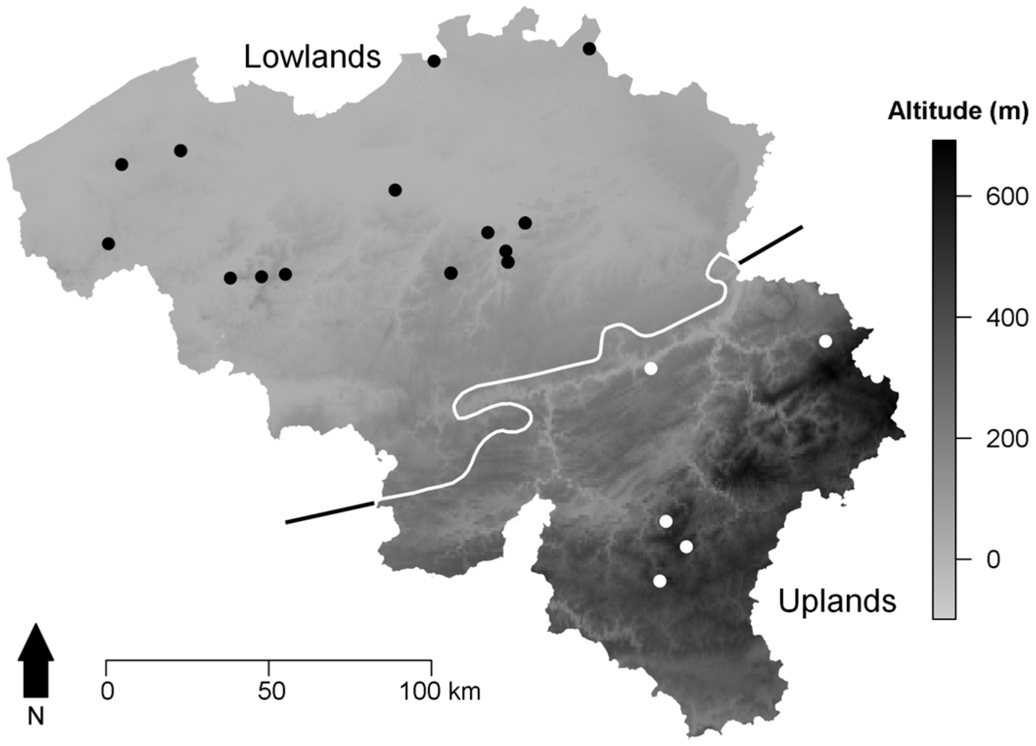
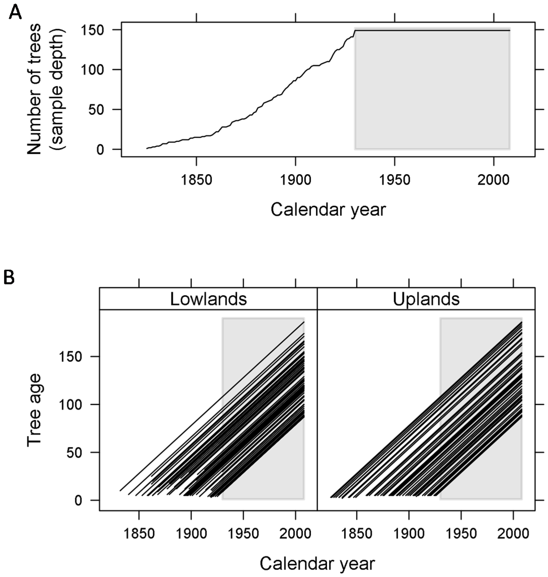
2.1. Tree Selection and Ring-Width Series

The dataset consisted of ring-width series of 149 beech trees selected across Belgium in fully stocked, regular and pure beech (>75% of stand basal area) high forests. Data were gathered from previous tree-growth modeling and dendroecological studies [25,26,32,33,44] (Table S1).

The dataset covered the two ecoregions of Belgium [45] (Figure 1): (1) the lowlands (84 trees) located in the North of the country in the maritime climate zone (mean altitude: 67 m; annual precipitation: 860 mm; annual mean temperature: 10.2 °C) and; (2) the uplands (65 trees) in the South, with hilly topography, in the sub-continental climate zone (mean altitude: 454 m; annual precipitation: 1140 mm; annual mean temperature: 8.1 °C). In the uplands, acid brown soils of 40–60 cm depth are mainly composed of loam with a high stone content. In the lowlands, deeper soils (>1 m) are composed of loam and/or sand in different proportions (Table S1).

In order to ensure maximum continuity in forest management, beech trees were selected from state forests. The selection of trees also ensured a good balance of tree-age range (87–186 years old) between the two ecoregions (Figure 2). All selected trees were dominant or co-dominant in order to limit the influence of inter-tree competition. Dominant trees face lower competition intensity and belong to a more stable population over time [15]. As beech is a shade-tolerant species, individual shifts in tree social status may occur among dominant populations but are less frequent in mature stands than in younger stands. This is especially the case in the context of Belgian hardwood state forests which are regularly thinned in favor of dominant trees. Furthermore, past changes in silvicultural practices in Belgium were less pronounced in mature stands. We ensured that the selected forests and trees, and the resulting ring-width series met the requirements of being representative of beech growth at the scale of the study region [25,32,46].

Two cores [25,26], two bars [32,33] or one disk [44] were extracted at breast height by tree. The tree-rings of each wood sample were measured to the nearest 1/100 mm from pith to bark, and averaged by tree. We ensured that tree series were correctly cross-dated by progressively detecting pointer years from the forest level to the whole country of Belgium level.

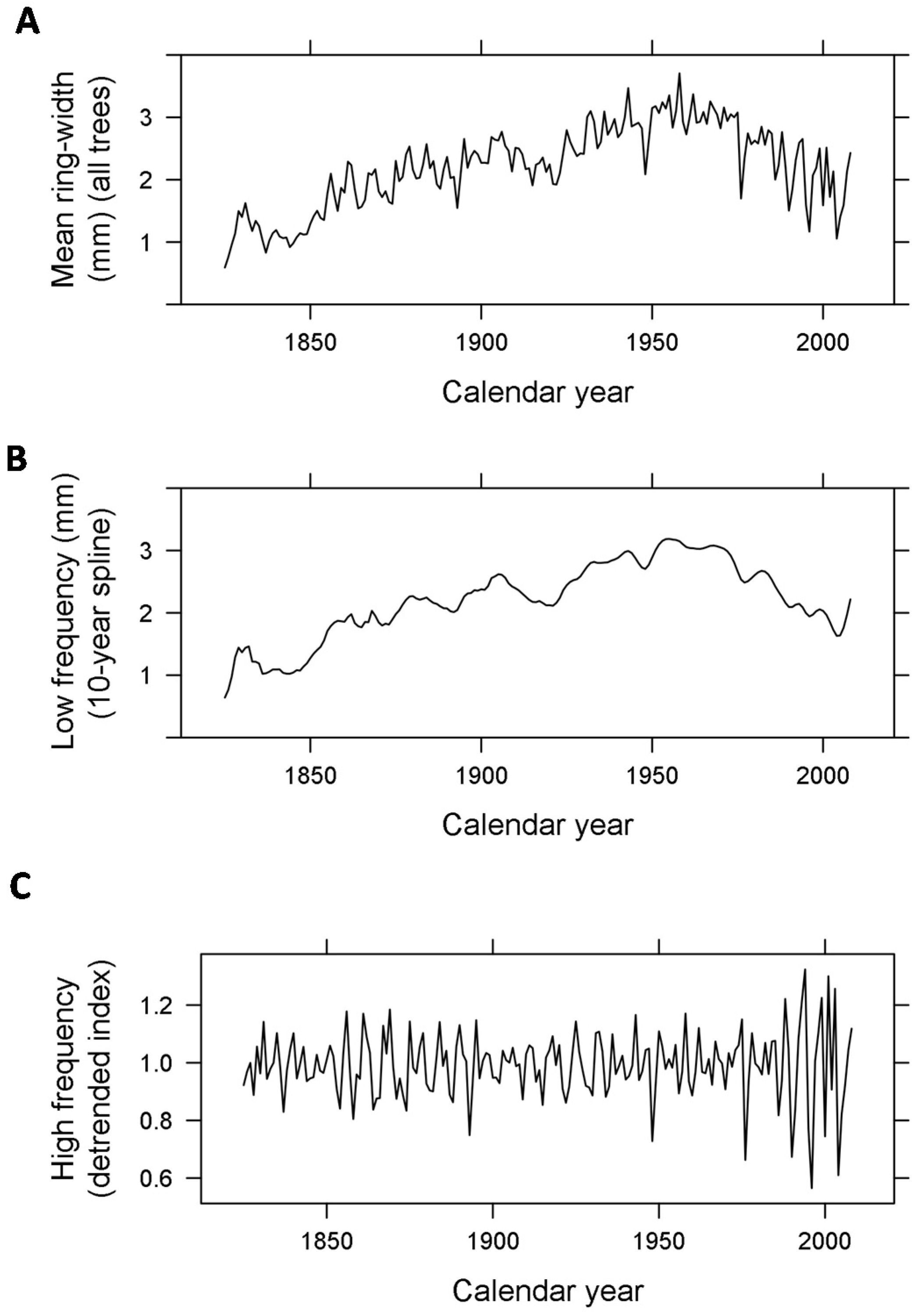
2.2. Low-Frequency Signal and High-Frequency Variability of Beech Ring-Width

The ring-width series of each tree was divided into a low- and a high-frequency signal (Figure 3) using the “dplR” package [47] implemented in the R software [48]. A flexible cubic smoothing spline (50% frequency cut-off at 10 years) was fitted to the ring-width series in order to extract the ring-width low frequency ($RWLF$). Although $RWLF$ included the medium-frequency signal as well (mainly influenced by thinning), the latter was not captured by the modeling procedure.

The high-frequency signal was computed as the ratio of ring-widths to the 10-year spline. This method of standardization results in a detrended index that maximizes the year-to-year variability, which is mostly related to climate [15]. The potential effects of the developmental stage on the high-frequency signal were maintained.

The high-frequency variability ($HFV$) was then estimated using generalized autoregressive conditional heteroscedasticity (GARCH) models by using the “fGarch” package [49] implemented in the R software [48]. $HFV$ was computed from the high-frequency signal of each tree as the conditional standard deviation of the fitted GARCH (1, 1) model. $HFV$ represents a better statistic to describe the variations in tree growth, compared to the mean sensitivity which has been reported previously as confusing and ambiguous [50].

2.3. Statistical Methodology, Model Formulation and Evaluation

The sampling design consisted of longitudinal data ($RLFW$ and $HFV$), which was structured according to three nested levels: ecoregion, forest, and tree. Such hierarchical structure allows the formulation parameters of mixed models to be tested and their variability at three different levels [51] to be estimated.

Model formulation (Equation (1)) was based on the studies of Bontemps et al. [23] and Aertsen et al. [26]. The non-linear models were fitted in two steps. Firstly, “size” models—$r\times f_1\left(rad\right)$—were fitted to estimate $RLFW$ and $HFV$ as a function of the tree radius using the Wykoff’s equation [52] (Equation (2)). $RLFW$ strongly increased up to a maximum before slowly decreasing; the $HFV$ pattern varied inversely (Figure S1). Secondly, “size-time” models—$r\times f_1\left(rad\right)\times f_2\left(yr\right)$ (Equation (1))—were fitted to include time-dependent (calendar year) effects by progressively testing linear, quadratic, cubic and spline functions [23] (Equation (3)). Time-dependent effects were tested over a common time period for all trees (1930−2008) in order to avoid potential biases due to sample depth variations (Figure 2); $f_2\left(yr\right)$ (Equation (3)) was forced to be equal to 1 before the year 1930.

$$Y=r\times f_1\left(rad\right)\times f_2\left(yr\right)+\epsilon$$

(1)

$Y$ refers to $RWLF$ or $HFV$, $r$ denotes the maximum $RWLF$ or the minimum $HFV$ (vertical scale parameter), $f_1\left(rad\right)$ denotes the function describing the size-dependent $Y$ variability, $rad$ denotes the tree radius (cm), $f_2\left(yr\right)$ denotes the function describing the time-dependent $Y$ variability, $yr$ denotes the calendar year, and $\epsilon$ designates the error term.

$$f_1\left(rad\right)=\left[{\left(\frac{rad}{s1}\right)}^{s2}\times exp\left(s2\times \frac{\left(1-{\left(\frac{rad}{s1}\right)}^2\right)}{2}\right)\right]$$

(2)

$s1$ and $s2$ are the “size” parameters: $s1$ denotes the $rad$ at which $r$ is reached (horizontal scale parameter) and $s2$ denotes the shape parameter.

$$f_2\left(yr\right)=1+{\displaystyle \sum }_{d=1}^n\left(t_d\times yr\right)$$

(3)

$t_d$ are the “time” parameters. The function $f_2\left(yr\right)$ is linear if $n$ = 1, quadratic if $n$ = 2, cubic if $n$ = 3 or a cubic spline if $n$ = 4.

All models were fitted using the maximum likelihood estimation (ML) by using the “nlme” package [53] implemented in the R software [48]. The significance of fixed and random parameter effects was tested progressively at ecoregion, forest, and tree level. Model improvement was confirmed by performing a likelihood ratio test (0.01 level of significance for the p-value) and by comparing the Akaike Information Criterion (AIC) between models.

2.4. Distinction of Size- and Time-Dependent Effects

The size- and time-dependent $Y$ variability of the whole country of Belgium and of the two ecoregions were computed using Equations (4) and (5), respectively, with the parameter estimates of the best “size-time” models (Equation (1)).

$$Y_s=r\times f_1\left(rad\right)$$

(4)

$$Y_t=r\times f_2\left(yr\right)$$

(5)

3. Results

3.1. Modeling Steps and Model Selection

The main steps for fitting “size” and “size-time” models of ring-width low frequency ($RWLF$) and high-frequency variability ($HFV$) are synthesized in

Table 1. Synthesis of the modeling steps of the ring-width low frequency models ($RWLF$, top) and the high-frequency variability models ($HFV$, bottom).

Ring-Width Low Frequency (RWLF) Models
Model	Parameters					AIC	p-value	rRMSE (%)	Mean Error (±Std. dev.)
	Fixed effects		Random effects
	Overall	Ecoregion	Ecoregion	Forest	Tree
size 1	$r$, s$1$, s$2$	/	/	/	/	51332	/	42.21	0.000 ± 1.052
size 2	$r$, s$1$, s$2$	/	$r$	/	/	51138	<0.001	41.97	0.000 ± 1.047
size 3	$r$, s$1$, s$2$	/	$r$	$r$	/	46253	<0.001	36.35	0.001 ± 0.906
size 4	$r$, s$1$, s$2$	/	$r$	$r$	$r$	42327	<0.001	31.91	0.001 ± 0.796
size-time 1	$r$, s$1$, s$2$, ${\mathrm{t}}_1$	/	$r$	$r$	$r$	41699	<0.001	31.36	0.003 ± 0.782
size-time 2	$r$ s$1$, s$2$, ${\mathrm{t}}_{1-2}$	/	$r$	$r$	$r$	41594	<0.001	31.26	0.002 ± 0.779
size-time 3	$r$, s$1$, s$2$, ${\mathrm{t}}_{1-3}$	/	$r$	$r$	$r$	41478	<0.001	31.16	0.002 ± 0.777
size-time 4	$r$, s$1$, s$2$, ${\mathrm{t}}_{1-4}$	/	$r$	$r$	$r$	41392	<0.001	31.08	0.002 ± 0.775
size-time 5	$r$, s$1$, s$2$, ${\mathrm{t}}_{1-4}$	${\mathrm{t}}_{1-4}$	$r$	$r$	$r$	41194	<0.001	30.90	0.002 ± 0.770
High-Frequency Variability (HFV) Models
Model	Parameters					AIC	p-value	rRMSE (%)	Mean Error (±Std. dev.)
	Fixed effects		Random effects
	Overall	Ecoregion	Ecoregion	Forest	Tree
size 1	$r$, s$1$, s$2$	/	/	/	/	−38724	/	3.20	0.000 ± 0.080
size 2	$r$, s$1$, s$2$	/	$r$	/	/	−39149	<0.001	3.16	0.000 ± 0.079
size 3	$r$, s$1$, s$2$	/	$r$	$r$	/	−41582	<0.001	2.94	0.000 ± 0.073
size 4	$r$, s$1$, s$2$	/	$r$	$r$	$r$	−43740	<0.001	2.72	0.000 ± 0.068
size-time 1	$r$, s$1$, s$2$, ${\mathrm{t}}_1$	/	$r$	$r$	$r$	−44305	<0.001	2.68	0.000 ± 0.067
size-time 2	$r$ s$1$, s$2$, ${\mathrm{t}}_{1-2}$	/	$r$	$r$	$r$	−44946	<0.001	2.63	0.000 ± 0.065
size-time 3	$r$, s$1$, s$2$, ${\mathrm{t}}_{1-3}$	/	$r$	$r$	$r$	−45299	<0.001	2.60	0.000 ± 0.065
size-time 4	$r$, s$1$, s$2$, ${\mathrm{t}}_{1-4}$	/	$r$	$r$	$r$	−45436	<0.001	2.59	0.000 ± 0.065
size-time 5	$r$, s$1$, s$2$, ${\mathrm{t}}_{1-4}$	${\mathrm{t}}_{1-4}$	$r$	$r$	$r$	−45663	<0.001	2.57	0.000 ± 0.064

Model parameters are defined in the Equations (1)–(3). rRMSE: relative root mean square error.

; the parameter estimates of the best“size 4” and “size-time 5” models are presented in

Table 2. Parameter estimates of the “size 4” models (top) and “size-time 5” models (bottom) for ring-width low frequency ($RWLF$, left) and for high-frequency variability ($HFV$, right).

“Size 4” Models
DF = 17400	$RWLF$			$HFV$
Fixed effects	Estimate	Standard error	p-value	Estimate	Standard error	p-value
$r$	3.14	0.144	<0.001	0.19	0.00712	<0.001
$s2$	0.304	0.0063	<0.001	−0.121	0.0038	<0.001
$s1$	15.1	0.1	<0.001	10.8	0.119	<0.001
Random effects	Ecoregion	Forest	Tree	Ecoregion	Forest	Tree
Std. dev. of $\mathrm{r}$	0.00528	0.664	0.582	0.00025	0.0295	0.0274
“Size-Time 5” Models
DF = 17300	$RWLF$			$\text{HFV}$
Fixed effects	Estimate	Standard error	p-value	Estimate	Standard error	p-value
$r$	3.36	0.256	<0.001	0.192	27.4	<0.001
$s2$	0.305	0.00662	<0.001	−0.0975	−21.7	<0.001
$s1$	19.7	0.476	<0.001	17.2	19.9	<0.001
$t_1$.(Intercept)	−0.753	0.136	<0.001	−0.115	−5.44	<0.001
$t_1$.Uplands	−0.641	0.22	0.00364	0.356	11.7	<0.001
$t_2$.(Intercept)	0.476	0.0561	<0.001	−0.0904	−4.29	<0.001
$t_2$.Uplands	0.193	0.0908	0.0334	0.0583	2.22	0.0264
$t_3$.(Intercept)	−0.332	0.0225	<0.001	0.509	7.88	<0.001
$t_3$.Uplands	0.157	0.0289	<0.001	−0.589	−6.61	<0.001
$t_4$.(Intercept)	−0.442	0.0172	<0.001	0.55	10.3	<0.001
$t_4.$Uplands	0.129	0.0204	<0.001	0.332	5.04	<0.001
Random effects	Ecoregion	Forest	Tree	Ecoregion	Forest	Tree
Std. dev. of $r$	0.263	0.708	0.542	0.0000191	0.0284	0.0263

Model parameters are defined in Equations (1)−(3). DF: degree of freedom.

. For each parameterized model, the distribution of residuals was graphically analyzed in relation to input variables to ensure they were unbiased and performed well. The improvement between the “size 4” and “size-time 5” models was significant. The inclusion of time-dependent effects significantly improved the goodness of fit (Table 1) and the distribution of residuals over time (Figure 4). Between 1930 and 2008, $f_2\left(yr\right)$ (Equation (3)) was in average equal to 0.96 (0.69–1.07) for $RWLF$, and 1.09 (0.98–1.60) for $HFV$. Additional plots of residuals and fitted values, illustrating the fitting quality of the models, are available in the supplementary material (Figures S2–S4).

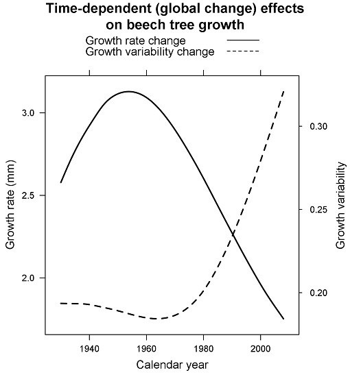
3.2. Size- and Time-Dependent Changes over Time

Size- and time-dependent changes in ring-width low frequency ($RWL{F}_s$ and $RWL{F}_t$, respectively) and high-frequency variability ($HF{V}_s$ and $HF{V}_t$, respectively) are shown in Figure 5. Both types of changes were estimated between 1930 and 2008 by using Equations (4) and (5), with the parameter estimates of the “size-time 5” models. $RWL{F}_t$ decreased by about 38% since the 1950–1960s, and $HF{V}_t$ increased by about 45% since the 1970–1980s. Both time-dependent changes (Figure 5) were highly similar to the size-time-dependent changes (i.e., combining both dependencies). Indeed, the change in $RWL{F}_s$ was limited to around 8%, and the change in $HF{V}_s$ was negligible.

The modeling procedure was necessary in order to eliminate the size-dependent effects over time. However, as these effects were mild, a visual analysis of raw data (i.e., ring-width series) would have been enough to highlight major changes in beech growth rate and growth variability (Figure 6). Time-dependent changes were more pronounced in the lowlands than in the uplands (Figure 7).

4. Discussion

We highlighted major time-dependent and size-independent changes over time in beech radial growth at the scale of Belgium. The effects of tree developmental stage (i.e., increasing tree size) were filtered out as they were related to a decline in forest productivity and to an increased sensitivity to disturbances [16,17,19,20]. Consequently, the highlighted changes cannot be attributed to size- or age-related processes. We identified changes in the low-frequency signal (growth rate) and in the high-frequency variability (growth variability), as they were related to different sources of change over time in the forest ecosystem.

The change in beech growth rate, that is an increase from the year 1930 (about +8%) and then a decrease from the 1950–1960s onwards (about −38%), confirms the results of previous studies on tree-growth modeling of beech in Northern Belgium (≈the lowlands) [25,26]. Nitrogen depositions have been related to increased carbon sequestration and productivity in European forests [54,55]. However, high nitrogen supply can lead to soil acidification and nutrient imbalances that would eventually alter tree physiology [56,57]. The decrease of beech growth was thus linked to an excess of soil nitrogen in Northern Belgium [25,26], where deposition levels prove to be among the highest in Europe [58]. The critical load of nutrient nitrogen is largely exceeded in Western Europe and Central Europe [59]. The main sources of nitrogen emissions are agriculture (mainly ammonia) and road transport (mainly nitrogen oxides).

Thinning practices mainly influenced the medium-frequency signal (i.e., growth fluctuations over several years to a decade) and were not taken into account in the modeling procedure. However, historical documents mention that Belgian forest managers have progressively increased thinning intensity since the middle of the 20th century, after a long tradition of high-density beech stands. Yet, it is unlikely that the decrease of beech growth rate is related to thinning practices. Indeed, higher thinning intensity is rather known to increase the growth rate and the resilience to climate of mature beech trees [60,61,62]. The widespread use of harvesting machines in Belgium is more likely responsible for the alteration of the soil ecology, with adverse consequences on tree growth [9]. Nowadays, adequate wood harvesting operations (e.g., limitation of machine activity on logging trails and use of mats of branches in coniferous stands) can help minimize soil compaction in managed forests. However, between the 1960s and 1990s, such operations were not regulated and thus were generally not implemented in Belgium. A considerable forest area may have been impacted by unrestricted traffic of harvesting machines during this period.

The increase of high-frequency growth variability from the 1970–1980s (about +45%) confirms the previous studies carried out in Southern Belgium (≈the uplands) [32,33]. Climate change has occurred quite homogeneously all over Belgium since the beginning of the 19th century. Between 1930 and 2008, temperatures have increased abruptly by about 1 °C at the end of the 1980s [39,40]. In the last decades, the increasing frequency and intensity of heat waves and related droughts have induced numerous and unusual reductions of beech yearly growth, and have led to remarkable synchronizations of beech tree growth at the regional scale [32].

To sum up, our results indicate that beech growth was negatively affected by two major factors: climate change and soil alteration (i.e., soil compaction and/or nitrogen deposition). Changes in beech growth rate and growth variability started in the 1950–60s and in the 1970–80s, respectively. Such 10- to 30-year difference indicates that the first half of the growth rate decrease was probably induced by soil alteration rather than by climate change. It remains difficult to evaluate the influence of nitrogen deposition on tree growth over time. The nitrogen cycle in forests is a complex process controlled by various biotic and abiotic factors, and nitrogen supply has been reported as positive at low levels and negative at elevated levels [54,57,58]. Nitrogen deposition evolves in a progressive manner with low yearly variations, and therefore could not be the main cause of increased beech growth variability. Furthermore, as compacted soils become more resistant to further compaction [9], the beech growth rate should have more or less stabilized a few decades after the 1960s. Therefore, the second half of the growth rate decrease is more probably related to climate change. Examination of beech radial growth at a yearly basis confirmed that frequent and intense growth reductions go along with a decreasing growth trend. The exceptionally hot and dry growing season of 1976 [29,63] could be considered as a transitional year (Figure 6).

Changes over time in beech growth rate and variability in the two ecoregions of Belgium were similar but more pronounced in the lowlands than in the uplands. Precipitation is higher in the uplands whereas soil water content and fertility are higher in the lowlands. Before the 1970s, the growth rate of beech trees was lower and their growth variability was higher in the uplands compared to the lowlands. These results are in accordance with previous dendroecological studies on beech. The sensitivity of beech to climate increases, while its radial growth decreases, with reduced soil water capacity [38]. In the case of a drought, higher soil water content can buffer drought stress more efficiently [64]. After the 1970s, the situation has tended to be the opposite. Beech forests in Belgium appear thus more vulnerable in the lowlands than in the uplands.

5. Conclusions

A declining tree growth can be an indicator of decreased vitality and of an increased risk of mortality [65]. Dying trees usually have lower growth rates, higher growth variability and an increased response to climate [66]. As the dieback and mortality of individual beech trees is still scarce and scattered in Belgium, we assume that beech has coped with global change up to now, but the question is: for how long? In the future, nitrogen emissions and depositions will likely keep decreasing [67]. However, the upcoming climate change, projected by the IPCC [68], will continue to weaken tree vitality [1,2]. Severe and recurrent droughts have been identified as a major factor contributing to accelerated rates of tree decline and mortality in Europe [3]. The agreement of the results from dendro-ecological, ecophysiological, and tree-growth modeling studies on beech across Europe is meaningful. Beech is impacted over a large part of its natural distribution. Forests in the South of the natural distribution are often considered most at risk. However, other areas may also be just as vulnerable [69]. Forest policy and management planning should now start to take this into consideration. Since other broadleaved tree species seem less impacted by climate change [70], a possible strategy would be to diversify tree species in managed beech forests [71,72].

References

1. Allen, C.D.; Macalady, A.K.; Chenchouni, H.; Bachelet, D.; McDowell, N.; Vennetier, M.; Kitzberger, T.; Rigling, A.; Breshears, D.D.; Hogg, E.H.; et al. A global overview of drought and heat-induced tree mortality reveals emerging climate change risks for forests. For. Ecol. Manag. 2010, 259, 660–684. [Google Scholar] [CrossRef]
2. Martínez-Vilalta, J.; Lloret, F.; Breshears, D.D. Drought-induced forest decline: Causes, scope and implications. Biol. Lett. 2012, 8, 689–691. [Google Scholar] [CrossRef] [PubMed]
3. Bréda, N.; Huc, R.; Granier, A.; Dreyer, E. Temperate forest trees and stands under severe drought: A review of ecophysiological responses, adaptation processes and long-term consequences. Ann. For. Sci. 2006, 63, 625–644. [Google Scholar] [CrossRef]
4. Waldner, P.; Marchetto, A.; Thimonier, A.; Schmitt, M.; Rogora, M.; Granke, O.; Mues, V.; Hansen, K.; Pihl Karlsson, G.; Žlindra, D.; et al. Detection of temporal trends in atmospheric deposition of inorganic nitrogen and sulphate to forests in Europe. Atmos. Environ. 2014, 95, 363–374. [Google Scholar] [CrossRef] [Green Version]
5. Guillemot, J.; Delpierre, N.; Vallet, P.; François, C.; Martin-StPaul, N.K.; Soudani, K.; Nicolas, M.; Badeau, V.; Dufrêne, E. Assessing the effects of management on forest growth across France: Insights from a new functional–structural model. Ann. Bot. 2014, 114, 779–793. [Google Scholar] [CrossRef] [PubMed]
6. Trouvé, R.; Bontemps, J.D.; Collet, C.; Seynave, I.; Lebourgeois, F. Growth partitioning in forest stands is affected by stand density and summer drought in sessile Oak and Douglas-fir. For. Ecol. Manag. 2014, 334, 358–368. [Google Scholar] [CrossRef]
7. D’Amato, A.W.; Bradford, J.B.; Fraver, S.; Palik, B.J. Effects of thinning on drought vulnerability and climate response in north temperate forest ecosystems. Ecol. Appl. 2013, 23, 1735–1742. [Google Scholar] [CrossRef] [PubMed]
8. Lebourgeois, F.; Eberlé, P.; Mérian, P.; Seynave, I. Social status-mediated tree-ring responses to climate of Abies alba and Fagus sylvatica shift in importance with increasing stand basal area. For. Ecol. Manag. 2014, 328, 209–218. [Google Scholar] [CrossRef]
9. Cambi, M.; Certini, G.; Neri, F.; Marchi, E. The impact of heavy traffic on forest soils: A review. For. Ecol. Manag. 2015, 338, 124–138. [Google Scholar] [CrossRef]
10. Speer, J.H. Fundamentals of Tree-Ring Research; University of Arizona Press: Tucson, AZ, USA, 2010; p. 368. [Google Scholar]
11. Fritts, H.C. Tree Rings and Climate; Academic Press: London, UK, 1976; p. 567. [Google Scholar]
12. Fritts, H.C.; Swetnam, T.W. Dendroecology: A tool for evaluating variations in past and present forest environments. Adv. Ecol. Res. 1989, 19, 111–188. [Google Scholar]
13. Weiskittel, A.R.; Hann, D.W.; Kershaw, J.A.; Vanclay, J.K. Forest Growth and Yield Modeling; Wiley-Blackwell: Hoboken, NJ, USA, 2011; p. 430. [Google Scholar]
14. Bowman, D.M.J.S.; Brienen, R.J.W.; Gloor, E.; Phillips, O.L.; Prior, L.D. Detecting trends in tree growth: Not so simple. Trends Plant Sci. 2013, 18, 11–17. [Google Scholar] [CrossRef] [PubMed]
15. Cook, E.R.; Kairiukstis, L.A. Methods of dendrochronology: Applications in the environmental sciences; Kluwer Academic Publishers: Boston, MA, USA, 1990; p. 394. [Google Scholar]
16. Rozas, V.; DeSoto, L.; Olano, J.M. Sex-specific, age-dependent sensitivity of tree-ring growth to climate in the dioecious tree Juniperus thurifera. New Phytol. 2009, 182, 687–697. [Google Scholar] [CrossRef] [PubMed]
17. Genet, H.; Bréda, N.; Dufrêne, E. Age-related variation in carbon allocation at tree and stand scales in beech (Fagus sylvatica L.) and sessile oak (Quercus petraea (Matt.) Liebl.) using a chronosequence approach. Tree Physiol. 2009, 30, 177–192. [Google Scholar] [CrossRef] [PubMed]
18. Copenheaver, C.A.; Crawford, C.J.; Fearer, T.M. Age-specific responses to climate identified in the growth of Quercus alba. Trees-Struct. Funct. 2011, 25, 647–653. [Google Scholar] [CrossRef]
19. Mérian, P.; Lebourgeois, F. Size-mediated climate-growth relationships in temperate forests: A multi-species analysis. For. Ecol. Manag. 2011, 261, 1382–1391. [Google Scholar] [CrossRef]
20. Rozas, V. Individual-based approach as a useful tool to disentangle the relative importance of tree age, size and inter-tree competition in dendroclimatic studies. For. Biogeosci. For. 2015, 8, 187–194. [Google Scholar] [CrossRef]
21. Mencuccini, M.; Martínez-Vilalta, J.; Vanderklein, D.; Hamid, H.A.; Korakaki, E.; Lee, S.; Michiels, B. Size-mediated ageing reduces vigour in trees. Ecol. Lett. 2005, 8, 1183–1190. [Google Scholar] [CrossRef] [PubMed]
22. Geßler, A.; Keitel, C.; Kreuzwieser, J.; Matyssek, R.; Seiler, W.; Rennenberg, H. Potential risks for European beech (Fagus sylvatica L.) in a changing climate. Trees-Struct. Funct. 2007, 21, 1–11. [Google Scholar] [CrossRef]
23. Bontemps, J.D.; Hervé, J.C.; Dhôte, J.F. Dominant radial and height growth reveal comparable historical variations for common beech in north-eastern France. For. Ecol. Manag. 2010, 259, 1455–1463. [Google Scholar] [CrossRef]
24. Charru, M.; Seynave, I.; Morneau, F.; Bontemps, J.D. Recent changes in forest productivity: An analysis of national forest inventory data for common beech (Fagus sylvatica L.) in north-eastern France. For. Ecol. Manag. 2010, 260, 864–874. [Google Scholar] [CrossRef]
25. Kint, V.; Aertsen, W.; Campioli, M.; Vansteenkiste, D.; Delcloo, A.; Muys, B. Radial growth change of temperate tree species in response to altered regional climate and air quality in the period 1901–2008. Clim. Chang. 2012, 115, 343–363. [Google Scholar] [CrossRef]
26. Aertsen, W.; Janssen, E.; Kint, V.; Bontemps, J.D.; van Orshoven, J.; Muys, B. Long-term growth changes of common beech (Fagus sylvatica L.) are less pronounced on highly productive sites. For. Ecol. Manag. 2014, 312, 252–259. [Google Scholar] [CrossRef]
27. Dittmar, C.; Zech, W.; Elling, W. Growth variations of common beech (Fagus sylvatica L.) under different climatic and environmental conditions in Europe—A dendroecological study. For. Ecol. Manag. 2003, 173, 63–78. [Google Scholar] [CrossRef]
28. Friedrichs, D.A.; Trouet, V.; Büntgen, U.; Frank, D.C.; Esper, J.; Neuwirth, B.; Löffler, J. Species-specific climate sensitivity of tree growth in Central-West Germany. Trees-Struct. Funct. 2009, 23, 729–739. [Google Scholar] [CrossRef]
29. Scharnweber, T.; Manthey, M.; Criegee, C.; Bauwe, A.; Schröder, C.; Wilmking, M. Drought matters—Declining precipitation influences growth of Fagus sylvatica L. and Quercus robur L. in north-eastern Germany. For. Ecol. Manag. 2011, 262, 947–961. [Google Scholar] [CrossRef]
30. Weber, P.; Bugmann, H.; Pluess, A.R.; Walthert, L.; Rigling, A. Drought response and changing mean sensitivity of European beech close to the dry distribution limit. Trees-Struct. Funct. 2013, 27, 171–181. [Google Scholar] [CrossRef]
31. Castagneri, D.; Nola, P.; Motta, R.; Carrer, M. Summer climate variability over the last 250 years differently affected tree species radial growth in a mesic Fagus-Abies-Picea old-growth forest. For. Ecol. Manag. 2014, 320, 21–29. [Google Scholar] [CrossRef]
32. Latte, N.; Lebourgeois, F.; Claessens, H. Increased tree-growth synchronization of beech (Fagus sylvatica L.) in response to climate change in northwestern Europe. Dendrochronologia 2015, 33, 69–77. [Google Scholar] [CrossRef]
33. Latte, N.; Kint, V.; Drouet, T.; Penninckx, V.; Lebourgeois, F.; Vanwijnsberghe, S.; Claessens, H. Dendroécologie du Hêtre en Forêt de Soignes. Les cernes des arbres nous renseignent sur les changements récents et futurs. Forêt Nat. 2015, 137, 24–37. [Google Scholar]
34. Jump, A.S.; Hunt, J.M.; Pen̈uelas, J. Rapid climate change-related growth decline at the southern range edge of Fagus sylvatica. Glob. Chang. Biol. 2006, 12, 2163–2174. [Google Scholar] [CrossRef]
35. Piovesan, G.; Biondi, F.; Di Filippo, A.; Alessandrini, A.; Maugeri, M. Drought-driven growth reduction in old beech (Fagus sylvatica L.) forests of the central Apennines, Italy. Glob. Chang. Biol. 2008, 14, 1265–1281. [Google Scholar] [CrossRef]
36. Di Filippo, A.; Biondi, F.; Maugeri, M.; Schirone, B.; Piovesan, G. Bioclimate and growth history affect beech lifespan in the Italian Alps and Apennines. Glob. Chang. Biol. 2012, 18, 960–972. [Google Scholar] [CrossRef]
37. Bolte, A.; Hilbrig, L.; Grundmann, B.; Kampf, F.; Brunet, J.; Roloff, A. Climate change impacts on stand structure and competitive interactions in a southern Swedish spruce-beech forest. Eur. J. For. Res. 2010, 129, 261–276. [Google Scholar] [CrossRef]
38. Lebourgeois, F.; Bréda, N.; Ulrich, E.; Granier, A. Climate-tree-growth relationships of European beech (Fagus sylvatica L.) in the French Permanent Plot Network (RENECOFOR). Trees-Struct. Funct. 2005, 19, 385–401. [Google Scholar] [CrossRef]
39. Demarée, G.R.; Lachaert, P.J.; Verhoeve, T.; Thoen, E. The long-term daily central Belgium temperature (CBT) series (1767–1998) and early instrumental meteorological observations in Belgium. Clim. Chang. 2002, 53, 269–293. [Google Scholar] [CrossRef]
40. IRM. Vigilance Climatique. Institut Royal Météorologique de Belgique, 2015. Available online: http://www.meteo.be/resources/20150508vigilance-oogklimaat/vigilance_climatique_IRM_2015_WEB_FR_BAT.pdf (accessed on 15 April 2016).
41. Dobbertin, M. Tree growth as indicator of tree vitality and of tree reaction to environmental stress: A review. Eur. J. For. Res. 2005, 124, 319–333. [Google Scholar] [CrossRef]
42. Greenwood, D.L.; Weisberg, P.J. Density-dependent tree mortality in pinyon-juniper woodlands. For. Ecol. Manag. 2008, 255, 2129–2137. [Google Scholar] [CrossRef]
43. Linares, J.C.; Camarero, J.J. From pattern to process: Linking intrinsic water-use efficiency to drought-induced forest decline. Glob. Chang. Biol. 2012, 18, 1000–1015. [Google Scholar] [CrossRef]
44. Latte, N.; Lebourgeois, F.; Claessens, H. Growth partitioning within beech trees (Fagus sylvatica L.) varies in response to summer heat waves and related droughts. Trees-Struct. Funct. 2016, 30, 189–201. [Google Scholar] [CrossRef] [Green Version]
45. Campioli, M.; Vincke, C.; Jonard, M.; Kint, V.; Demarée, G.; Ponette, Q. Current status and predicted impact of climate change on forest production and biogeochemistry in the temperate oceanic European zone: Review and prospects for Belgium as a case study. J. For. Res. 2012, 17, 1–18. [Google Scholar] [CrossRef]
46. Mérian, P.; Bert, D.; Lebourgeois, F. An approach for quantifying and correcting sample size-related bias in population estimates of climate-tree growth relationships. For. Sci. 2013, 59, 444–452. [Google Scholar] [CrossRef]
47. Bunn, A.G. A dendrochronology program library in R (dplR). Dendrochronologia 2008, 26, 115–124. [Google Scholar] [CrossRef]
48. The R Core Team. R: A language and Environment for Statistical Computing. Available online: http://r-project.org/ (accessed on 5 August 2016).
49. Wuertz, D.; Chalabi, Y.; Miklovic, M.; Boudt, C.; Chausse, P. fGarch: Rmetrics—Autoregressive Conditional Heteroskedastic Modelling. Available online: http://CRAN.R-project.org/package=fGarch (accessed on 5 August 2016).
50. Bunn, A.G.; Jansma, E.; Korpela, M.; Westfall, R.D.; Baldwin, J. Using simulations and data to evaluate mean sensitivity (ζ) as a useful statistic in dendrochronology. Dendrochronologia 2013, 31, 250–254. [Google Scholar] [CrossRef]
51. Pinheiro, J.; Bates, D. Mixed Effects Models in S and S-PLUS; SpringerVerlag: New York, NY, USA, 2000; p. 528. [Google Scholar]
52. Wykoff, W.R. A basal area increment model for individual conifers in the northern Rocky Mountains. For. Sci. 1990, 36, 1077–1104. [Google Scholar]
53. Pinheiro, J.; Bates, D.; DebRoy, S.; Sarkar, D.; R Core Team. nlme: Linear and Nonlinear Mixed Effects Models. Available online: http://CRAN.R-project.org/package=nlme (accessed on 5 August 2016).
54. Magnani, F.; Mencuccini, M.; Borghetti, M.; Berbigier, P.; Berninger, F.; Delzon, S.; Grelle, A.; Hari, P.; Jarvis, P.G.; Kolari, P.; et al. The human footprint in the carbon cycle of temperate and boreal forests. Nature 2007, 447, 848–850. [Google Scholar] [CrossRef] [PubMed]
55. Bontemps, J.D.; Hervé, J.C.; Leban, J.M.; Dhôte, J.F. Nitrogen footprint in a long-term observation of forest growth over the twentieth century. Trees-Struct. Funct. 2011, 25, 237–251. [Google Scholar] [CrossRef]
56. Braun, S.; Thomas, V.F.D.; Quiring, R.; Flückiger, W. Does nitrogen deposition increase forest production? The role of phosphorus. Environ. Pollut. 2010, 158, 2043–2052. [Google Scholar] [CrossRef] [PubMed]
57. Zhu, X.; Zhang, W.; Chen, H.; Mo, J. Impacts of nitrogen deposition on soil nitrogen cycle in forest ecosystems: A review. Acta Ecol. Sin. 2015, 35, 35–43. [Google Scholar] [CrossRef]
58. De Vries, W.; Reinds, G.J.; Posch, M.; Sanz, M.J.; Krause, G.H.M.; Calatayud, V.; Renaud, J.P.; Dupouey, J.L.; Sterba, H.; Vel, E.M.; et al. Intensive Monitoring of Forest Ecosystems in Europe: Technical Report; UnEce: Brussels, Belgium, 2003. [Google Scholar]
59. European Environment Agency (EEA). Air Pollution in Europe 1990–2004: EEA Report No 2/2007; European Environment Agency: Copenhagen, Denmark, 2007. [Google Scholar]
60. Le Goff, N.; Ottorin, J.M. Effects of thinning on beech growth. Interaction with climatic factors. Rev. Forest. Fr. 1999, 51, 355–364. [Google Scholar]
61. Van der Maaten, E. Thinning prolongs growth duration of European beech (Fagus sylvatica L.) across a valley in southwestern Germany. For. Ecol. Manag. 2013, 306, 135–141. [Google Scholar] [CrossRef]
62. Diaconu, D.; Kahle, H.P.; Spiecker, H. Tree- and stand-level thinning effects on growth of European Beech (Fagus sylvatica L.) on a Northeast- and a Southwest-facing slope in Southwest Germany. Forests 2015, 6, 3256–3277. [Google Scholar] [CrossRef]
63. Penninckx, V.; Meerts, P.; Herbauts, J.; Gruber, W. Ring width and element concentrations in beech (Fagus sylvatica L.) from a periurban forest in central Belgium. For. Ecol. Manag. 1999, 113, 23–33. [Google Scholar] [CrossRef]
64. Lévesque, M.; Walthert, L.; Weber, P. Soil nutrients influence growth response of temperate tree species to drought. J. Ecol. 2016, 104, 377–387. [Google Scholar] [CrossRef]
65. Gillner, S.; Rüger, N.; Roloff, A.; Berger, U. Low relative growth rates predict future mortality of common beech (Fagus sylvatica L.). For. Ecol. Manag. 2013, 302, 372–378. [Google Scholar] [CrossRef]
66. Camarero, J.J.; Gazol, A.; Sangüesa-Barreda, G.; Oliva, J.; Vicente-Serrano, S.M. To die or not to die: Early warnings of tree dieback in response to a severe drought. J. Ecol. 2015, 103, 44–57. [Google Scholar] [CrossRef]
67. Engardt, M.; Langner, J. Simulations of future sulphur and nitrogen deposition over Europe using meteorological data from three regional climate projections. Available online: http://dx.doi.org/10.3402/tellusb.v65i0.20348 (accessed on 5 August 2016).
68. IPCC. Climate Change 2014: Synthesis Report. In Contribution of Working Groups I, II and III to the Fifth Assessment Report of the Intergovernmental Panel on Climate Change; IPPC: Geneva, Switzerland, 2014. [Google Scholar]
69. Hacket-Pain, A.J.; Cavin, L.; Friend, A.D.; Jump, A.S. Consistent limitation of growth by high temperature and low precipitation from range core to southern edge of European beech indicates widespread vulnerability to changing climate. Eur. J. For. Res. 2016, 1–13. [Google Scholar] [CrossRef]
70. Zimmermann, J.; Hauck, M.; Dulamsuren, C.; Leuschner, C. Climate warming-related growth decline affects Fagus sylvatica, but not other broad-leaved tree species in central European mixed forests. Ecosystems 2015, 18, 560–572. [Google Scholar] [CrossRef]
71. Lindner, M.; Maroschek, M.; Netherer, S.; Kremer, A.; Barbati, A.; Garcia-Gonzalo, J.; Seidl, R.; Delzon, S.; Corona, P.; Kolström, M.; et al. Climate change impacts, adaptive capacity, and vulnerability of European forest ecosystems. For. Ecol. Manag. 2010, 259, 698–709. [Google Scholar] [CrossRef]
72. Metz, J.; Annighöfer, P.; Schall, P.; Zimmermann, J.; Kahl, T.; Schulze, E.-D.; Ammer, C. Site-adapted admixed tree species reduce drought susceptibility of mature European beech. Glob. Chang. Biol. 2016, 22, 903–920. [Google Scholar] [CrossRef] [PubMed]
Figure 1. Locations of the selected beech forests in the lowlands (black dots) and in the uplands (white dots) in Belgium. Darker grey indicates higher elevation (m). The white line indicates the boundary between the two ecoregions (lowlands in the North and uplands in the South).
Forests 07 00174 g001
Figure 2. (A), number of trees over time (sample depth). (B), age over time of the 149 beech trees (84 in lowlands, 65 in uplands). The grey rectangles indicate the period 1930–2008, common to all the trees (i.e., with constant sample depth). Tree age was estimated as the number of rings from pith to bark plus 5 (i.e., the number of years to reach the breast height). In the case of cores with missing pith rings, the estimation of tree age was based on field information provided by forest managers.
Forests 07 00174 g002
Figure 3. From (A) to (C), mean ring-width, low-frequency signal and high-frequency signal of the 149 beech trees. The radial growth of each of the beech trees was similarly divided into a low- and a high-frequency signal.
Forests 07 00174 g003
Figure 4. Residuals (grey dots) over time of the “size 4” models (A,B) and “size-time 5” models (C,D) of ring-width low frequency ( R W L F , A,C) and high-frequency variability ( H F V , B,D). Darker areas indicate the period 1930–2008, common to all trees. Lines indicate mean trends (LOESS). The inclusion of the time-dependent effects improved greatly the distribution of residuals over time.
Forests 07 00174 g004
Figure 5. Long-term changes over time in ring-width low frequency ( R W L F , A, B) and high-frequency variability ( H F V , C, D). Size-time dependent effects (A, C; Equation (1)) were divided into size-dependent (B, D, dashed lines; Equation (4)) and time-dependent (B, D, full lines; Equation (5)) effects. Size-dependent changes are low in comparison to time-dependent changes.
Forests 07 00174 g005
Figure 6. Mean radial growth of the 149 beech trees with 10-year moving mean, minimum, and maximum trends to illustrate the increased yearly growth reductions and their influence on the overall growth decrease.
Forests 07 00174 g006
Figure 7. Long-term and time-dependent changes over time in ring-width low frequency (A) and high-frequency variability (B) for lowlands (full lines) and uplands (dashed lines). Both changes were more pronounced in lowlands than in uplands.
Forests 07 00174 g007