Tree Stem Diameter Estimation from Mobile Laser Scanning Using Line-Wise Intensity-Based Clustering

Abstract

Diameter at breast height has been estimated from mobile laser scanning using a new set of methods. A 2D laser scanner was mounted facing forward, tilted nine degrees downwards, on a car. The trajectory was recorded using inertial navigation and visual SLAM (simultaneous localization and mapping). The laser scanner data, the trajectory and the orientation were used to calculate a 3D point cloud. Clusters representing trees were extracted line-wise to reduce the effects of uncertainty in the positioning system. The intensity of the laser echoes was used to filter out unreliable echoes only grazing a stem. The movement was used to obtain measurements from a larger part of the stem, and multiple lines from different views were used for the circle fit. Two trigonometric methods and two circle fit methods were tested. The best results with bias 2.3% (6 mm) and root mean squared error 14% (37 mm) were acquired with the circle fit on multiple 2D projected clusters. The method was evaluated compared to field data at five test areas with approximately 300 caliper-measured trees within a 10-m working range. The results show that this method is viable for stem measurements from a moving vehicle, for example a forest harvester.

1. Introduction

The developing field of precision forestry requires detailed information about forest stands, such as diameter at breast height (DBH) and stem positions of the trees within the stands [1]. One convenient method to collect the information is to acquire data from a moving vehicle, such as a forest harvester, during thinning operations or from an inventory using an off-road vehicle. A sensor mounted on a forest harvester could record information about trees that were harvested, as well as those left in the forest. This information would give a valuable inventory after thinning to update the forest owner’s information about the forest stand and the estimations of wood volume and biomass. If the sensor data could be processed in real time, the gathered information could be used for decision support for the operator or for assisted/autonomous control of the machine. Another purpose of mobile collection of stem data would be for navigation assistance in forests [2,3]. The precision of satellite navigation is affected by multi-path effects induced by the forest canopy, which makes the positioning unreliable. For these reasons, research regarding algorithms that can deliver accurate DBH from mobile laser scanners is of interest.

Various methods for the estimation of DBH and tree positions using a stationary 3D terrestrial laser scanner (TLS) in single or multiple scan positions have been developed, beginning with [4,5,6]. Many methods have delivered promising results and can be used for plot inventory [7,8,9]. Trees are visible from multiple views by using multi-scan TLS, which can also give detailed tree positions at the stand level. An advantage of 3D scanning compared to traditional measurements is that stem profiles can be extracted [8,10]. When a stem profile is made, the above-ground biomass can be estimated [11,12,13,14]. However, as there are many calculations involved in the process of deriving forest parameters from TLS data, the results can be biased due to many reasons, such as the influence of the TLS scan mode on circle fitting [15] and the intensity incidence angle effect [16]. TLS applications collect a large amount of data, and the computational costs can also be high. Simplifications using low-resolution 3D data can be done, and algorithms using knowledge about the object-scanner geometry can be used to reduce the calculation load [17,18].

Mobile laser scanning (MLS) is of interest for navigation and mobile mapping. A simple 2D laser scanner mounted on a moving vehicle can produce a map of the traversed area, if the trajectory of the vehicle is recorded simultaneously. The point clouds generated by MLS are generally of lower quality than those generated from stationary TLS. One of the common problems is that the position of the scanner is hard to estimate with enough precision to co-register the point cloud successfully. In structured environments, with for example vertical and flat surfaces like walls, identified objects can be used to determine the position. However, in unstructured environments, such as forests, it is hard to predict the features in the environment, and such a positioning system is unreliable [19]. Another problem is the precision of the commonly-used mobile laser scanners. They are usually less expensive than their 3D counterparts, and they often have lower angular resolution and wider laser beams, giving larger footprints. These characteristics give sparser point clouds with higher errors in each point, especially on slanted surfaces, such as the flanks on a cylindrical object. Tree stems, of which diameter estimations are of interest in forestry applications, are affected by this phenomenon. This problem affects circle fit methods, which overestimate the diameters grossly, and trigonometric methods using the viewing angle and the distance to the tree that are preferred by Brunner and Gizachew [19], Ringdahl et al. [20] and Jutila et al. [21]. The wide range of results that are reported for estimations of DBH from MLS are complicated to compare due to different metrics and different methods for evaluation. Basal area has been derived by Brunner and Gizachew [19] with errors of around 10 m${}^2$/ha for individual scans. DBH with relative error of 4% has been reported by Jutila et al. [21]. The precision of various methods has been studied in a controlled environment without branches and occlusions by Ringdahl et al. [20]; with improvements of a trigonometric method, they have reduced the error of the best method to 12%. Circle fit with very small errors, 4.29 mm, has been achieved by Dian et al. [22], but their comparison materials are measurements in the point cloud without accounting for the physical error of the laser measurements. In a laboratory setting, the radius of tree trunks has been estimated with a relative bias of 4% by Kong et al. [23]; however, they used multiple stationary scans at the same height to reduce the influence of statistical errors in the distance measurement.

The position and the orientation of the scanner are crucial for the quality of an MLS point cloud. An angle error ${\epsilon }_v$ of the laser scanner direction propagates at distance D according to ${\epsilon }_D=\sin \left({\epsilon }_v\right)\times D$; for example, ${\epsilon }_v=1^o$ gives an error ${\epsilon }_d=17.5$ cm at $D=10$ m distance. A position error simply translates the points: a 1-cm position error of the laser scanner gives a 1-cm point error. Global Navigation Satellite Systems (GNSS) are commonly used for navigation and positioning purposes. Inexpensive equipment, such as smartphones, can have meter precision under good circumstances, but the precision depends on signal quality and the line of sight to the positioning satellites. In forests, the signals are attenuated by the canopy. This reduces the accuracy even further, and meter precision is not reached on the ground [24]. A combination of GNSS and INS (inertial navigation system)/IMU (inertial measurement unit) that uses accelerometers and gyroscopic sensors can support the GNSS to estimate a better position in difficult conditions [25]. However, there is a common problem with drift in INS, especially in less expensive and lighter systems. Visual information (or laser scanning/radar data) can be used for the estimation of positions using simultaneous localization and mapping (SLAM) [26]. SLAM is often used in combination with INS and can compensate for drift, but distinctive feature points are needed to calculate the position. In environments where distinctive feature points are hard to find, SLAM methods are problematic. An MLS system (the same as used in [21]) was positioned with SLAM using 2D laser data as input [2]. The system was usable in small loops (e.g., 50 m × 100 m), but the accumulated error from larger loops was unacceptably high. They also tested SLAM using synchronized cameras, but did not obtain usable results. Tree positions in triplets making triangles were used for the positioning, with the aim of the positioning of forestry machines. The errors in the point cloud were not stated. Centimeter precision using a smartphone quality GNSS antenna is achieved by [27]. Methods to reduce the computational load to reach centimeter precision with combined GPS/IMU in real time, even in challenging environments, is presented by [28]. In any case, centimeter precision is not enough for the co-registration of lines into a point cloud, if the cloud should be processed with common 3D TLS algorithms.

In this article, we follow-up an earlier project by SLU (Swedish University of Agricultural Sciences), Skogforsk (Forestry Research Institute of Sweden) and FOI (Swedish Defence Research Agency) [29], where a prototype system for mobile laser scanning of forests was constructed. A 2D laser scanner was mounted forward-facing on a car, and the trajectory was recorded using a combination of inertial navigation and visual SLAM. During a field campaign, data were collected from five forest stands for which partial field data were also collected. The laser scanner data were co-registered into a 3D point cloud using the trajectory data and the orientation of the scanner. DBH was estimated using slightly adapted methods for TLS point clouds [9] with an RMSE of 24% (5.8 cm) and a bias of −1.9% (−0.5 cm). The small bias indicates that the method is usable for the aggregation of results, such as the estimation of the basal area on the stand level. However, for single tree estimations, the method’s value is low, since the RMSE is large. The large RMSE is presumably caused by errors in the positioning, which made the point cloud noisy. We present methods to estimate the DBH of the trees using the special characteristics of this 2D/3D point cloud to line-wise extract features and then only use the 3D information for positioning of the stems.

2. Materials and Methods

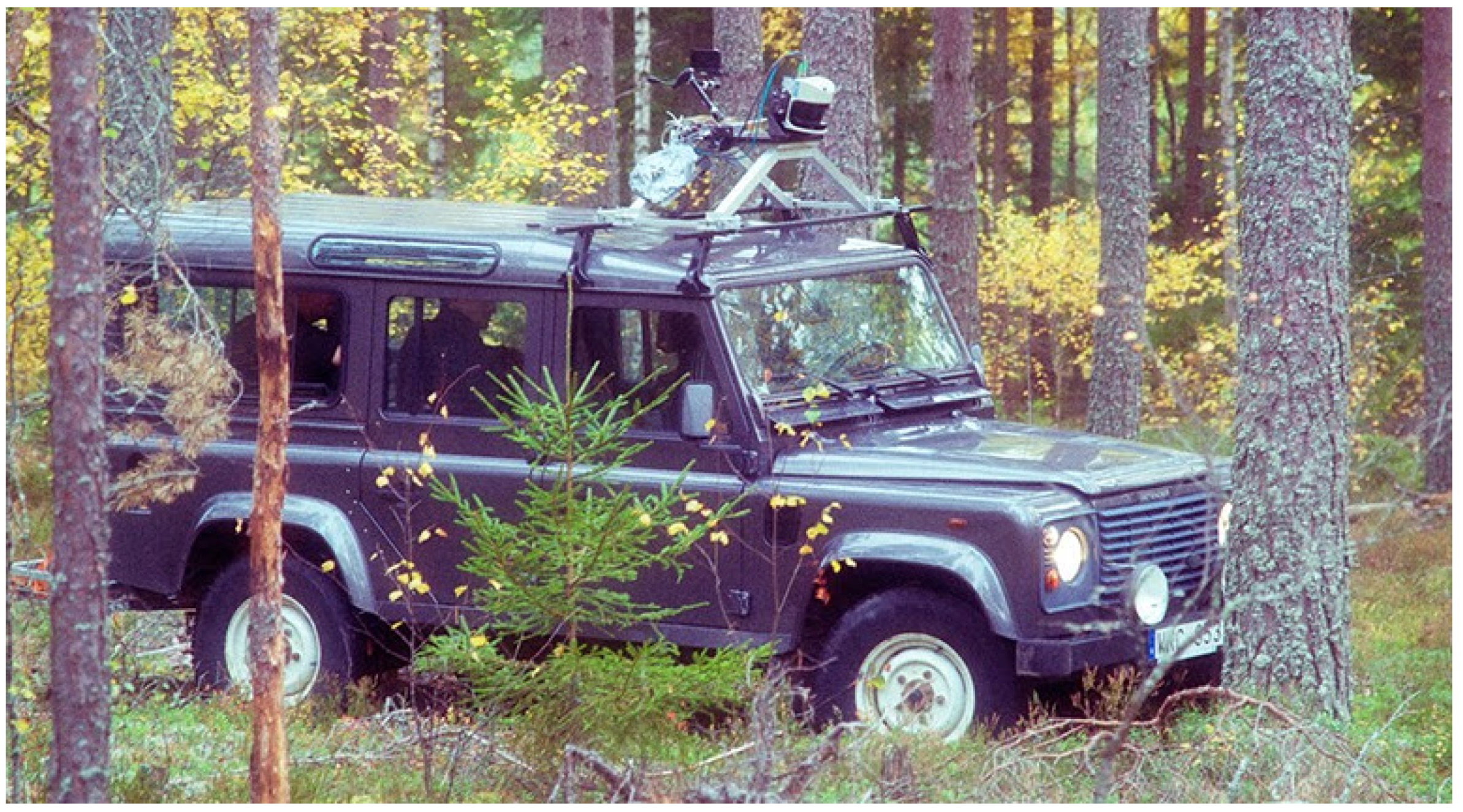
2.1. Data Collection

Data were collected at five different sites in Östergötland, Sweden, in November 2013. The locations included various forest types, with different terrain conditions. In

Table 1. Summary of the test sites.

Site	Stems/ha	DBH Mean (cm)	Height (m)	Species	Terrain Type
	Basal Area (m2/ha)	Range (cm)			Understory
Älvan	812	23	23	Spruce	Flat
	44	5–38		(Picea abies L.)	Low
Malmköping 1	366	24	26	Young pine	Flat
	17	5–39		(Pinus sylvestris L.)	Occasional
Malmköping 2	509	18	15	Young pine	Broken
	17	3–34		(Pinus sylvestris L.)	Occasional
Sonstorp 1	668	27	32	Spruce	Flat
	37	6–46		(Picea abies L.)	Occasional
Sonstorp 2	573	23	25	Spruce	Broken
	35	7–37		(Picea abies L.)	Occasional

, a summary of the locations is presented.

2.2. Reference Data

Reference data were collected at 20 × 20 m-wide field plots adjacent to the traversed track. DBH was collected using a caliper, and the trees were positioned using ultrasonic trilateration with POSTEX equipment [30]. Four reference trees on each plot were manually identified in the MLS point cloud and used for transformation of the field trees’ coordinates into the point cloud coordinates. The tree height data were extracted from the Swedish forest attribute map [31,32], based on airborne laser scanning and national forest inventory data. A summary of the reference data is presented in Table 1.

2.3. System Description

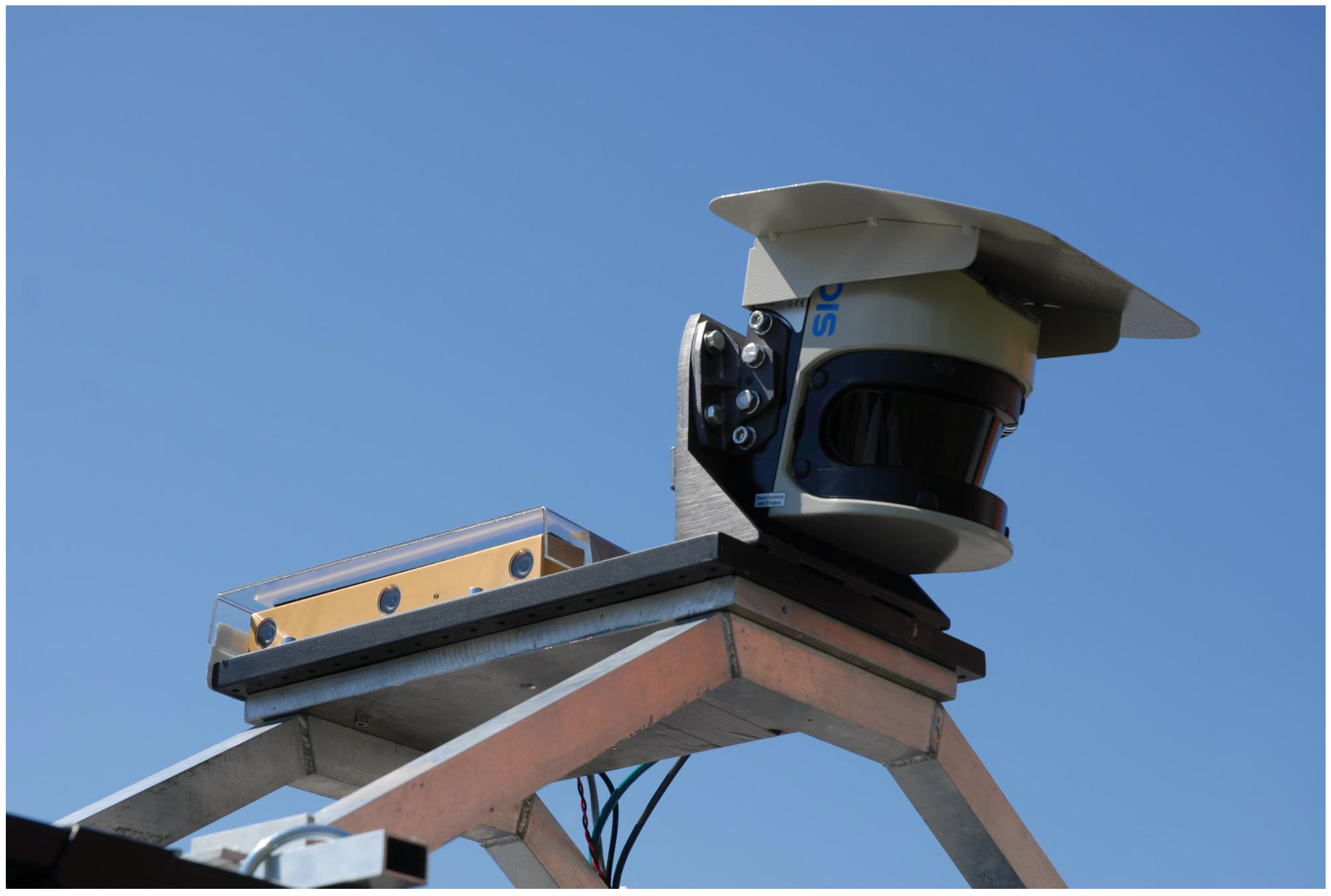
2.3.1. Laser Scanner SICK LMS 511

The SICK LMS 511 laser scanner is a 2D laser scanner (also called line laser scanner). It sends out laser pulses along a horizontal line and records the time until an echo returns for each position in the line. The time is then used to calculate the distance to the object. In this setup, the first echoes were recorded, which means that an echo was recorded when 10% of the presumed signal had been detected. The laser scanner was mounted on a car with 9 degrees declination, in order to get 3D data as the vehicle moves; see Figure 1 and Figure 2. A bird’s eye view of a point cloud is visualized in Figure 3. Data about the laser scanner are presented in

Table 2. SICK LMS 511 data of relevance for the used application (high resolution mode).

Parameter	Value
Beam width	0.68 deg
Separation angle	0.1667 deg
Min distance	0.7 m
Max distance	65 m
Wavelength	950 nm
Scanning frequency	25 Hz
Field of view	190 deg
Point separation @10 m	2.9 cm
Spot size on front screen	1.4 cm
Footprint @10 m	13.3 cm

.

2.3.2. The Chameleon Positioning System

The Chameleon positioning system, developed by FOI [33], has been used for recording the trajectory. Originally, Chameleon was developed to be a highly accurate positioning system for GPS-denied environments, primarily indoors. The high accuracy positioning could increase the security for smoke divers, first responders and soldiers working in unknown buildings. The movement was recorded by an Xsens MTi-G IMU, and visual SLAM using a Point Grey Bumblebee XB3 stereo video was used for reducing the drift. The system mounted on a roof rack with a SICK scanner is shown in Figure 4. At the same time, the movement was tracked, and a map of the surroundings was constructed. Mapping and tracking capacity was sufficient for positioning of a person, but there was some noise in the signal. The system had some drift as a result of the noise. Figure 5 describes a track that should be a closed loop, but it was not.

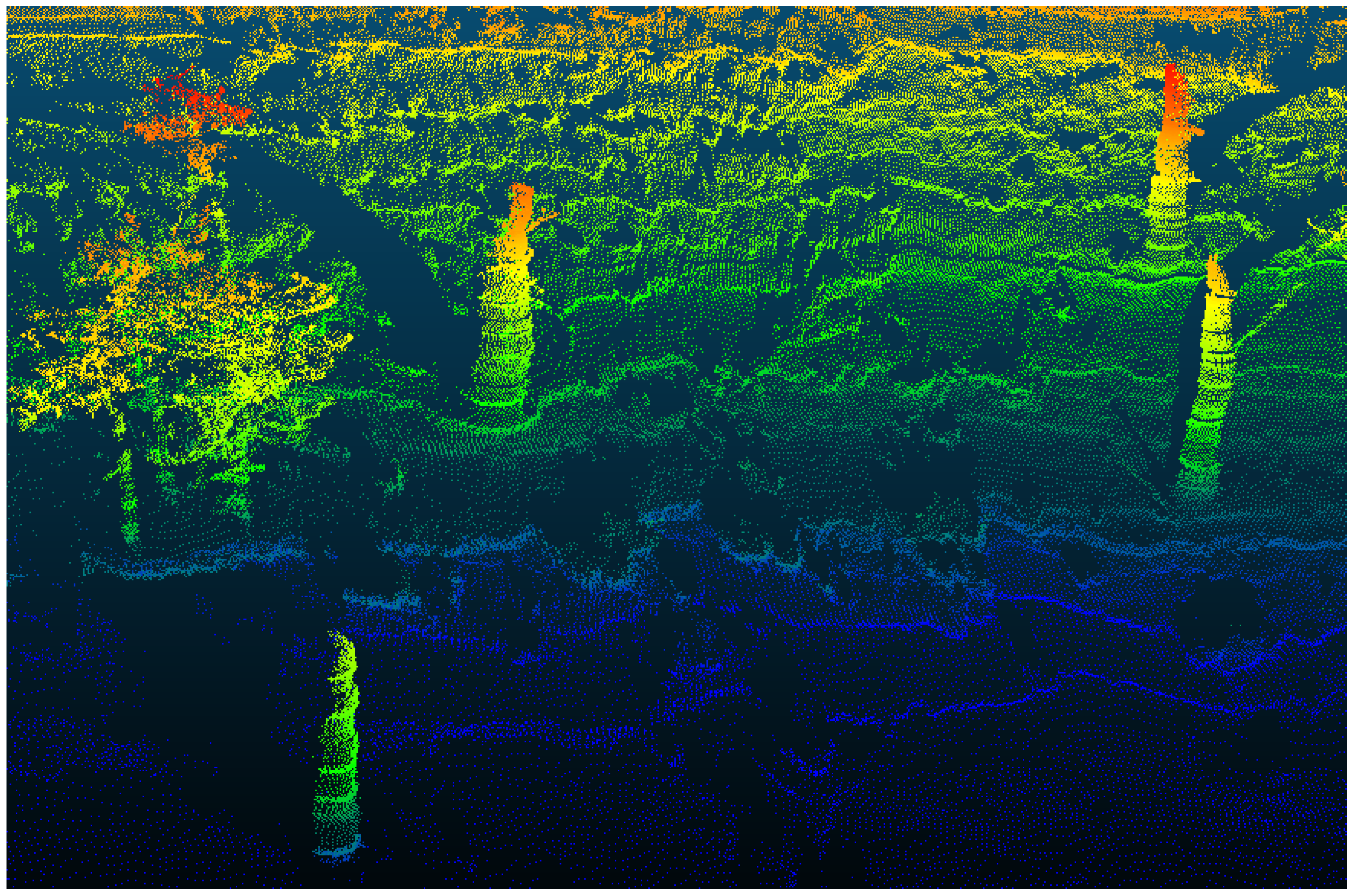
2.3.3. 3D Point Cloud

A 3D point cloud was calculated using the Chameleon trajectory and the distance and angular data from the SICK laser scanner.

For each line:

• Transform from polar coordinates in the sensor system to Cartesian coordinates.
• Rotate the sensor coordinates according to the inclination.
• Rotate the sensor coordinates according to the Chameleon rotation.
• Translate the sensor coordinates to the Chameleon position.
• Store points in a coordinate system originating in the starting point.

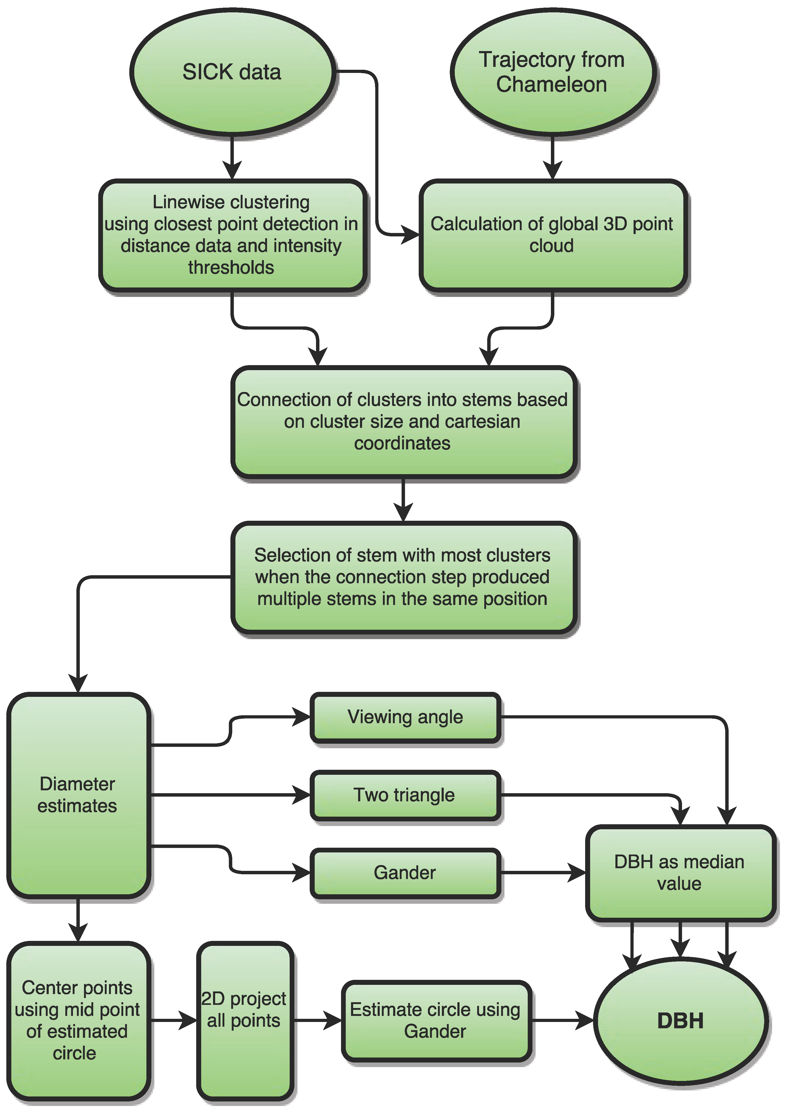
2.3.4. Tree Extraction and DBH Estimation

Since the recorded trajectories have levels of noise that obviously disturb the point cloud quality, the data have been mostly processed line-wise as two-dimensional data. The 3D information has only been used for localization purposes, to connect different clusters into stems and to get the stem positions. A flow chart of the process is presented in Figure 6, and further details are described in this section.

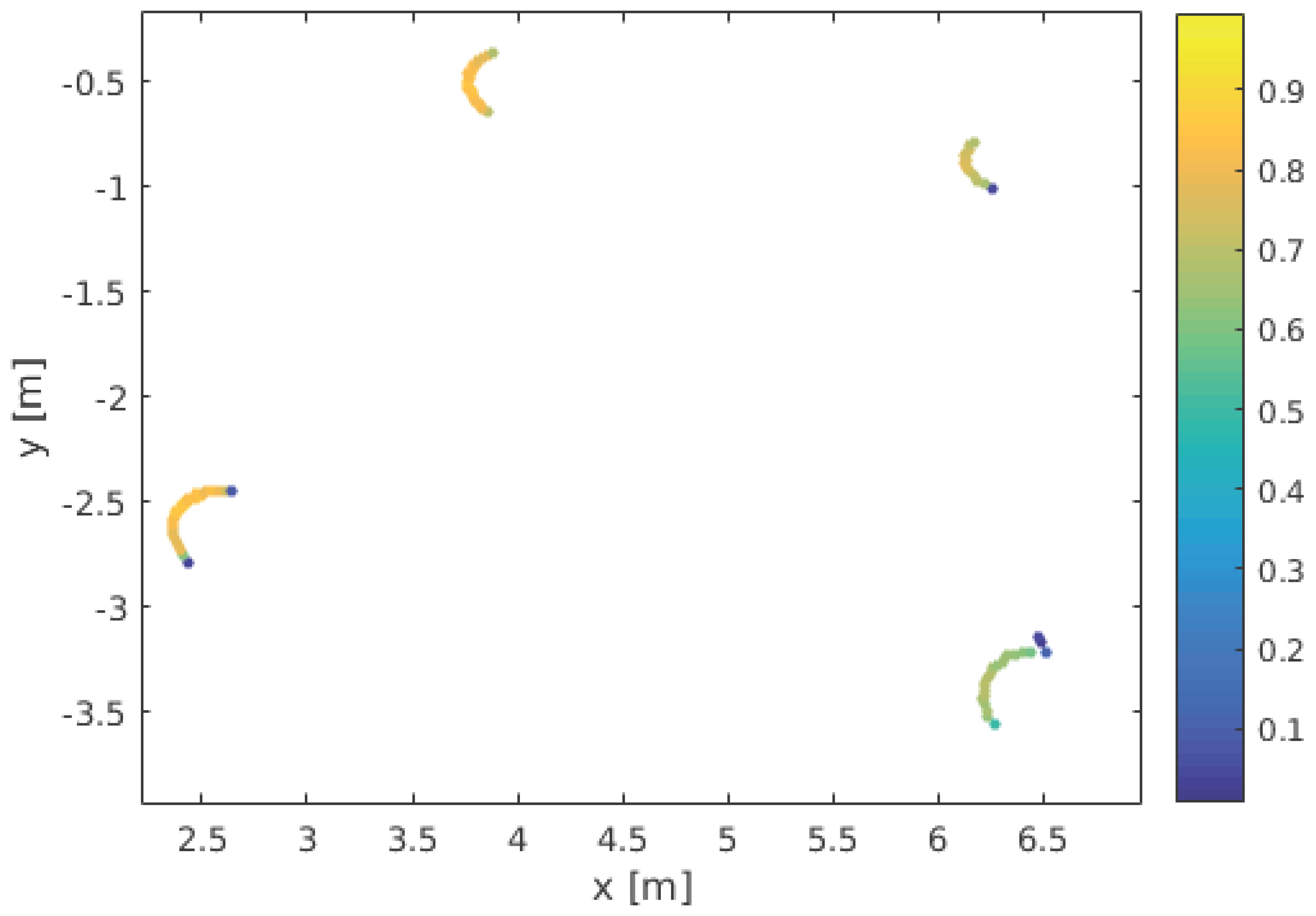
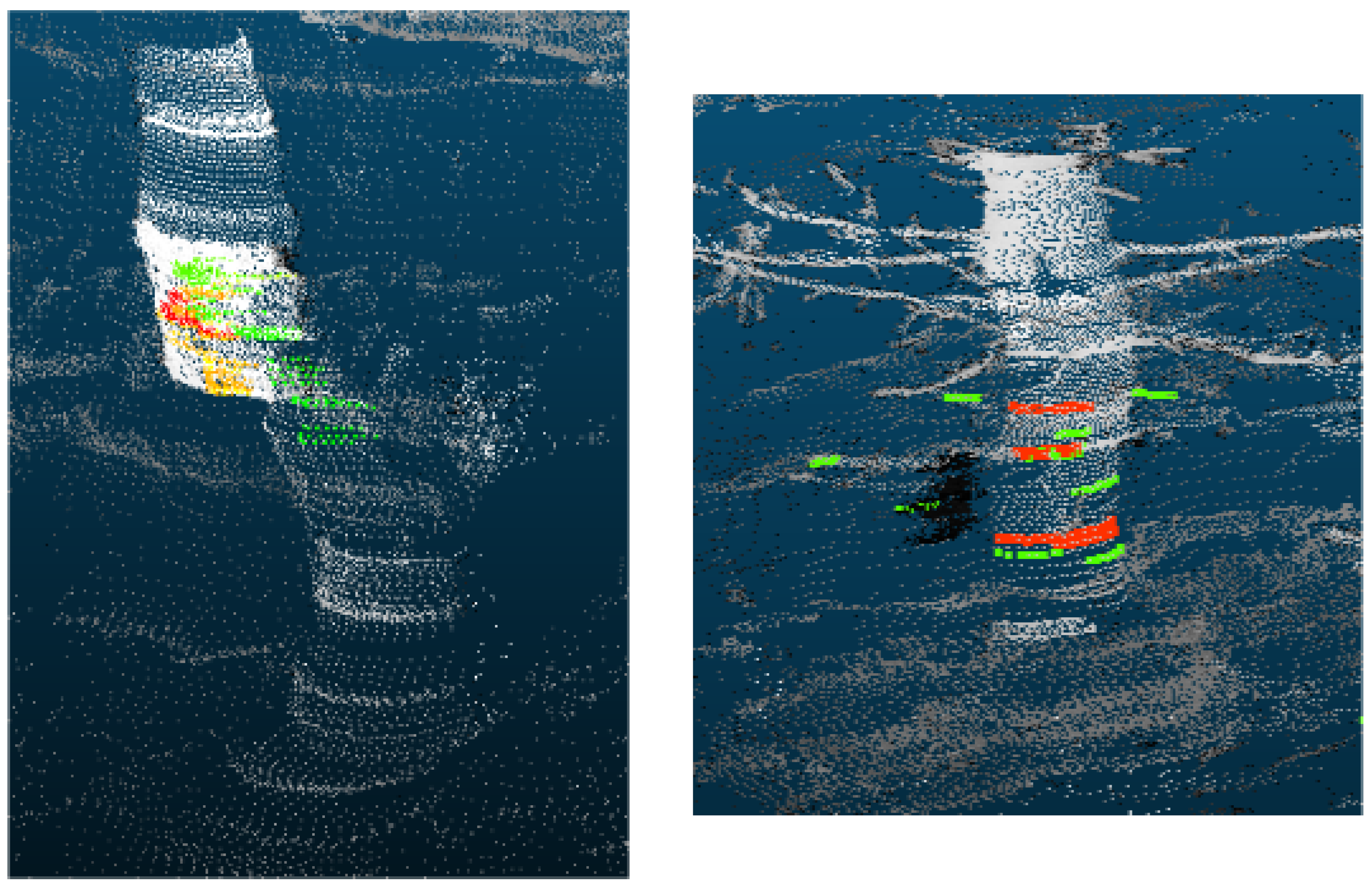
Clustering and Connection

There is a well-known problem, as mentioned above, with circle fitting of 2D line laser scanner data. The origin of the problem is the physical properties of the laser pulse, which causes the echo to be recorded too early, and the described circle will have a larger radius than the object. In this case, with a SICK LMS 511, the footprint of each laser pulse is 13 cm at a 10-m distance, and the separation between the pulses is 3 cm. That implies that four pulses will be overlapping (Figure 7). At the edges of a stem, a phenomenon will occur where first echoes will be recorded for pulses that only touch the stem. Since the laser scanner will register that echo as corresponding to the midpoint of the beam at an angle outside the stem, the stem will appear wider in the point cloud than in reality. In Figure 8, Figure 9 and Figure 10, the effect in terms of point intensity is shown. The points on the edges have much lower intensity, because only a small part of the pulses is reflected. The intensity drops for the outermost points clustered as stem points by a clean distance criterion.

For each line of SICK data:

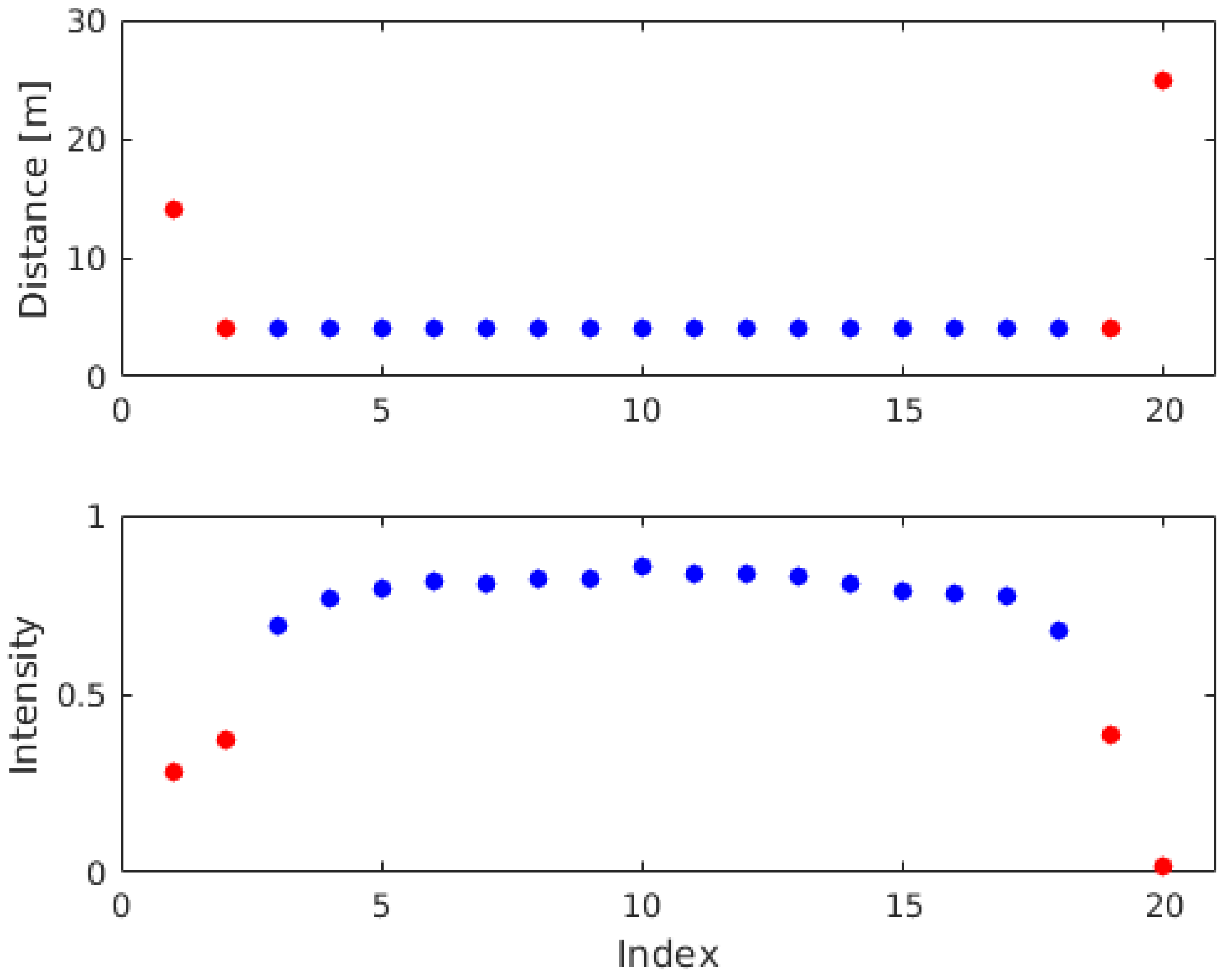
• Trees are detected line-wise in the SICK distance data by detecting negative peaks (shortest distances) that have between 5 and 300 points and are separated with a minimum of 3 points from the next peak.
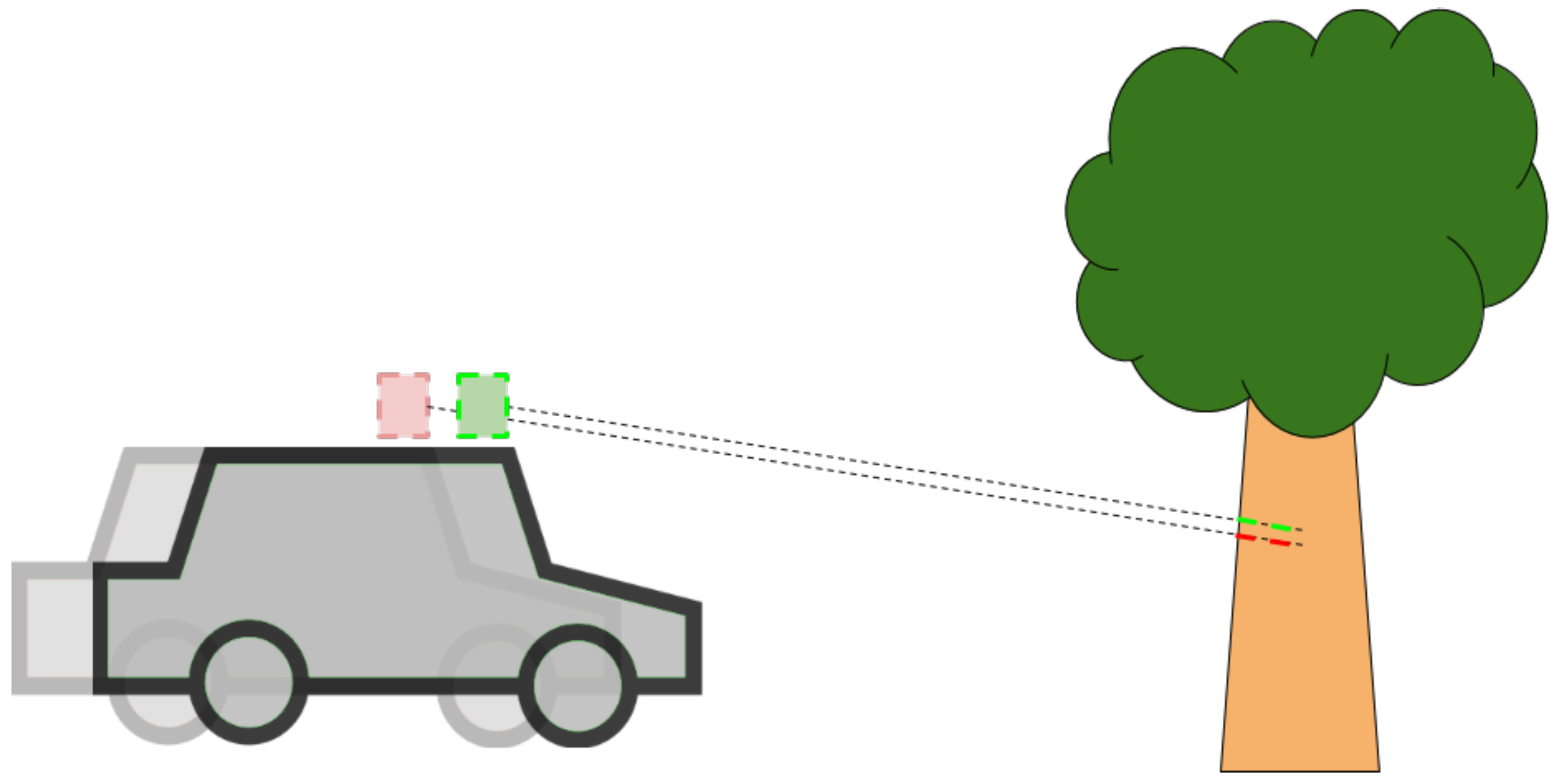
• For each peak, the intensity value of the peak point is saved as a seed point, and then, points to the left and the right are included in the cluster until

  (a)

  the intensity dips under 0.7 times the seed point intensity, or

  (b)

  the difference in distance from the scanner to two neighboring points is larger than 5 cm. A larger distance difference implies that the echo was not returned from the same stem.

• For each cluster where the z-coordinate (height) is within an interval around breast height ($1.3\pm 0.75$ m) in the scanner coordinate system,

  (a)

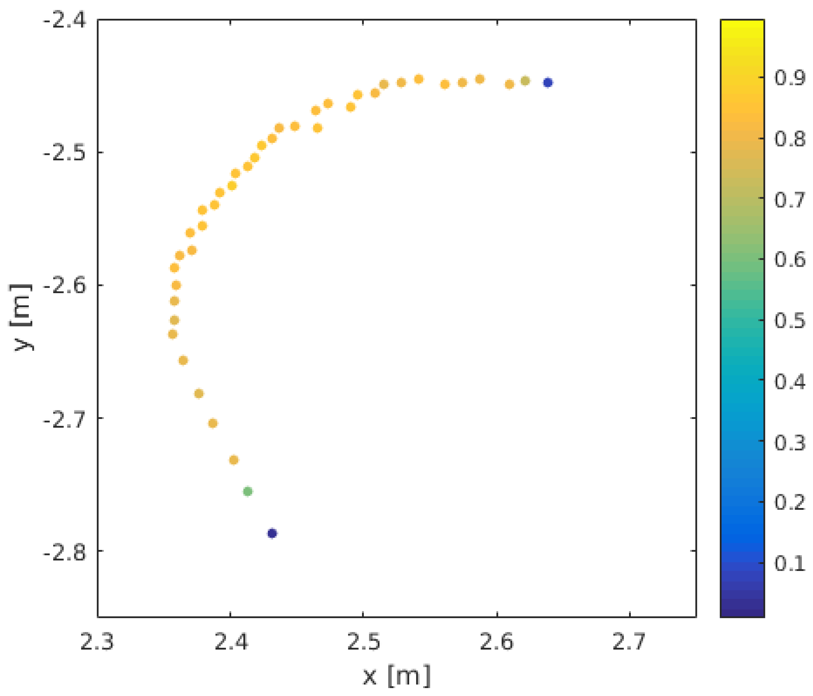
  For the cluster points, a circle fit is done. If the radius is between 3 cm and 50 cm and all of the residuals to the circle are smaller than 4 cm, the cluster is kept.

  (b)

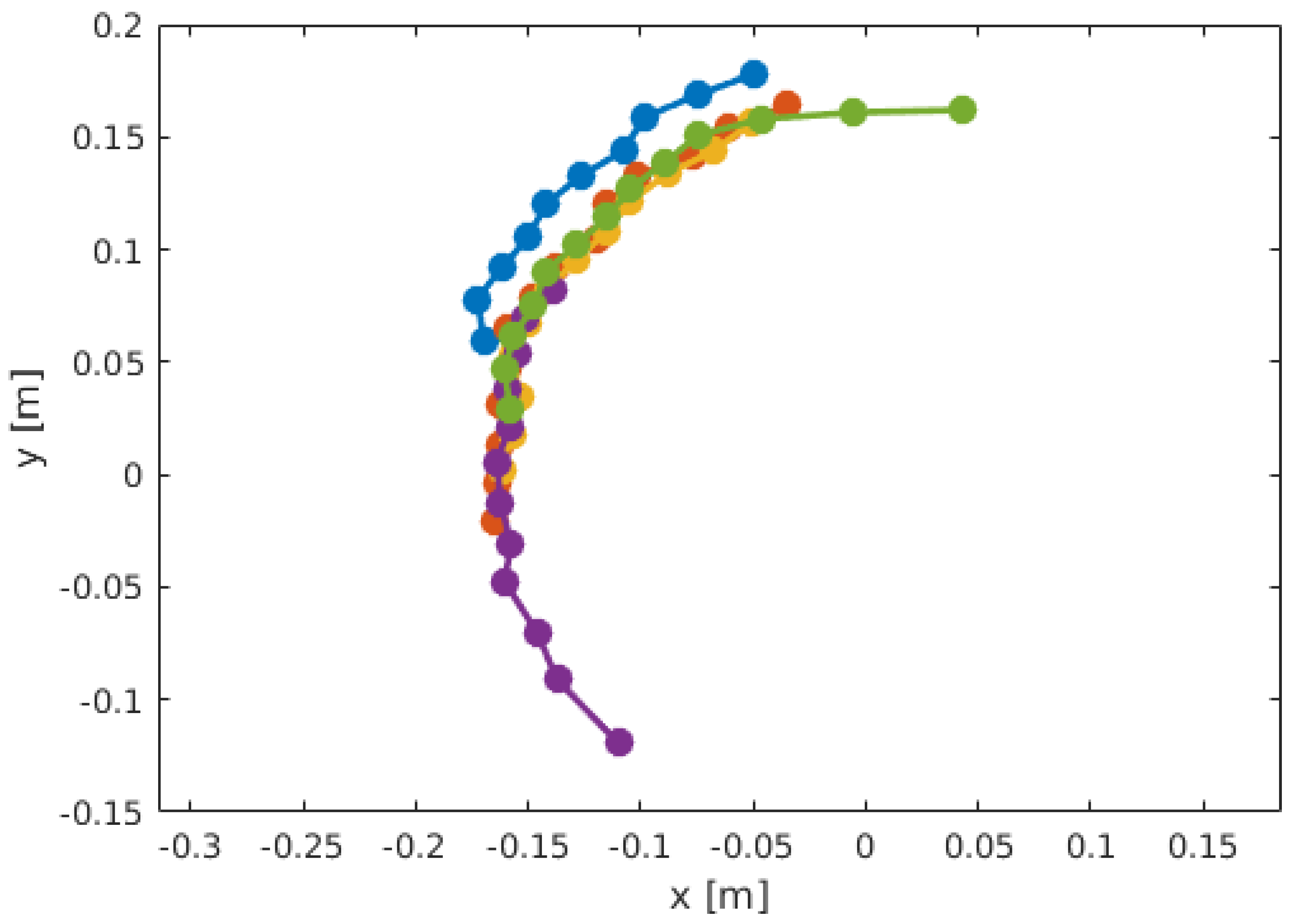
  For each accepted cluster, the Cartesian coordinates are extracted from the point cloud.

  (c)

  Compare to the set of stems. The last cluster to be included in each stem, the top circle, is used as the reference. Include the cluster in a stem if:

  • The x/y-coordinate of the fitted circle is within 10 cm of the top circle of the stem.
  • The radius of the fitted circle is within 4 cm of the top circle of the stem.
  • The line index of the clusters endpoints is close enough to the index of the top circle (Movement 1 index/line number difference is allowed).

  (d)

  Otherwise, a new stem is established from the cluster.

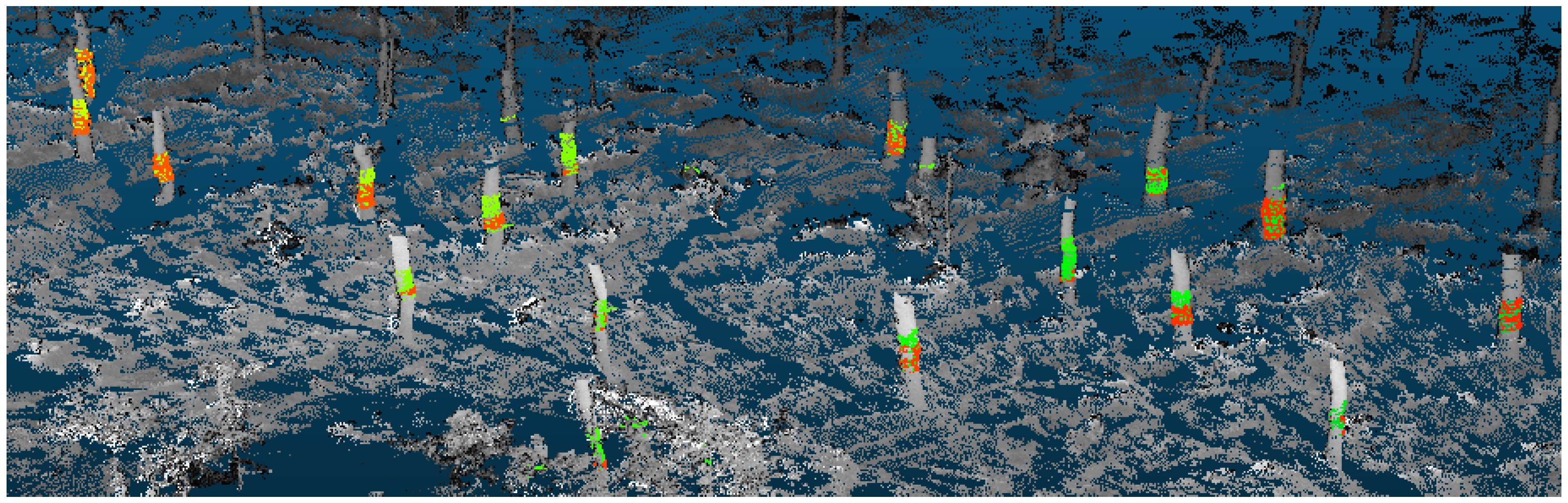
Post-Processing

Since occlusions, such as branches and similar, can cause incomplete clusters of different sizes to occur, there can be multiple stems at the same location in the set of stems. Therefore, the best stem is extracted by majority vote in the following way:

• For all stems, calculate the mean position
• For each stem:

  (a)

  Calculate the distance to all other stems

  (b)

  For stems within a 1-m horizontal distance of the processed stem, select the stem containing the most clusters.

  (c)

  Remove the stem clusters from the set of unprocessed stems.

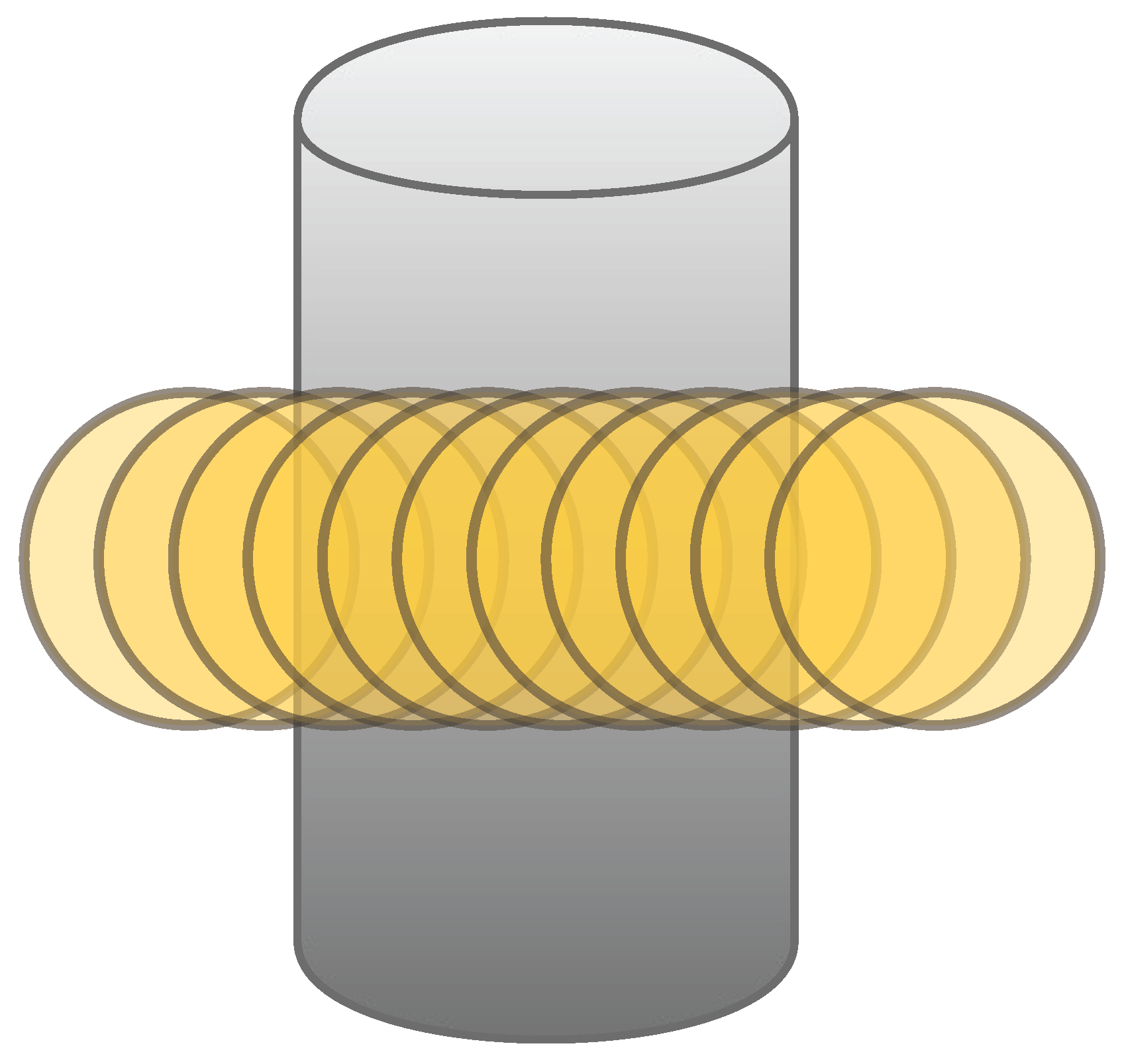
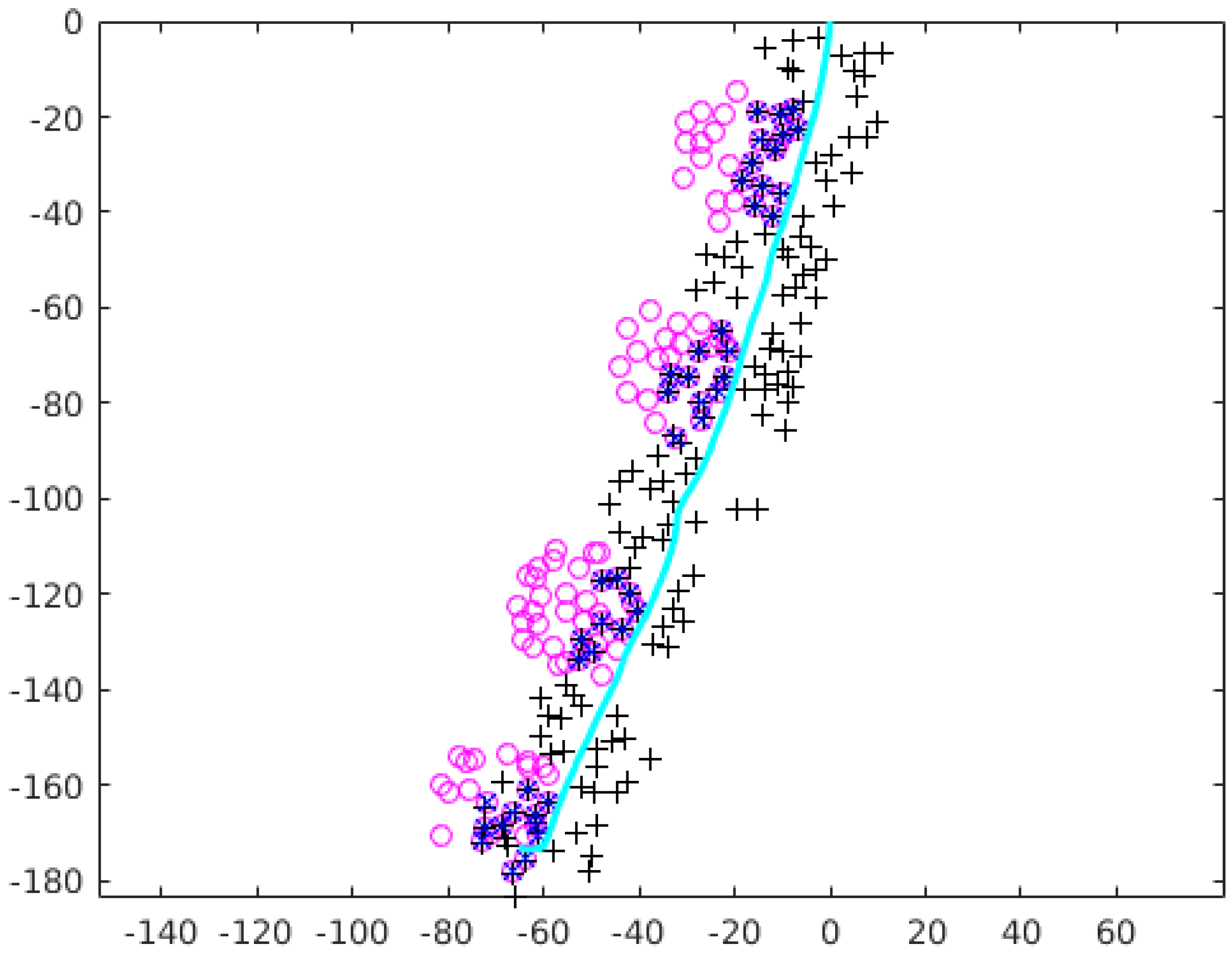
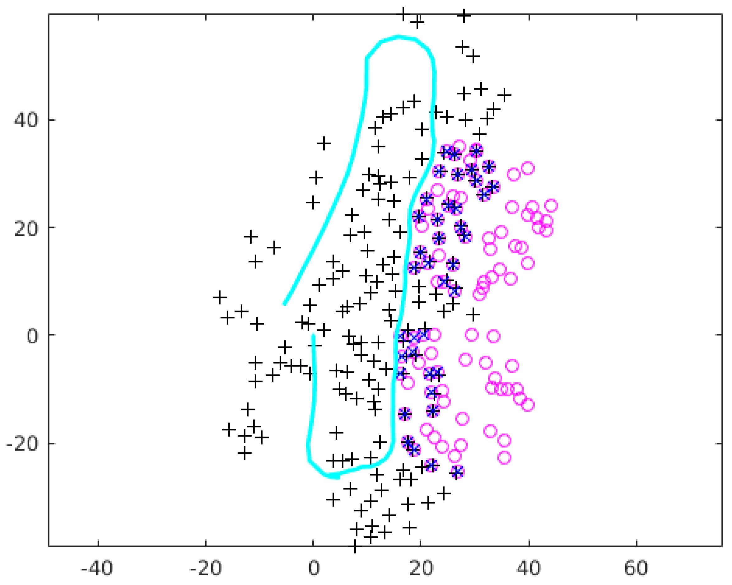
Finding Breast Height in the Point Cloud

Breast height is, for forest measurements purposes, defined as 1.3 m over the germinate point of the tree. This point is often difficult to determine and so was the ground level in this point cloud. Here, we have used the scan-lines at the lower part of the stem within 1.3 ± 0.75 meters above the ground in the scanner coordinate system for the estimation of diameter at breast height. Since a stem taper of approximately 1 cm/m can be estimated for Norway spruce [19] and we assume that the taper of Scots pine is similar, so the coarse estimation of breast height would induce relatively small errors.

DBH Estimation

DBH has been estimated by an assortment of methods to compare the performance of the different algorithms.

The first approach was to estimate the diameter for each line on the stem and then use the median of these values as DBH. Circle fit using Ganders’ direct method (Gand) [34] and two trigonometric methods were implemented. The trigonometric methods, called the viewing angle method (VA) and the two triangle method (2T), are described in [20]. They use the number of points in a cluster, the known angular resolution of the laser scanner and either the distance to the midpoint of the cluster (VA) or the distance to the edge points of the cluster (2T).

The second approach was to use the feature that different scan lines were gathered from different points of view. Then, the points were distributed on a larger part of the circumference of the stem than the points from a single scan line, and a circle fit would be less sensitive to errors in the end points; see Figure 11. For each stem, all of the clusters’ points were centered using the midpoint of a line-wise circle estimated by Ganders’ direct method. Then, the set of points were 2D projected, and to these points, the diameter was estimated using Ganders’ direct method (2DGand).

Gauss–Newton circle fit [35] was also tested, both using the median value and 2D projection for stem estimates. Gauss–Newton performed well in many cases, but if the point dataset is too noisy, the convergence problem occurs, and some stems obtained unrealistic results. Hence, the results became difficult to compare, and we decided not to include the results from the Gauss–Newton method.

2.3.5. Evaluation

The results were compared to the field data. Since the field data were collected on the sides of the track, only a small part of the field data and the MLS data overlaps. For the calculation of bias and RMSE (root mean squared error), all field trees possible to match to the detected trees have been used. Omission and commission error is based on the trees within 10 m of the trajectory. The field data have been compared to visual inspection of the point cloud, and it was found that a few trees were missing in the field data. The missing trees have been manually added for the omission and commission calculation, but since the DBH is unknown, they have not been included in the evaluation of diameter estimation.

3. Results

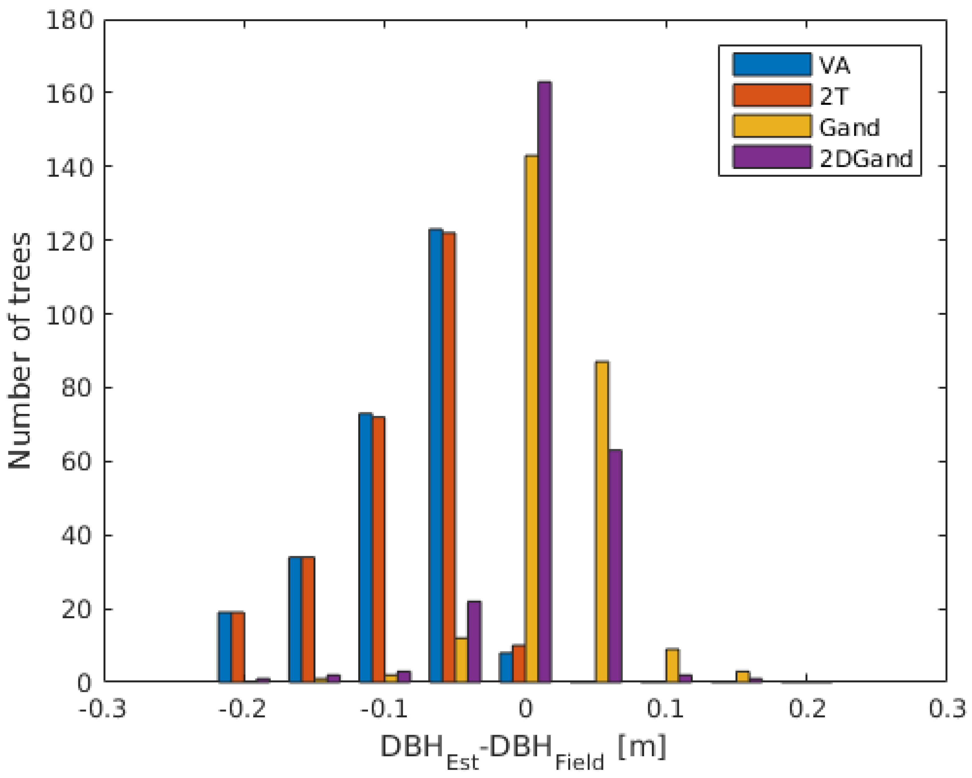
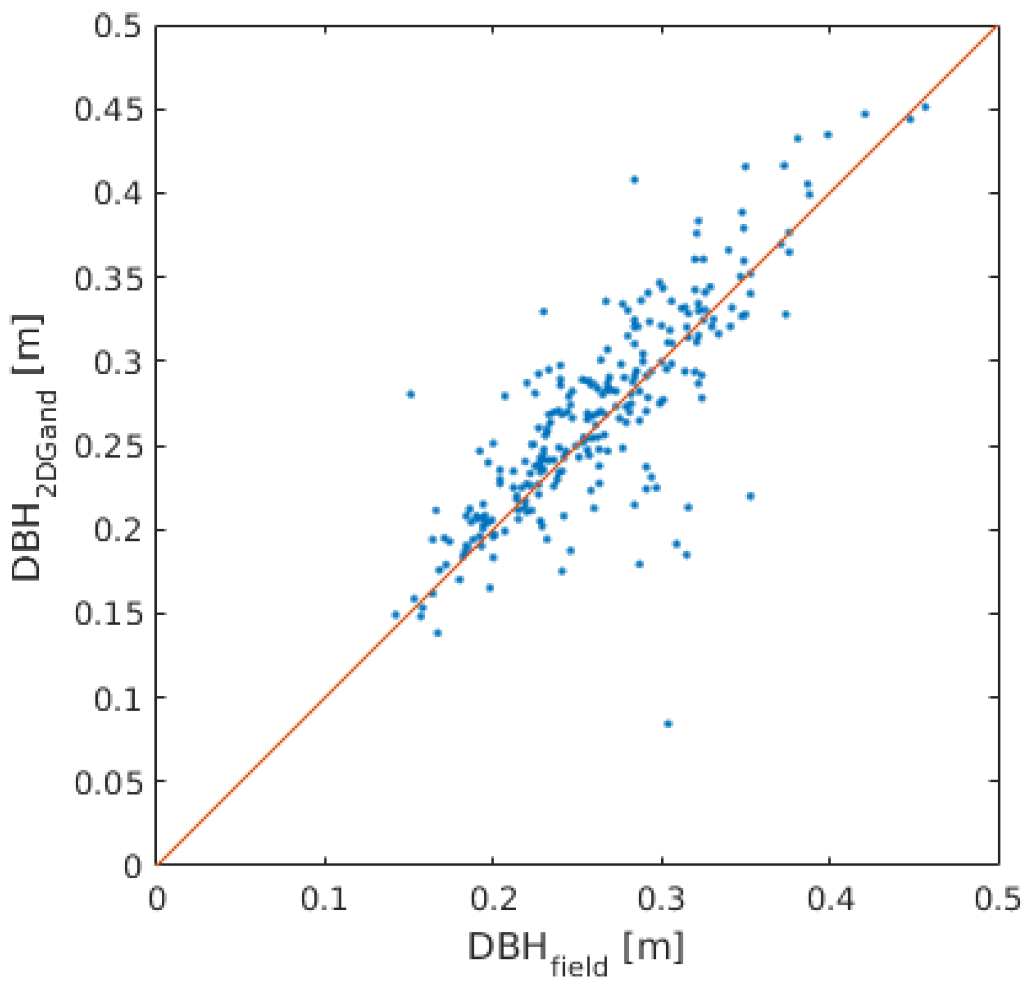
3.1. Diameter Estimation

Four different methods for estimation of diameter at breast height were tested and compared. Results in terms of bias, root mean squared error (RMSE), relative bias (rBias) and relative RMSE (rRMSE) are calculated and presented in

Table 3. Bias, RMSE, relative bias and relative RMSE (rRMSE) of the various estimators on the different sites. Ganders’ direct method on centered and 2D projected points (2DGand) performed best. The median value of Ganders’ direct method (Gand) also performed well.

		2T	VA	Gand	2DGand
Älvan	Bias (m)	−0.086	−0.085	0.012	0.001
	RMSE (m)	0.097	0.096	0.027	0.032
	rBias (%)	−32.68	−32.42	4.50	0.30
	rRMSE (%)	36.95	36.74	10.32	12.35
Sonstorp 1	Bias (m)	−0.086	−0.085	0.029	0.020
	RMSE (m)	0.097	0.097	0.046	0.042
	rBias (%)	−32.07	−31.83	10.81	7.60
	rRMSE (%)	36.42	36.24	17.18	15.90
Sonstorp 2	Bias (m)	−0.095	−0.094	0.010	−0.000
	RMSE (m)	0.108	0.107	0.039	0.035
	rBias (%)	−32.49	−32.24	3.41	−0.14
	rRMSE (%)	37.01	36.82	13.46	12.16
Malmköping 1	Bias (m)	−0.085	−0.085	0.030	0.005
	RMSE (m)	0.096	0.096	0.041	0.035
	rBias (%)	−33.13	−32.92	11.74	2.04
	rRMSE (%)	37.36	37.20	15.77	13.70
Malmköping 2	Bias (m)	−0.079	−0.079	0.025	0.012
	RMSE (m)	0.094	0.093	0.044	0.041
	rBias (%)	−35.43	−35.24	11.16	5.41
	rRMSE (%)	41.84	41.71	19.79	18.22
All	Bias (m)	−0.087	−0.086	0.019	0.006
	RMSE (m)	0.099	0.099	0.038	0.037
	rBias (%)	−33.00	−32.77	7.12	2.30
	rRMSE (%)	37.72	37.54	14.61	13.97

for both the different test areas and summarized for all trees.

Ganders’ method on centered and 2D projected points (2DGand) performs best with relative bias of 2.3% and relative RMSE of 14%. The median value of circle fit with Gander (Gand) is more biased (+7%), but has similar rRMSE (15%). The VA and the 2T methods made gross underestimations with relative bias of −29%. See Figure 12 for a histogram representation of the results and Figure 13 for a scatter plot of the best performing method. The results are similar for all test areas, and no distinct conclusions can be made regarding the influence from various species or whether the terrain is flat or broken. For a comparison, a test was done using point clustering without the intensity criterion; see

Table 4. Bias, RMSE, relative bias and relative RMSE of the various estimators summarized for all sites using a distance-only clustering method. All other used parameters and methods are identical to Table 3.

		2T	VA	Gand	2DGand
All	Bias (m)	−0.072	−0.071	0.042	0.025
	RMSE (m)	0.091	0.091	0.064	0.054
	rBias (%)	−28.50	−28.26	16.76	10.08
	rRMSE (%)	36.06	35.89	25.26	21.34

for the results summarized for all test sites. All other parts of the code were identical. With this setup, the lowest performing methods (VA, 2T) gave slightly better results, and the best performing methods (Gand, 2DGand) gave much worse results. Keeping the intensity criterion and using 2DGand gave the best results in total.

The worst outliers in terms of DBH estimation (overestimation by a factor of 1.85, respectively underestimation by a factor of 0.27) are identified in the point cloud; see Figure 14. The overestimated outlier is a spruce with many branches occluding the stem, and only a few lines have been used for the DBH estimation. The underestimated outlier is a stem that appears to be both curved and clipped due to errors in the positioning system. It is located at the end of a track, and the large positioning error may be influenced by the car stopping and turning around.

3.2. Tree Detection

In Figure 15, the detection behavior is visualized, with the points used for DBH estimation being color marked. The mean distance to detected trees was about 9 m, and the maximum distance was almost 15 m for all test sites. The tree detection rate in terms of omission and commission errors has been evaluated within 10 m from the trajectory and is presented in

Table 5. Number of found trees, number of field trees, number of trees matched to field data, number of field trees within 10 m, number of matched trees within 10 m and commission and omission errors within 10 m. Results are based on the complete method using the intensity criterion for clustering.

Test Site	Found Trees Total	Field Trees Total	Matched Trees	Field Trees D < 10 m	Matched Trees D < 10 m	Commission D < 10 m	Omission D < 10 m
Älvan	369	194	77	93	62	0	31
Sonstorp 1	168	101	39	51	33	0	19
Sonstorp 2	163	152	62	62	48	0	14
Malmköping 1	170	85	34	38	27	0	11
Malmköping 2	156	117	45	49	38	2	11

.

Figure 16, Figure 17, Figure 18, Figure 19 and Figure 20 display maps over the detected trees and the field trees for all of the test areas. The drift in the positioning system was obvious on tracks where the same path was traversed forward and then back. The path was missed by several meters in some cases. It was not possible then to match the trees to field data. Therefore, only one direction has been used for the evaluation of the Sonstorp 2 and Malmköping 2 areas.

4. Discussion

In this article, we have presented a new system of methods for the estimation of DBH from a prototype of a mobile laser scanning system. A 2D laser scanner was mounted facing forward, tilted nine degrees downwards, on a car, and the trajectory was recorded using a combination of inertial navigation and visual SLAM. A 3D point cloud had been constructed from the laser scanning data, the trajectory and the orientation of the scanner. High-precision positioning is a difficult problem to solve in forests, and hence, the trajectory included both drift and noise that made the point cloud unsuitable for processing with established methods for 3D laser scanning point clouds.

We have treated the point cloud line-wise, to reduce the effects of the positioning error on the DBH estimation. Some insights have been made about the errors in laser scanning points on inclined surfaces, and a new clustering method using an intensity criterion has resulted in clusters of stem points that are more suitable for the circle fit. The moving sensor gave measurements from more than one view on the stem, and measurements on a larger part of the circumference could be used for diameter estimation using the circle fit.

The positioning errors of the sensor affect the 3D point cloud, but since the positioning only was used in this study for the connection of clusters into stems and for the estimation of the tree positions, they do not affect the DBH estimation directly. Some trees have been omitted due to the drift in the positioning system, which made some trees appear cut into pieces or severely inclined in the point cloud.

A common approach to clustering of 3D point clouds to detect tree trunks is to calculate normals to each point using its neighborhood as a plane and a smoothness constraint to determine whether they are included in the cluster or not. In this kind of MLS point cloud, the artifacts from the positioning error with translated lines have given many stems a wave-like structure, and the normal directions of the points on the stem surface can be too irregular for the smoothness constraint to succeed. The line-wise approach removed the need for smooth transitions of the normal directions, and this problem was avoided.

The intensity criterion for clustering of stem points have filtered away the measurements with large errors on the flanks of the trees. This method gives sufficient input point sets for circle fit, since the points with the largest position errors are not included. A removal of the intensity criterion increases the errors with circle fit. In earlier works, the use of circle fit on line scanner data has resulted in gross overestimations [20].

For the VA and 2T methods, the diameters have been underestimated by more than 30%. These methods have been favored in earlier works [20,21,36] due to the smaller errors compared to the circle fit. Those methods are affected by the discrete nature of the signal. At a 10-m distance from the sensor, the separation of the measured points is 3 cm. That results in a possible underestimation of up to 6 cm, just due to the point separation. This is not the only reason for the underestimation in this study. When the intensity criterion was removed, the underestimation was reduced, but the assumed overestimation did not occur. Influence from incomplete clusters, which are not filtered away in this implementation, can be the reason for this behavior. Incomplete clusters will appear when the scan line is interrupted, for example by a branch, and a point is measured at a distance too short to be included in the segment. On a stem with many branches, there are many incomplete clusters that include enough points for a circle fit, but since one or both of the edge points are missing, the trigonometric methods fail. On large stems at long distances, a problem may occur with the distance difference criterion of 5 cm for neighboring points, which may be too short of a tolerance distance.

In a point cloud gathered from a single point of view, only points facing the view point are present. This is problematic for circle fit on cylindrical objects, such as trees, since the gathered information represents a sector that is less than half the circumference. The 2D projection of circles from different scan lines, and hence, different scanner positions, increases the sector with information, and the influence of the less accurate flank points with smeared footprints is lower. Ganders’ direct method on 2D projected points performed best, with relative bias of 2.3% (0.6 cm) and relative RMSE of 14% (3.7 cm). The initial study on this dataset, Barth et al. [29], obtained a smaller bias of −1.9% (−0.5 cm), but a larger RMSE of 24% (5.8 cm).

The results are comparable to those of similar methods. In a laboratory setting, Kong et al. [23] measured stem diameters with a bias of 4%. They used multiple scans to reduce the influence from the statistical errors of the sensors, and the resulting sets of points were suitable for the circle fit. From a field experiment, Jutila et al. [21] report a bias of 4%, which is larger than ours, and a relative error of 11%.

Brunner and Gizachew [19] have evaluated their method on basal area estimates, and have not summarized the DBH statistics, but their plot-wise tables indicate a bias of 3.7 cm and an RMSE of 6.8 cm. Dian et al. [22] reports impressive results with an error of 4.29 mm. However, their comparison material consists of artificial measurements on the laser scanner point cloud, which will differ from field measurements, since it includes the uncertainty in the laser points.

The result that the circle fit performs best is contradictory to Ringdahl et al. [20], Jutila et al. [21] and Hellstrom et al. [36]. The problem with large errors in the edge points has been pointed out by Ringdahl et al. [20]. They have improved a trigonometric algorithm to adjust the stem diameter estimations. Our approach to use the intensity criterion to not include the points partly reflected by the stem in the cluster has given the circle fit methods a set of points that are good enough to succeed. On the other hand, the trigonometric methods earlier preferred produce underestimations when the edge points are removed.

Liang et al. [37] have measured a large field plot using a 3D laser scanner mounted on an all-terrain vehicle. Since a 3D laser scanner was used, they were able to use methods developed for stationary TLS point clouds. The reported error for DBH is a bias of −2.52 cm and an RMSE of 2.36 cm, which is smaller than our errors using a line laser scanner.

The positioning of the trees is affected by the drift in the positioning system. To be able to extract a high quality tree map of a forest stand, a more precise way of tracking the trajectory is needed. One way could be to mount the laser scanner and the positioning system in a suspension system that reduces the vibrations and smooths the physical movement. Another possibility, maybe in combination with a suspension system, would be to include the laser scanner data in the SLAM algorithm.

The need for movement to create the 3D environment complicates the system for aiding a harvester operator with decision support. With this configuration of the system, breast height of the trees will be measured at 7.5 m in front of the scanner. A harvester crane can reach trees outside that range and cut unmeasured trees. A steeper declination of the scanner would find breast height closer to the sensor, but also shorten the working range and make the vertical resolution sparser.

Most of the omitted trees are omitted due to one of three reasons.

(1) The tree has several branches in the height of interest (probably spruce), and there are too few clusters that are circle-like with a similar radius on the stem. This problem could be resolved using multiple echoes from the laser scanning, but further signal processing would be needed to extract only echoes from the tree stems.

(2) The tree is occluded by other trees, and the height of interest is never visible from the scanner position. Some of the trees omitted for this reason could probably be found using a multi-line 2D laser scanner scanning in, for example, 16 or 32 lines.

(3) The drift in the positioning system has made the tree too inclined, or it even appears cut into pieces, to be accepted as one tree. A positioning system with higher precision and stability would resolve this problem. Another possible solution would be to include the line-wise-detected stems in the SLAM algorithm.

The results contain two trees as commission errors. They are positioned close to each other at the end of the Malmköping 2 test site. In that position, due to positioning errors, the point cloud contains artifacts that are not manually interpretable as to whether there are trees in that position or not.

MLS data contain two limitations for the estimation of forest statistics on the stand level. Firstly, the pattern of occluded trees must be regarded. A tree at a very short distance can occlude multiple other trees. The other limitation is a possible bias due to the choice of path for the sensor-bearing vehicle. For example, wet areas, rocky terrain or very dense forest may be avoided due to the difficulty of driving there.

5. Conclusions

In this article, we used a number of new methods to enhance the results of automatic DBH estimations from mobile laser scanner data. Firstly, the approach to use the data line-wise for clustering and diameter estimation made the estimation of stem diameter independent of the quality of the trajectory and the co-registered point cloud. Secondly, the clustering of the stems based on an intensity criterion and not only on spatial criteria removed the flank points, which may be positioned outside the stem. The last novelty was the centering and 2D projection of points on the same tree trunk, but from different scanner positions. In that way, points on a larger part of the circumference were gathered. The flank points with larger errors had less influence, and circle fit using Ganders’ direct method performed satisfactorily.

The observations from this study imply that mobile laser scanning using this or similar methods can be practically applicable and used for collecting the status of a forest stand after thinning or for data collection from a moving vehicle.

References

1. Holopainen, M.; Vastaranta, M.; Hyyppä, J. Outlook for the Next Generation’s Precision Forestry in Finland. For. Trees Livelihoods 2014, 5, 1682–1694. [Google Scholar] [CrossRef]
2. Öhman, M.; Miettinen, M.; Kannas, K.; Jutila, J.; Visala, A.; Forsman, P. Tree Measurement and Simultaneous Localization and Mapping System for Forest Harvesters. In Field and Service Robotics; Springer Tracts in Advanced Robotics; Springer (Berlin Heidelberg): Heidelberg, Germany, 2008; pp. 369–378. [Google Scholar]
3. Roßmann, J.; Krahwinkler, P.; Schlette, C. Navigation of mobile robots in natural environments: Using sensor fusion in forestry. J. Syst. Cybern. Inform. 2010, 8, 67–71. [Google Scholar]
4. Thies, M.; Pfeifer, N.; Winterhalder, D.; Gorteb, B.G.H. Three-dimensional Reconstruction of Stems for Assessment of Taper, Sweep and Lean Based on Laser Scanning of Standing Trees. Scand. J. For. Res. 2004, 19, 571–581. [Google Scholar] [CrossRef]
5. Pfeifer, N.; Gorte, B.; Winterhalder, D. Automatic Reconstruction of Single Trees from Terrestrial Laser Scanner Data. In Proceedings of the 20th ISPRS Congress, Istanbul, Turkey, 12–23 July 2004.
6. Pfeifer, N.; Winterhalder, D. Modelling of Tree Cross Sections from Terrestrial Laser Scanning Data with Free-form Curves. Int. Arch. Photogramm. Remote Sens. Spat. Inf. Sci. 2004, XXXVI, 76–81. [Google Scholar]
7. Lindberg, E.; Holmgren, J.; Kenneth, O.; Olsson, H. Estimation of stem attributes using a combination of terrestrial and airborne laser scanning. Eur. J. For. Res. 2012, 131, 1917–1931. [Google Scholar] [CrossRef]
8. Liang, X.; Kankare, V.; Yu, X.; Hyyppä, J.; Holopainen, M. Automated stem curve measurement using terrestrial laser scanning. IEEE Trans. Geosci. Remote Sens. 2014, 52, 1739–1748. [Google Scholar] [CrossRef]
9. Olofsson, K.; Holmgren, J.; Olsson, H. Tree Stem and Height Measurements Using Terrestrial Laser Scanning and the RANSAC Algorithm. Remote Sens. 2014, 6, 4323–4344. [Google Scholar] [CrossRef]
10. Treemetrics. Available online: http://www.treemetrics.com (accessed on 13 September 2016).
11. Hackenberg, J.; Wassenberg, M.; Spiecker, H.; Sun, D. Non Destructive Method for Biomass Prediction Combining TLS Derived Tree Volume and Wood Density. For. Trees Livelihoods 2015, 6, 1274–1300. [Google Scholar] [CrossRef]
12. Liang, X.; Kankare, V.; Hyyppä, J.; Wang, Y.; Kukko, A.; Haggrén, H.; Yu, X.; Kaartinen, H.; Jaakkola, A.; Guan, F.; et al. Terrestrial laser scanning in forest inventories. ISPRS J. Photogramm. Remote Sens. 2016, 115, 63–77. [Google Scholar] [CrossRef]
13. Hauglin, M.; Astrup, R.; Gobakken, T.; Næsset, E. Estimating single-tree branch biomass of Norway spruce with terrestrial laser scanning using voxel-based and crown dimension features. Scand. J. For. Res. 2013, 28, 456–469. [Google Scholar] [CrossRef]
14. Kankare, V.; Holopainen, M.; Vastaranta, M.; Puttonen, E.; Yu, X.; Hyyppä, J.; Vaaja, M.; Hyyppä, H.; Alho, P. Individual tree biomass estimation using terrestrial laser scanning. ISPRS J. Photogramm. Remote Sens. 2013, 75, 64–75. [Google Scholar] [CrossRef]
15. Pueschel, P.; Newnham, G.; Rock, G.; Udelhoven, T.; Werner, W.; Hill, J. The influence of scan mode and circle fitting on tree stem detection, stem diameter and volume extraction from terrestrial laser scans. ISPRS J. Photogramm. Remote Sens. 2013, 77, 44–56. [Google Scholar] [CrossRef]
16. Krooks, A.; Kaasalainen, S.; Hakala, T.; Nevalainen, O. Correction of Intensity Incidence Angle Effect in Terrestrial Laser Scanning. ISPRS Ann. Photogramm. Remote Sens. Spat. Inf. Sci. 2013, II-5/W2, 145–150. [Google Scholar] [CrossRef]
17. Kelbe, D.; Romanczyk, P.; van Aardt, J.; Cawse-Nicholson, K. Reconstruction of 3D tree stem models from low-cost terrestrial laser scanner data. In Proceedings of the SPIE 8731, Laser Radar Technology and Applications XVIII, 2013, Baltimore, MD, USA, 29 April–3 May 2013. [CrossRef]
18. Kelbe, D.; van Aardt, J.; Romanczyk, P.; van Leeuwen, M.; Cawse-Nicholson, K. Single-Scan Stem Reconstruction Using Low-Resolution Terrestrial Laser Scanner Data. IEEE J. Sel. Top. Appl. Earth Obs. Remote Sens. 2015, 8, 3414–3427. [Google Scholar] [CrossRef]
19. Brunner, A.; Gizachew, B. Rapid detection of stand density, tree positions, and tree diameter with a 2D terrestrial laser scanner. Eur. J. For. Res. 2014, 133, 819–831. [Google Scholar] [CrossRef]
20. Ringdahl, O.; Hohnloser, P.; Hellström, T.; Holmgren, J.; Lindroos, O. Enhanced Algorithms for Estimating Tree Trunk Diameter Using 2D Laser Scanner. Remote Sens. 2013, 5, 4839–4856. [Google Scholar] [CrossRef]
21. Jutila, J.; Kannas, K.; Visala, A. Tree Measurement in Forest by 2D Laser Scanning. In Proceedings of the 2007 IEEE International Symposium on Computational Intelligence in Robotics and Automation, Jacksonville, FL, USA, 20–23 June 2007.
22. Wang, D.; Liu, J.; Wang, J. Diameter Fitting by Least Square Algorithm Based on the Data Acquired with a 2-D Laser Scanner. Procedia Eng. 2011, 15, 1560–1564. [Google Scholar]
23. Kong, J.; Ding, X.; Liu, J.; Yan, L.; Wang, J. New Hybrid Algorithms for Estimating Tree Stem Diameters at Breast Height Using a Two Dimensional Terrestrial Laser Scanner. Sensors 2015, 15, 15661–15683. [Google Scholar] [CrossRef] [PubMed]
24. Brach, M.; Zasada, M. The effect of mounting height on GNSS receiver positioning accuracy in forest conditions. Croat. J. For. Eng. 2014, 35, 245–253. [Google Scholar]
25. Antonio, A. GNSS/INS Integration Methods; University of Calgary: Calgary, AB, Canada, 2010. [Google Scholar]
26. Dissanayake, M.W.M.G.; Newman, P.; Clark, S.; Whyte, H.F.W.; Csorba, M. A solution to the simultaneous localization and map building (SLAM) problem. IEEE Trans. Rob. Autom. 2001, 17, 229–241. [Google Scholar] [CrossRef]
27. Pesyna, K.M., Jr.; Heath, R.W., Jr.; Humphreys, T.E. Centimeter positioning with a smartphone-quality GNSS antenna. In Proceedings of the 27th International Technical Meeting of the Satellite Division of the Institute of Navigation (ION GNSS+ 2014), Tampa, FL, USA, 8–12 September 2014; pp. 1568–1577.
28. Chen, Y.; Zhao, S.; Farrell, J.A. Computationally Efficient Carrier Integer Ambiguity Resolution in Multiepoch GPS/INS: A Common-Position-Shift Approach. IEEE Trans. Control Syst. Technol. 2015, 24, 1541–1556. [Google Scholar] [CrossRef]
29. Barth, A.; Willén, E.; Holmgren, J.; Olofsson, K.; Bilock, E.; Engström, P.; Larsson, H.; Rydell, J. Mobilt Mätsystem för Insamling av Träd- och Beståndsdata; Technical Report; Forestry Research Agency of Sweden: Skogforsk, Sweden, 2014. [Google Scholar]
30. Haglöf. Available online: http://www.haglofcg.com (accessed on 31 May 2016).
31. Nilsson, M.; Nordkvist, K.; Jonzén, J.; Lindgren, L.; Axensten, P.; Wallerman, J.; Egberth, M.; Larsson, S.; Nilsson, L.; Eriksson, J.; et al. A Nationwide Forest Attribute Map of Sweden Derived using Airborne laser scanning data and field data from the national forest inventory. In Proceedings of the SilviLaser 2015, La Grande Motte, France, 28–30 September 2015; pp. 211–213.
32. Swedish Forest Agency. Available online: http://www.skogsstyrelsen.se/Aga-och-bruka/Skogsbruk/Karttjanster/Laserskanning/ (accessed on 23 August 2016).
33. Rydell, J.; Emilsson, E. Chameleon: Visual-inertial indoor navigation. In Proceedings of the Position Location and Navigation Symposium (PLANS), 2012 IEEE/ION, Myrtle Beach, SC, USA, 23–26 April 2012; pp. 541–546.
34. Gander, W.; Golub, G.H.; Strebel, R. Least-squares fitting of circles and ellipses. BIT Numer. Math. 1994, 34, 558–578. [Google Scholar] [CrossRef]
35. Börlin, N.; Grussenmeyer, P. Bundle Adjustment with and without Damping. Photogramm. Rec. 2013, 28, 396–415. [Google Scholar] [CrossRef]
36. Hellström, T.; Hohnloser, P.; Ringdahl, O. Tree Diameter Estimation Using Laser Scanner; Technical Report UMINF 12.20; Umeå University: Umeå, Sweden, 2012. [Google Scholar]
37. Liang, X.; Hyyppä, J.; Kukko, A.; Kaartinen, H.; Jaakkola, A.; Yu, X. The Use of a Mobile Laser Scanning System for Mapping Large Forest Plots. IEEE Geosci. Remote Sens. Lett. 2014, 11, 1504–1508. [Google Scholar] [CrossRef]
Figure 1. SICK LMS 511 line laser scanner mounted on a terrain car together with the Chameleon positioning system. The laser scanner is mounted facing forward, with an declination of 9 degrees.
Forests 07 00206 g001
Figure 2. As the vehicle moves, a 3D point cloud of the surroundings can be constructed using the 2D laser scanner distance data in combination with the position and the orientation of the sensor.
Forests 07 00206 g002
Figure 3. Bird’s eye view of a point cloud colored by line number. Blue, low number; red, high number. Every stem casts a shadow over a curved area, which is occluded from view.
Forests 07 00206 g003
Figure 4. SICK scanner and the Chameleon positioning system mounted on a roof rack. The SICK scanner is facing forward with 9 degrees of declination, and the Bumblebee camera is facing sideways.
Forests 07 00206 g004
Figure 5. 3D trajectory from Chameleon on Sonstorp 1. The drift in the system is visible, since these data were recorded from a closed loop.
Forests 07 00206 g005
Figure 6. Flowchart.
Forests 07 00206 g006
Figure 7. Stem at 10 m. Diameter 20 cm; the angle separation between beam centers of 0.17 degrees gives a 2.9-cm separation on the stem; beam divergence 0.68 degrees + spot size 1.4 cm equals a 13.3-cm footprint.
Forests 07 00206 g007
Figure 8. Four stem point clusters from one line of SICK data after 3D calculation projected on the ground plane. The points are colored according to normalized intensity. The endpoints of the clusters based on distance criterion have lower intensity (blue).
Forests 07 00206 g008
Figure 9. Edge points. A stem point cluster where the end points have lower intensity (blue). The blue points do not lie on the same circle as the yellow ones; they are slightly outside.
Forests 07 00206 g009
Figure 10. Blue points clustered as stem by intensity, red points as not stem. One point on each flank outside the stem cluster is at the same distance as the stem cluster and should by distance clustering be classified as stem. x-axis: point index in the cluster.
Forests 07 00206 g010
Figure 11. Overlapping point clusters from different scan lines gives a larger part of the stems circumference to which to fit a circle.
Forests 07 00206 g011
Figure 12. Histogram over DBH Est - DBH Field for all matched trees. Ganders’ direct method on 2D projected points (2DGand) has the smallest bias. The trigonometric methods VA (viewing angle) and 2T (two triangle) underestimate systematically.
Forests 07 00206 g012
Figure 13. Scatter plot of DBH estimated by the most successful method, 2DGand, vs. field measured values. The red line marks 1:1.
Forests 07 00206 g013
Figure 14. Example of error sources. Green-yellow points are all clustered points; red points are used for DBH estimation. Left: 0.27 × DBH Field underestimation. Errors in the trajectory have curved and clipped the stem. Right: 1.85 × DBH Field overestimation of a spruce with many twigs disrupting the clustering process. Only few clusters have been made, and just four of them have been used for the estimation.
Forests 07 00206 g014
Figure 15. A view from the Malmköping 2 test area. The co-registered point cloud is grey; the green points clustered as stem points; and the red points are finally used for DBH estimation. Trees more than 10 m from the sensors trajectory can be detected as trees if they are not occluded.
Forests 07 00206 g015
Figure 16. Älvan. Map over detected trees (black ‘+’), field measured trees (magenta ‘o’) and linked trees (black ‘+’ + magenta ‘o’ + blue ‘x’). The cyan line shows the vehicle trajectory, starting in [ 0 , 0 ] .
Forests 07 00206 g016
Figure 17. Malmköping 1. Map over detected trees (black ‘+’), field measured trees (magenta ‘o’) and linked trees (black ‘+’ + magenta ‘o’ + blue ‘x’). The cyan line shows the vehicle trajectory, starting in [ 0 , 0 ] .
Forests 07 00206 g017
Figure 18. Malmköping 2. Map over detected trees (black ‘+’), field measured trees (magenta ‘o’) and linked trees (black ‘+’ + magenta ‘o’ + blue ‘x’). The cyan line shows the vehicle trajectory, starting in [ 0 , 0 ] .
Forests 07 00206 g018
Figure 19. Sonstorp 1. Map over detected trees (black ‘+’), field measured trees (magenta ‘o’) and linked trees (black ‘+’ + magenta ‘o’ + blue ‘x’). The cyan line shows the vehicle trajectory, starting in [ 0 , 0 ] . The effect of the drift in the positioning system is small, but the track was supposed to be a closed loop.
Forests 07 00206 g019
Figure 20. Sonstorp 2. Map over detected trees (black ‘+’), field measured trees (magenta ‘o’) and linked trees (black ‘+’ + magenta ‘o’ + blue ‘x’). The cyan line shows the vehicle trajectory, starting in [ 0 , 0 ] .
Forests 07 00206 g020