Article

Spatial Genetic Structure within and among Seed Stands of Pinus engelmannii Carr. and Pinus leiophylla Schiede ex Schltdl. & Cham, in Durango, Mexico

1
Maestría Institucional en Ciencias Agropecuarias y Forestales, Universidad Juárez del Estado de Durango, Apdo. Postal 741. Zona Centro, 34000 Durango, México
2
Instituto de Silvicultura e Industria de la Madera, Universidad Juárez del Estado de Durango, Boulevard del Guadiana No. 501, Ciudad Universitaria, 34120 Durango, México
3
Thünen-Institute of Forest Genetics, Sieker Landstr. 2, D-22927 Grosshansdorf, Germany
4
Instituto Nacional de Investigaciones Agropecuarias, Extensión Experimental Tropical Pichilingue Km 5 vía Quevedo-El Empalme, cantón Mocache, Provincia Los Ríos, Portoviejo 120552, Ecuador
5
Facultad de Ciencias Forestales, Universidad Juárez del Estado de Durango, Blv. Durango y Ave. Papaloapan. Col. Valle del Sur, s/n, 34120 Durango, México
*
Author to whom correspondence should be addressed.
Forests 2017, 8(1), 22; https://doi.org/10.3390/f8010022
Submission received: 27 October 2016 / Revised: 20 December 2016 / Accepted: 1 January 2017 / Published: 10 January 2017

Abstract

:
Studies of spatial genetic structure (SGS) are important because they offer detailed insights into historical demographic and evolutionary processes and provide important information regarding species conservation and management. Pinus engelmannii and P. leiophylla var. leiophylla are two important timber tree species in Mexico, covering about 2.5 and 1.9 million hectares, respectively. However, studies in relation to population genetics are unfortunately scant. The aim of this research was to use amplified fragment length polymorphisms (AFLP) analysis to identify potential differences in spatial genetic structure within and among seven Pinus engelmannii and nine P. leiophylla var. leiophylla seed stands in Durango, Mexico. Within the 16 seed stands of the two tested pine species, no significant SGS was detected, although SGS was detected among the seed stands. We concluded that the collection of seed in only some seed stands should not significantly alter the degree of genetic differentiation within the (collected) seed. Distances between seed orchards and pollen propagators of more than 24 km for P. engelmannii and 7 km for P. leiophylla may be sufficient to limit contamination. Finally, local seeds should be used for (re)forestation.

1. Introduction

Non-random spatial distribution of genotypes in natural populations, also known as spatial genetic structure (SGS), can occur as a result of various processes, including limited gene dispersal, selection pressures, and historical events. The genetic distance between neighboring individuals is therefore lower than that between more distant individuals, if dispersal is limited [1]. Indeed, the SGS among plant populations is mainly the result of the gene flow (exchange) through seed and pollen dispersal. Thus, geographically fragmented populations (i.e., those with a patchy spatial structure of individuals) are expected to have a higher level of SGS than continuous populations as a result of reduced exchange of pollination and seed. Low pollen and seed exchange between populations along with genetic drift within populations can lead to loss of genetic diversity, inbreeding depression, and reproductive failure, and may therefore lead to a high risk of extinction of small remnant populations [2]. In this context, studies of SGS offer detailed insights into demographic and evolutionary processes [3] and provide important information regarding species conservation and management [4].
Spatial genetic structure can be measured by codominant (allozyme, Restriction Fragment Length Polymorphism Analysis of PCR-Amplified Fragments (PCR-RFLP), microsatellite) or dominant (random-amplified polymorphic DNA (RAPD), amplified fragment length polymorphisms (AFLP)) markers, as well as by biparentally (nuclear) or uniparentally (cpDNA and mtDNA) inherited markers [5]. The measurements can also be made with different open source software tools [6]. However, the use of RAPD or AFLP markers to study microgeographic isolation-by-distance processes has some advantages over the use of microsatellite markers because many polymorphic loci can be obtained fairly easily, relatively quickly, and at a relatively low cost [7,8]. Hardy [9] demonstrated that RAPD and AFLP markers can be as efficient as microsatellites in characterizing SGS with prior knowledge of the inbreeding coefficient. Nonetheless, AFLP has been preferred because of its high suitability for the analysis of SGS within plant species and its ability to define the extent of seed (collection) zones in order to improve ecological restoration programs (e.g., [10]).
Several studies of wind-pollinated and wind-dispersed pine species, such as Pinus clausa [11], P. strobus [12], P. strobiformis [13], P. lumholtzii [6], P. cembroides, P. durangensis, and P. teocote [14] as well as the Mexican Picea chihuahuana and Pseudotsuga menziesii [13], have almost always observed non-significant SGS at the local scale, especially in mature populations (as a result of sufficient gene flow). By contrast, strong SGS was found in all these studies at larger scales, mainly as a result of isolation by distance, but not because of differential selection [13].
Pinus engelmannii Carr. (Apache pine) and P. leiophylla var. leiophylla Schiede ex Schltdl. & Cham. (also known as Chihuahua pine or smooth-leaved pine) are two of the most important timber tree species in Mexico [15], covering about 2.5 and 1.9 million hectares, respectively [16] (Figure 1). However, scientific research on these species—especially in relation to population genetics—is unfortunately scant [17,18].
Those two species are some of the most common pine species in the Sierra Madre Occidental, in the state of Durango, Mexico [19,20,21]. They often grow together in open uneven-aged forest tree communities [22], mostly in dry and temperate, but also summer-warm mountain slopes or plateau and similar soils [23] in altitudes ranging 1200–3000 and 1500–3300 m, respectively [24,25]. Apache pine is currently the second most important tree species in nursery production in northwestern Mexico because of its potential use in reforestation and commercial plantations [26]. Like Apache pine, Chihuahua pine is currently being considered as an alternative for reforestation and conservation programs because of its ability to establish and grow in poor, rocky soils and because it displays some resistance to drought, frost, and low-intensity fires [23,27,28].
In this context, establishing a dense network of genetically well-quantified seed stands of these two pine tree species is important for ensuring seed quality and reforestation success [23]. However, individually based SGS analysis has not yet been conducted in the widespread and economically important Apache pine and Chihuahua pine. The aim of this research was therefore to use AFLP analysis to identify potential differences in spatial genetic structure within and among seven Apache pine and nine Chihuahua pine seed stands in Durango, Mexico. The findings should also help to identify the minimal distance between seed orchards and natural stands of these tree species to be planted in the future, with the aim of reducing contamination in the seed orchards, since external pollen is detrimental to genetic quality, including the desired SGS of seed orchard crops [29].

2. Materials and Methods
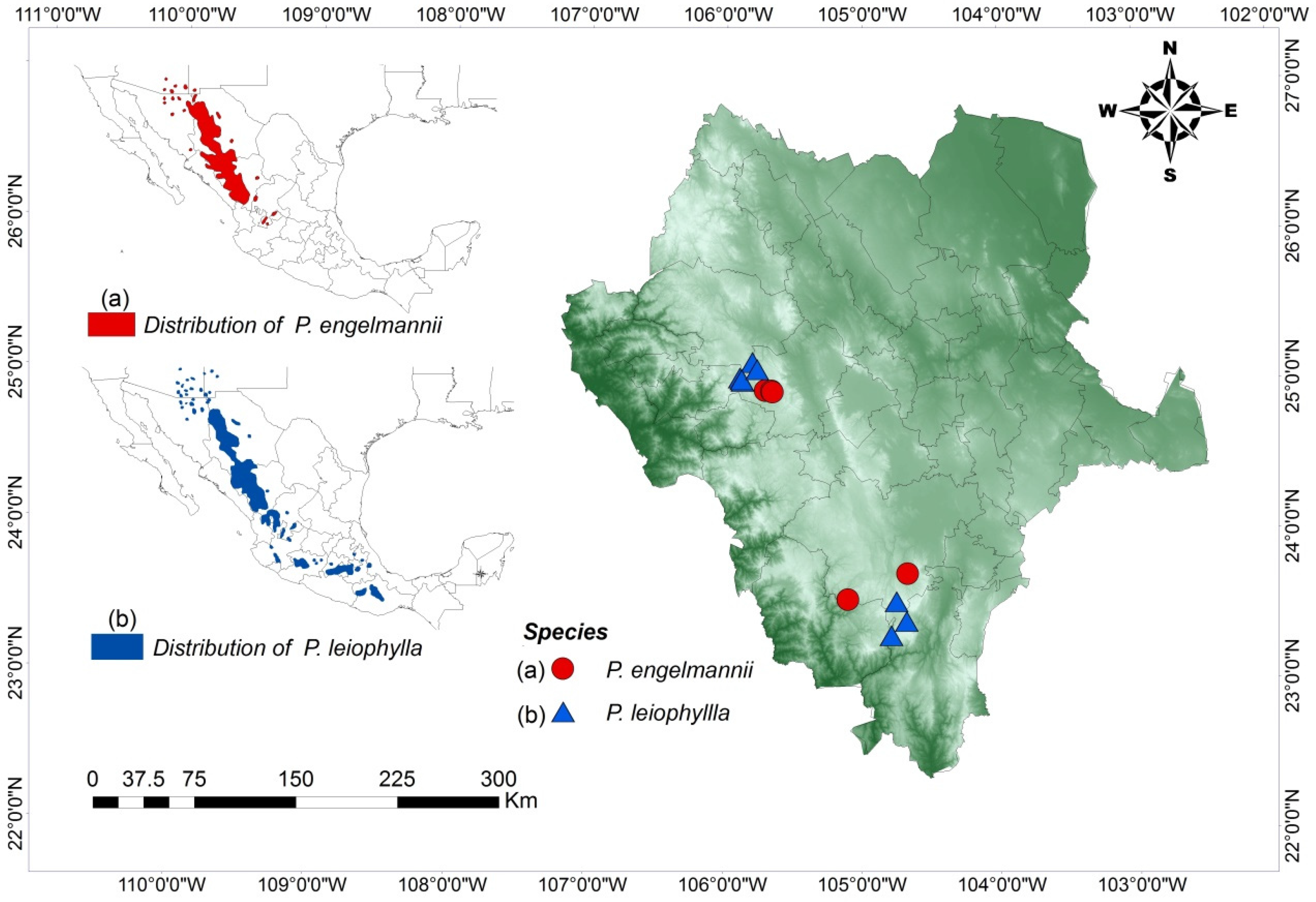
2.1. Study Area

Seven Apache pine (Pinus engelmannii (PE)) and nine Chihuahua pine (P. leiophylla var. leiophylla (PL)) seed stands in the Sierra Madre Occidental, Durango, Mexico were examined, as shown in Figure 1 and Table 1.
Each seed stand consisted of 130 adult trees that looked clearly superior in their dimension, quality, and disease resistance compared to the mean tree in each stand (for selection criteria, see Wehenkel et al. [23]. The size of the seed stands varied between 4.35 and 33.85 ha depending on the tree density. The stands were situated in natural populations mixed with other pine species (P. teocote, P. arizonica, and P. cooperi) as well as oak (Quercus sideroxyla), Juniper (Juniperus flacciada, J. deppeana), and Arbutus spp. For analysis of the SGS, samples of needles were randomly collected from 23–35 trees (from 130 trees) in each seed stand in 2013 (a total of 238 needle samples from PE and 298 from PL) (see more in Hernández-Velasco et al. [14]; Table 1).

2.2. Genetic Analysis

AFLP analysis of the sampled needles was performed according to Vos et al. [30]. As the genome of conifers is huge, the protocol was modified to include a greater number of adapters (restriction/ligature, 6 times) and primers (pre-AFLP and selective AFLP, 6 times). DNA was extracted using the QIAGEN DNeasy96 plant kit and digested with the restriction enzymes EcoRI (5′-GACTGCGTACCAATTCNNN-3′) and MseI (5′-GATGAGTCCTGAGTAANNN-3′). Polymerase Chain Reaction (PCR) amplification was then performed with double-stranded EcoRI and MseI adaptors ligated to the end of the restriction fragments, to produce template DNA. In pre-AFLP amplification, the PCR products were treated with the primer combination E01/M03 (EcoRI-A/MseI-G). Selective amplification was carried out with the fluorescent-labelled (FAM) primer pair E35 (EcoRI-ACA-3) and M63+C (MseI-GAAC) for PE and PL. The fourth selective base was added to reduce the large number of weak signals. The amplified restriction products were electrophoretically separated in a Genetic Analyzer (ABI 3100 16 capillaries, Foster City, CA, USA), along with the internal size standard GeneScan 500 ROX (fluorescent dye, obtained from Applied Biosystems, Foster City, CA, USA). The size of the AFLP fragments was resolved with the GeneScan 3.7 and Genotyper 3.7 software packages (Applied Biosystems, Foster City, CA, USA) (see details in Ávila-Flores et al. [31]).
Two binary AFLP matrices (one per species) were produced from the presence (code 1) or absence (code 0) at potential band positions. The appearance of a band indicates a dominant genetic variant (the “plus phenotype”) and the absence of a band indicates the recessive genetic (allelic) variants at the given position (locus) (the “minus phenotype”) [32,33]. Only AFLP matrices with frequencies of genetic variants above 0.05 and below 0.95 were included in further analyses.

2.3. Spatial Structural Analysis of AFLP Data

The geographical (spatial) distance was determined from the Euclidean distance between individuals, separately for each of the two tree species analyzed. The SGS within and among the seed stands was determined by analyzing three different coefficients of genetic distances. Tanimoto distance (TD) [34], Genetic Distance of Huff (GD) [35], and pairwise kinship coefficients (Fij) [9] were all considered because different mathematical approaches can produce contrasting conclusions (see details below). The distances were computed using Spatial Genetic Software v1.0 (SILVOLAB Guyane INRA Station de Recherches Forestières, Campus agronomique, Kourou cedex, French Guiana) [5], SPAGeDi v1.4 (Laboratoire de Gènètique et Ecologie vegetales, Universitè Libre de Bruxelles, Bruxelles, Belgium) [1], and GenAlEx v6.501 (Evolution, Ecology and Genetics, Research School of Biology, The Australian National University, Canberra, Australia and Department of Ecology, Evolution and Natural Resources, School of Environmental and Biological Sciences, Rutgers University, New Brunswick, NJ, USA) [14,36].
The “width” dimension of spatial distance classes was defined as including a minimum of 30 pairwise comparisons per distance class [37]. As the smallest width of the distance class could not be less than 150 m, all SGS statistics within the 16 seed stands were therefore calculated for the 150 m distance-class distributions.
For each spatial distance class, the observed values of the genetic distances were compared with the random value obtained using 999 permutations (in the case of Spatial Genetic Software, and SPAGeDi) or 999 bootstraps (using GenAlEx). To test whether SGS was significantly different from zero, a 99% confidence interval was then calculated for each genetic distance [5,38]. For each spatial distance class, the probability value (P) was also computed for each genetic distance. Bonferroni correction [39] was also performed to reduce the risk of obtaining false-positive results (type I errors). The corrected critical p value (significance level α* = 0.00036) was determined by dividing the original critical p value (0.025) by the number of comparisons or hypotheses (m = 69). Consequently, the Bonferroni critical value of P was 1 − α* = 0.9997 [14].
The genetic dissimilarity (Dij) between the binary vectors of two individuals, i and j, was calculated by using Spatial Genetic Software v1.0, as described for the TD [34]. Genetic distograms were then constructed to estimate the SGS. The overall mean value of the TD between all trees was used as a reference for random spatial structure [5].
The Fij for dominant markers in diploids was calculated to measure the occurrence of identical alleles at a given locus in a pair of individuals [9] by using SPAGeDi software ver.1.4 [40,41]. The Fij based on genetic markers actually estimates relative kinships that can be defined as ratios of the differences of impossible identities [42]. To detect the SGS, the Fij values were averaged over a group of distance classes and plotted against the Euclidean spatial distance. Positive values of Fij can be obtained for some individuals that are more closely related than random individuals, but negative Fij values occur if the individuals are less closely related than random individuals [9].
An individual-by-individual pairwise GD matrix (N × N) was created using GenAlEx v6.501. In regard to the GD, a comparison where individuals show the same state according to the AFLP (e.g., 0 vs. 0 and 1 vs. 1 comparison) yields a value of 0, while any comparison of different states (e.g., 0 vs. 1 and 1 vs. 0) yields a value of 1 [36]. An autocorrelation coefficient (r) was then computed using the matrices including pairwise geographic (Euclidean) distances and pairwise GD, which yielded the genetic distance between pairs of individuals within a defined distance class [36].

2.4. Kruskal Wallis Test

The Kruskal Wallis post-hoc test (Tukey and Kramer approach) [43,44] was used to check whether the observed differences in the values of the TD, GD, and Fij between each PE and PL stand occur as random events, rather than being caused by directed forces (significance level α = 0.05). The test was implemented using the R 3.2.2 statistical package (Foundation for Statistical Computing, Vienna, Austria) [45] and the PMCMR package (Federal Institute of Hydrology, Koblenz, Rhineland-Palatinate, Germany) [46].

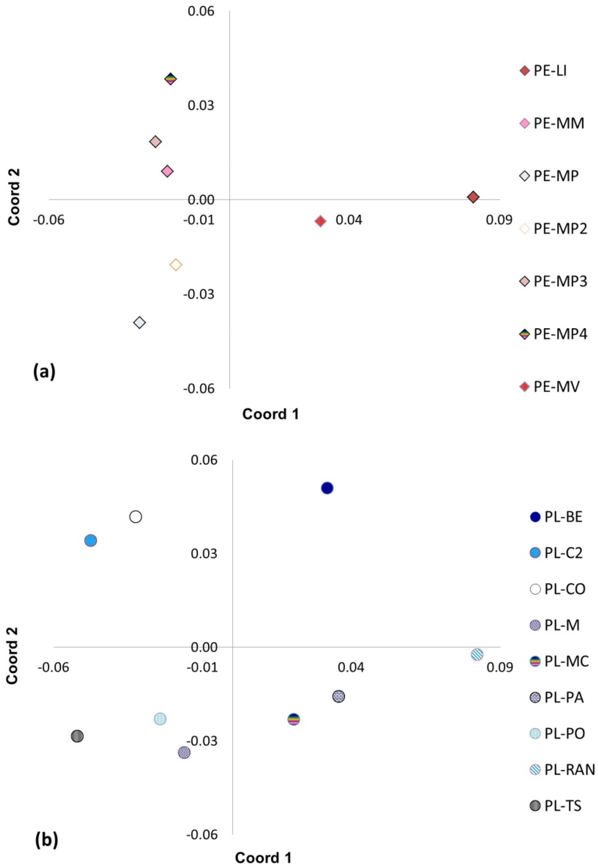
2.5. Principal Coordinate Analysis

The binary AFLP data matrix was also analyzed by Principal Coordinate Analysis (PCoA, Gresham College, London, UK), implemented with GenAlEx v6. Genetic differences between the seed stands and trees were calculated as Nei′s Genetic Distance (Brown University, Providence, RI, USA) [47,48]. The two first coordinates were used to represent genetic separation of populations and individuals.

3. Results

In total, all AFLP primer combinations tested in this study yielded 303 polymorphic bands of 77–450 bp across all Pinus engelmannii individuals and 325 polymorphic bands in the P. leiophylla individuals. Analysis of the SGS (using the Tanimoto distance) with 150 m distance-class distributions did not reveal any significant autocorrelation (after Bonferroni correction) within most of the P. engelmannii and P. leiophylla stands, except for the distance class of 300–450 m in the PL-CO stand (p ≥ 0.9997) (Table 2, Figure 2 and Figure 3). The mean genetic distance between P. engelmannii trees in the most southern population (Li stand) was significantly the smallest, whereas the significantly largest genetic distance in this study was found in the two most northern populations (MM and MP3 stands). However, the mean genetic differentiation (TD) between P. leiophylla trees was the smallest in a northern population (M stand), and the largest mean genetic differentiation observed in this study was found in another northern population (PO stand) (Table 2 and Table S1). On the other hand, statistically significant SGS was detected in almost all distance classes at large scale (among the seed stands) (Table 3 and Table 4, Tables S2 and S3, Figure 3 and Figure 4).
The results of the Kruskal-Wallis test showed that only the mean GD was statistically significantly larger in the P. leiophylla seed stands and not in the P. engelmannii seed stands (p = 0.013).
At the seed stand level, the PCA revealed clear separation between the stands for both species (Figure 5). The first three coordinates explained 85.93% (P. engelmannii) and 79.11% (P. leiophylla), respectively, of the variation found in the AFLP study. P. leiophylla stands were more genetically different than the P. engelmannii stands. By plotting the first two coordinates, which together describe 75.78% and 64.95%, respectively, of the AFLP variation, the P. engelmannii (PE) and the P. leiophylla (PL) populations were divided into three clusters, while the P. leiophylla (PL) stands were distributed in four clusters (Figure 5): (1) PE-MM, PE-MP, PE-MP2, PE-MP3, PE-MP4, (2) PE-MV and (3) PE-Li (Figure 5a); (1) PL-BE, (2) PL-RAN, (3) PL-PO, PL-PA, PL-TS, PL-MC, and PL-M, (3) and finally, (4) PL-C2, PL-CO were clearly genetically distinct from the other three clusters of P. leiophylla seed stands (Figure 5b).
In a PCoA conducted at the individual level, the first three coordinates explained a much lower percentage of the variation in the AFLP study (13.77% in P. engelmannii and 14.42% in P. leiophylla). Plotting the first two coordinates (which together explained 11.01% and 11.48%, respectively, of the variation in AFLP) showed that only P. engelmannii individuals were divided into separate groups (PE-Li vs. the rest of seed stands). P. leiophylla individuals per seed stand were genetically more dissimilar than the P. engelmannii individuals (Figure S1).

4. Discussion

As predicted, no significant SGS was detected within the 16 seed stands of the two tested pine species, Apache pine (P. engelmannii) and Chihuahua pine (P. leiophylla var. leiophylla) at the local level (Table 2 and Table S1). This matches several previous reports describing that no SGS could be observed in North American stands of conifer species such as Picea chihuahuana, Pseudotsuga menziesii, Pinus strobiformis [13], P. clausa [11], P. strobus [12], P. lumholtzii [6], P. cembroides, P. discolor, P. durangensis, and P. teocote [14]. According to Parker et al. [11] and Vekemans and Hardy [1], the main reason for the lack of significant SGS observed in these two pine species at the local level was probably the wind-mediated dispersal mating system, which leads to a strong omnidirectional gene flow.
However, there are other causes of random spatial distribution of genetic variants: (i) seed shadows of neighboring adult trees sometimes overlap; (ii) germination of seeds from numerous neighboring adult trees within relatively small stand patches; (iii) demographic mortality, which may also reduce the genetic relatedness at the seedling and sapling stages [6,11,49,50,51]; (iv) the disguising of SGS by high densities of adult trees; and (v) alteration of the tree stands by human intervention [14,50,52,53].
Among the P. engelmannii and P. leiophylla seed stands under study, and for almost all distance classes considered, the genetic and geographical distances between individual trees were significantly related (Table 3 and Table 4, Figure 2a and Figure 3, Tables S2 and S3). This confirms the theory of isolation by distance (i.e., limited dispersal caused by geographic distance) [54]. The limited dispersal mainly facilitates the genetic divergence of populations through drift and local adaptation. On the other hand, in the medium or long term restricted dispersal of pollen and seed can limit the genetic exchange between populations by reproductive segregation in the form of phenological isolation or ecological specialization [55].

5. Conclusions

Our findings have some important practical implications for future pine seed stand identification and management that can help avoid reforestation failure or inefficiencies, since non-local genotypes often are considered to have a fitness disadvantage over local genotypes [29]. First, the genetic variants were randomly mixed within the seed stands and were detected by non-significant genetic differences between the individual trees. In these stands, the maximum geographical distance between the studied trees was 600–1200 m (Table 2 and Table 3). Thus, the collection of seed in only some parts of these seed stands should not significantly alter the degree of genetic differentiation within the (collected) seed. Second, analysis of the seed stands showed that genetic differences between individuals at geographical distances of seven to eight kilometers for P. leiophylla and up to 24 km for P. engelmannii were significantly smaller than random genetic differences (Table 3 and Table 4, Tables S2 and S3), i.e., there was probably still sufficient genetic exchange between the trees at up to 8 km for P. leiophylla and up to 24 km for P. engelmannii. Thus, future seed orchards within these geographic distances may be exposed to external pollen contamination from other stands from the same tree species, which can decrease the genetic gain of a seed orchard crop (a contamination level of about 50% reduces the genetic gain by about 25%) [56].
The genetic exchange detected at larger scales is supported by Varis et al. [57] who reported a dispersal distance up to 600 km for P. sylvestris, and by Williams [58], who indicated a dispersal distance up to 40 km for P. taeda; although these findings were probably due to stepping stone events and not to single long distance results. Moreover, Robledo-Arnuncio [59] observed a significant level of effective pollen flow (up to 4.4%) from a large population located at a distance of 100 km. Moreover, the problem of pollen contamination in pine seed orchards due to insufficient distances from other stands was observed in various studies. For example, the estimated level of pollen contamination in Scot’s pine seed orchards varied between 2% and 74% [60]. Similar pine species could contaminate the seed orchards by hybridization within these distances, which seems to be common in P. engelmannii [31].
However, the seed stands under study here were already significantly genetically different in the distance classes of 24–48 km of P. engelmannii and 7–14 km of P. leiophylla (Table 3 and Table 4). Thus, distances between seed orchards and pollen propagators of more than 24 km for P. engelmannii and more than 7 km for P. leiophylla may be sufficient to limit the contamination. Finally, the significant differences in genetic structures lead us to conclude the following: (i) local seeds should be used for (re)forestation because they may also be locally adapted [61]; and (ii) a fine-scale network of forest seed stands is appropriate for conserving the different genetic structures [14].

Supplementary Materials

The following are available online at www.mdpi.com/1999-4907/8/1/22/s1, Figure S1: Results of Principal Coordinates Analysis (PCoA) of the individual Pinus engelmannii (a) and Pinus leiophylla trees (b). The first two coordinates together explained 11.01% and 11.48%, respectively, of the variation in AFLP. For definitions of the stand codes, see in caption of Figure 5 in the paper, Table S1: Analysis of fine-scale with GenAlex and SPAGeDi in seven seed stands of Pinus engelmannii and nine seed stands of P. leiophilla by considering a distance class width of 150 m, 999 bootstraps or 999 permutations and a 99% confidence interval. The genetic distance of Huff (GD) was calculated using GenAlEx 6.501. The pairwise kinship coefficient (Fij) was calculated using SPAGeDi 1.4, Table S2: Analysis of spatial genetic structure among seven Pinus engelmannii seed stands by considering a distance class width of 160 m in the northern stands and 24 km in the southern stands, 999 bootstraps and permutations and a 99% confidence interval. The genetic distance of Huff (GD) was calculated using GenAlEx 6.501, and the pairwise kinship coefficient (Fij) was calculated using SPAGeDi 1.4, Table S3: Analysis of large-scale spatial genetic structure in nine seed stands of Pinus leiophylla by considering a distance class width of 8 km in the stands, 999 bootstraps or 999 permutations and a 99% confidence interval. The genetic distance of Huff (GD) was calculated using GenAlEx 6.501, and the pairwise kinship coefficient (Fij) was calculated using SPAGeDi 1.4.

Acknowledgments

We thank the Unión de Permisionarios de la Unidad de Administración Forestal Santiago Papasquiaro S.C. and Permisionarios de la Unidad de Administración Forestal La Flor Durango A.C. (led by Fernando Salazar Jiménez and Julián Bautista Díaz, respectively), for their helpful assistance and the allocation of the data set.

Author Contributions

María Elena Ortiz-Olivas carried out the field data compilation and analysis, designed the Tables and Figures and wrote substantial text parts. José Ciro Hernández-Díaz, Matthias Fladung, Álvaro Cañadas-López and José Ángel Prieto-Ruíz reviewed drafts of the paper. Christian Wehenkel conceived the work, designed the experiments, carried out the field work, did the main writing and the coordination.

Conflicts of Interest

The authors declare no conflict of interest.

References

  1. Vekemans, X.; Hardy, O.J. New insights from fine-scale spatial genetic structure analyses in plant populations. Mol. Ecol. 2004, 13, 921–935. [Google Scholar] [CrossRef] [PubMed]
  2. Van Rossum, F.; Triest, L. Fine-Scale genetic structure of the common Primula elatior (Primulaceae) at an early stage of population fragmentation. Am. J. Bot. 2006, 93, 1281–1288. [Google Scholar] [CrossRef] [PubMed]
  3. Ledoux, J.B.; Garrabou, J.; Bianchimani, O.; Drap, P.; FÉRAL, J.P.; Aurelle, D. Fine-Scale genetic structure and inferences on population biology in the threatened Mediterranean red coral, Corallium rubrum. Mol. Ecol. 2010, 19, 4204–4216. [Google Scholar] [CrossRef] [PubMed]
  4. Segelbacher, G.; Cushman, S.A.; Epperson, B.K.; Fortin, M.J.; Francois, O.; Hardy, O.J.; Holderegger, R.; Taberlet, P.; Waits, L.P.; Manel, S. Applications of landscape genetics in conservation biology: Concepts and challenges. Conserv. Genet. 2010, 11, 375–385. [Google Scholar] [CrossRef]
  5. Degen, B.; Petit, R.; Kremer, A. SGS—Spatial Genetic Software: A Computer Program for Analysis of Spatial Genetic and Phenotypic Structures of Individuals and Populations. J. Hered. 2001, 92, 447–449. [Google Scholar] [CrossRef] [PubMed]
  6. Reyes-Murillo, C.A.; Hernández-Díaz, J.C.; Heinze, B.; Prieto-Ruiz, J.Á.; López-Sánchez, C.A.; Wehenkel, C. Spatial genetic structure in seed stands of Pinus lumholtzii BL Rob. & Fernald in Durango, Mexico. Tree Genet. Genomes 2016, 12, 1–10. [Google Scholar]
  7. Mueller, U.G.; Wolfenbarger, L.L. AFLP genotyping and fingerprinting. Trends Ecol. Evol. 1999, 14, 389–394. [Google Scholar] [CrossRef]
  8. Hardy, I.C.W.; Goubault, M.; Batchelor, T.P. Hymenopteran contests and agonistic behaviour. In Animal Contests; Hardy, I.C.W., Briffa, M., Eds.; Cambridge University Press: Cambridge, UK, 2013; pp. 147–177. [Google Scholar]
  9. Hardy, O.J. Estimation of pairwise relatedness between individuals and characterization of isolation-by-distance processes using dominant genetic markers. Mol. Ecol. 2003, 12, 1577–1588. [Google Scholar] [CrossRef] [PubMed]
  10. Krauss, S.L.; Sinclair, E.A.; Bussell, J.D.; Hobbs, R.J. An ecological genetic delineation of local seed-source provenance for ecological restoration. Ecol. Evol. 2013, 3, 2138–2149. [Google Scholar] [CrossRef] [PubMed]
  11. Parker, K.C.; Hamrick, J.L.; Parker, A.J.; Nason, J.D. Fine-Scale genetic structure in Pinus clausa (Pinaceae) populations: Effects of disturbance history. Heredity 2001, 87, 99–113. [Google Scholar] [CrossRef] [PubMed]
  12. Epperson, B.K.; Gi Chung, M. Spatial genetic structure of allozyme polymorphisms within populations of Pinus strobus (Pinaceae). Am. J. Bot. 2001, 88, 1006–1010. [Google Scholar] [CrossRef] [PubMed]
  13. Quiñones-Pérez, C.Z.; Simental-Rodríguez, S.L.; Sáenz-Romero, C.; Jaramillo-Correa, J.P.; Wehenkel, C. Spatial genetic structure in the very rare and species-rich Picea chihuahuana tree community (Mexico). Silvae. Genet. 2014, 63, 149–159. [Google Scholar]
  14. Hernández-Velasco, J.; Hernández-Díaz, J.C.; Fladung, M.; Cañadas-López, A.; Prieto-Ruíz, J.A.; Wehenkel, C. Spatial genetic structure in four Pinus species in the Sierra Madre Occidental, Durango, México. Can. J. For. Res. 2016. [Google Scholar] [CrossRef]
  15. Rzedowski, J.; Huerta, L. Vegetación de México. Available online: http://www.biodiversidad.gob.mx/publicaciones/librosDig/pdf/VegetacionMxPort.pdf (accessed on 6 January 2017).
  16. Comisión Nacional Forestal (CONAFOR). Inventario Nacional Forestal y de Suelos de México 2004–2009, 1st ed.; CONAFOR: Zapopan, Mexico, 2009; p. 206. [Google Scholar]
  17. Rodríguez-Banderas, A.; Vargas-Mendoza, C.F.; Buonamici, A.; Vendramin, G.G. Genetic diversity and phylogeographic analysis of Pinus leiophylla: A post-glacial range expansion. J. Biogeogr. 2009, 36, 1807–1820. [Google Scholar] [CrossRef]
  18. Ávila-Flores, I.J.; Hernández-Díaz, J.C.; González-Elizondo, M.S.; Prieto-Ruíz, J.A.; Wehenkel, C. Pinus engelmannii Carr. In Northwestern Mexico: A Review. Pak. J. Bot. 2016, 5. in press. [Google Scholar]
  19. González Elizondo, M.S.; González Elizondo, M.; Márquez Linares, M.A. Vegetación y Ecorregiones de Durango; Plaza y Valdés Editores-Instituto Politécnico Nacional: Distrito Federal, Mexico, 2007; p. 220. [Google Scholar]
  20. González-Elizondo, M.S.; González-Elizondo, M.; Ruacho-González, L.; López-Enríquez, L.; Retana-Rentería, F.I.; Tena-Flores, J.A. Ecosystems and Diversity of the Sierra Madre Occidental. Available online: https://www.fs.fed.us/rm/pubs/rmrs_p067/rmrs_p067_204_211.pdf (accessed on 6 January 2017).
  21. Silva-Flores, R.; Pérez-Verdín, G.; Wehenkel, C. Patterns of tree species diversity in relation to climatic factors on the Sierra Madre Occidental, Mexico. PLoS ONE 2014, 9, e105034. [Google Scholar] [CrossRef] [PubMed]
  22. Wehenkel, C.; Corral-Rivas, J.J.; Hernández-Díaz, J.C.; von Gadow, K. Estimating balanced structure areas in multi-species forests on the Sierra Madre Occidental, Mexico. Ann. For. Sci. 2011, 68, 385–394. [Google Scholar] [CrossRef]
  23. Wehenkel, C.; Simental-Rodríguez, S.L.; Silva-Flores, R.; Hernández-Díaz, J.C.; López-Sánchez, C.A.; Antúnez, P. Discrimination of 59 seed stands of various Mexican pine species based on 43 dendrometric, climatic, edaphic and genetic traits. Forstarchiv 2015, 86, 194–201. [Google Scholar]
  24. Farjon, A. Pinus engelmannii. The IUCN Red List of Threatened Species. Available online: http://www.iucnredlist.org/details/42362/0 (accessed on 14 June 2016).
  25. Farjon, A. Pinus leiophylla. The IUCN Red List of Threatened Species. Available online: http://www.iucnredlist.org/details/42376/0 (accessed on 22 July 2016).
  26. Mejía-Bojorquez, J.M.; Prieto-Ruíz, J.Á.; García-Cuevas, X.; García-Rodríguez, J.L.; Muñoz-Flores, H.J; Rosales-Mata, S. Evaluación de plantaciones comerciales en el Estado de Durango. In Evaluación de reforestaciones en la Sierra Madre Occidental; Muñoz-Flores, H.J., Prieto-Ruíz, J.A., Ruedas-Sánchez, A., Alarcón-Bustamante, M., Eds.; Campo experimental Valle del Guadiana, CIRNOC.INIFAP: Durango, Mexico, 2011; pp. 57–86. [Google Scholar]
  27. Castelán-Muñoz, N. Fisiología de Plántulas de Pinus Leiophylla Sometidas a Estrés Hídrico. Master’s Thesis, Colegio de Postgraduados, Texcoco, Mexico, 2014. [Google Scholar]
  28. Wehenkel, C.; Cruz-Cobos, F.; Carrillo, A.; Lujan-Soto, J.E. Estimating bark volumes for 16 native tree species on the Sierra Madre Occidental, Mexico. Scand. J. For. Res. 2012, 27, 578–585. [Google Scholar] [CrossRef]
  29. Slavov, G.T.; Howe, G.T.; Adams, W.T. Pollen contamination and mating patterns in a Douglas-fir seed orchard as measured by simple sequence repeat markers. Can. J. For. Res. 2005, 35, 1592–1603. [Google Scholar] [CrossRef]
  30. Vos, P.; Hogers, R.; Bleeker, M.; Reijans, M.; Van Lee, T.; Hornes, M.; Frijters, A.; Pot, J.; Zabeau, M. AFLP: A new technique for DNA fingerprinting. Nucleic Acids Res. 1995, 23, 4407–4414. [Google Scholar] [CrossRef] [PubMed]
  31. Ávila-Flores, I.J.; Hernández-Díaz, J.C.; González-Elizondo, M.S.; Prieto-Ruíz, J.A.; Wehenkel, C. Spatial genetic structure and degree of hybridization in seed stands of Pinus engelmannii Carr. in the Sierra Madre Occidental, Durango, Mexico. PLoS ONE 2015, 11, e0152651. [Google Scholar]
  32. Krauss, S.L. Accurate gene diversity estimates from amplified fragment length polymorphism (AFLP) markers. Mol. Ecol. 2000, 9, 1241–1245. [Google Scholar] [CrossRef] [PubMed]
  33. Bonin, A.; Bellemain, E.; Bronken, E.P.; Pompanon, F. How to track and assess genotyping errors in population genetics studies. Mol. Ecol. 2004, 13, 3261–3273. [Google Scholar] [CrossRef] [PubMed]
  34. Deichsel, G.; Trampisch, H.J. Cluster Analyse und Diskriminanz Analyse; Gustav Fischer Verlag: Stuttgart, Germany, 1985; p. 880. [Google Scholar]
  35. Huff, D.R.; Peakall, R.; Smouse, P.E. RAPD variation within and among natural populations of outcrossing buffalo grass Buchloe dactyloides (Nutt) Engelm. Theor. Appl. Genet. 1993, 86, 927–934. [Google Scholar] [CrossRef] [PubMed]
  36. Peakall, R.; Smouse, P.E. GenAlEx 6.5: Genetic analysis in Excel. Population genetic software for teaching and research-an update. Bioinformatics 2012, 28, 2537–2539. [Google Scholar] [CrossRef] [PubMed]
  37. Doligez, A.; Joly, H.I. Genetic diversity and spatial structure within a natural stand of a tropical forest tree species, Carapa procera (Meliaceae), in French Guiana. Heredity 1997, 79, 72–82. [Google Scholar] [CrossRef]
  38. Manly, B.F. Randomization Bootstrap and Monte Carlo Methods in Biology, 3rd ed.; Chapman and Hall/CRC: London, UK, 1997; p. 480. [Google Scholar]
  39. Hochberg, Y. A sharper Bonferroni procedure for multiple tests of significance. Biometrika 1988, 75, 800–802. [Google Scholar] [CrossRef]
  40. Hardy, O.J.; Vekemans, X. SPAGeDi: A versatile computer program to analyse spatial genetic structure at the individual or population levels. Mol. Ecol. Notes 2002, 2, 618–620. [Google Scholar] [CrossRef]
  41. SPAGeDi software ver. 1.4. 2016. Available online: http://ebe.ulb.ac.be/ebe/Software.html (accessed on 10 August 2016).
  42. Rousset, F. Inbreeding and relatedness coefficients: What do they measure? Heredity 2002, 88, 371–380. [Google Scholar] [CrossRef] [PubMed]
  43. Kruskal, W.H.; Wallis, W.A. Use of Ranks in One-Criterion Variance Analysis. J. Am. Stat. Assoc. 1952, 47, 583–621. [Google Scholar] [CrossRef]
  44. Sachs, L. Angewandte Statistik; Springer: Belin, Germany, 1997; p. 155. [Google Scholar]
  45. R Core Team. R: A Language and Environment for Statistical Computing; R Foundation for Statistical Computing: Vienna, Austria, 2013. [Google Scholar]
  46. Pohlert, T. The Pairwise Multiple Comparison of Mean Ranks Package (PMCMR). 2014. Available online: https://cran.r-project.org/web/packages/PMCMR/vignettes/PMCMR.pdf (accessed on 11 February 2014).
  47. Nei, M. Genetic distance between populations. Amer. Nat. 1972, 106, 283–392. [Google Scholar] [CrossRef]
  48. Nei, M. Estimation of average heterozygosity and genetic distance from a small number of individuals. Genetics 1978, 89, 583–590. [Google Scholar] [PubMed]
  49. Epperson, B.K.; Alvarez-Buylla, E.R. Limited seed dispersal and genetic structure in life stages of Cecropia obtusifolia. Evolution 1997, 51, 275–282. [Google Scholar] [CrossRef]
  50. Hamrick, J.L.; Murawski, D.A.; Nason, J.D. The influence of seed dispersal mechanisms on the genetic structure of tropical tree populations. Vegetatio 1993, 107–108, 281–297. [Google Scholar]
  51. Fuchs, E.J.; Hamrick, J.L. Spatial genetic structure within size classes of the endangered tropical tree Guaiacum sanctum (Zygophyllaceae). Am. J. Bot. 2010, 97, 1200–1207. [Google Scholar] [CrossRef] [PubMed]
  52. Hamrick, J.L.; Nason, J.D. Consequences of dispersal in plants. In Population Dynamics in Ecological Space and Time; Rhodess, O.E., Jr., Chesser, R.K., Smith, M.H., Eds.; University of Chicago Press: Chicago, IL, USA, 1996; pp. 203–236. [Google Scholar]
  53. Jordano, P.; Garcia, C.; Godoy, J.A.; Garcia-Castano, J.L. Differential contribution of frugivores to complex seed dispersal patterns. Proc. Natl. Acad. Sci. USA 2007, 104, 3278–3288. [Google Scholar] [CrossRef] [PubMed]
  54. Wright, S. Isolation by distance. Genetics 1943, 28, 114–138. [Google Scholar] [PubMed]
  55. Peterson, M.A.; Denno, R.F. The influence of dispersal and diet breadth on patterns of genetic isolation by distance in phytophagous insects. Amer. Nat. 1998, 152, 428–446. [Google Scholar] [CrossRef] [PubMed]
  56. Prescher, F. Seed Orchards–Genetic Considerations on Function, Management and Seed Procurement. Ph.D. Thesis, Swedish University of Agricultural Sciences, Uppsala, Sweden, 2007. [Google Scholar]
  57. Varis, S.; Pakkanen, A.; Galofré, A.; Pulkkinen, P. The extent of south-north pollen transfer in Finnish Scots pine. Silva Fenn. 2009, 43, 717–726. [Google Scholar] [CrossRef]
  58. Williams, C.G. Long-Distance pine pollen still germinates after meso-scale dispersal. Am. J. Bot. 2010, 97, 846–855. [Google Scholar] [CrossRef] [PubMed]
  59. Robledo-Arnuncio, J.J. Wind pollination over mesoscale distances: An investigation with Scots pine. New Phytol. 2011, 190, 222–233. [Google Scholar] [CrossRef] [PubMed]
  60. Ivanek, O.; Procházková, Z.; Matĕjka, K. Analysis of the genetic structure of a model Scots pine (Pinus sylvestris) seed orchard for development of management strategies. J. For. Sci. 2013, 59, 377–385. [Google Scholar]
  61. Vander Mijnsbrugge, K.; Bischoff, A.; Smith, B. A question of origin: Where and how to collect seed for ecological restoration. Basic Appl. Ecol. 2010, 11, 300–311. [Google Scholar] [CrossRef]
Figure 1. Locations of the Pinus engelmannii and P. leiophylla 16 seed stands in the Sierra Madre Occidental, Durango, Mexico. Maps showing the distribution areas of P. engelmannii and P. leiophylla (a) and the locations of the seven P. engelmannii and nine P. leiophylla seed stands under study in the Sierra Madre Occidental, Durango, Mexico (b). Seed stands: La Lisuda (PE-Li), Mesa de Mingarreta (PE-MM), Mesa de Perdederos 1 (PE-MP), Mesa de Perdederos 2 (PE-MP2), Mesa de Perdederos 3 (PE-MP3), Mesa de Perdederos 4 (PE-MP4), La Mesa de Veracruz (PE-MV), Bajío (PL-BE), Coloradas (PL-C2), Cócono (PL-CO), Maguey (PL-M), Mesa de Cristo (PL-MC), Patio (PL-PA), Polvorín (PL-PO), Rancho (PL-RAN), and Tijera de Salsipuedes (PL-TS).
Forests 08 00022 g001
Figure 2. Analysis of fine-scale spatial genetic structure of two seed stands. Analysis of fine-scale spatial genetic structure of the seed stands (a) La Mesa de Veracruz (Pinus engelmannii) and (b) Cócono (P. leiophylla) by considering a distance class of size 150 m. Distogram calculated using the mean Tanimoto distance (TD). CI = confidence interval.
Forests 08 00022 g002
Figure 3. Analysis of large-scale spatial genetic structure in Pinus engelmannii. Analysis of large-scale spatial genetic structure in seven seed stands of P. engelmannii by considering a distance class of size 160 m in the north, and 24 km in the south. Distogram calculated using the mean Tanimoto distance (TD). CI = confidence interval, (a) northern stands; (b) southern stands.
Forests 08 00022 g003
Figure 4. Analysis of large-scale spatial genetic structure in nine seed stands of P. leiophylla considering a distance class of size 8 km. Distogram calculated using the mean Tanimoto distance (TD), CI = confidence interval, (a) northern stands; (b) southern stands.
Forests 08 00022 g004
Figure 5. Results of Principal Coordinate Analysis (PCoA) at the stand level, with AFLP (amplified fragment length polymorphisms). For Pinus engelmannii (a) and Pinus leiophylla (b) the first two coordinates of PCoA together explained 75.78% and 64.95%, respectively, of the variation. Seed stands: La Lisuda (PE-Li), Mesa de Mingarreta (PE-MM), Mesa de Perdederos 1 (PE-MP), Mesa de Perdederos 2 (PE-MP2), Mesa de Perdederos 3 (PE-MP3), Mesa de Perdederos 4 (PE-MP4), La Mesa de Veracruz (PE-MV), Bajío (PL-BE), Coloradas (PL-C2), Cócono (PL-CO), Maguey (PL-M), Mesa de Cristo (PL-MC), Patio (PL-PA), Polvorín (PL-PO), Rancho (PL-RAN), and Tijera de Salsipuedes (PL-TS).
Forests 08 00022 g005
Table 1. Location, and some characteristics (sample size (N), elevation (E), mean distance between the trees (MD), Clark and Evans (1954) aggregation index (CE)) of the seven seed stands of Pinus engelmannii and nine seed stands of P. leiophylla under study in the Sierra Madre Occidental, Durango, Mexico.
CodeSPNLocationMunicipalityLatitude (North)Longitude (West)E (m)MD (m)CE
PE-LiPE35La LisudaPueblo Nuevo23°32′11″105°06′00″252335.561.070
PE-MMPE35Mesa de MingarretaSantiago Papasquiaro24°55′48″105°42′25″241855.151.121
PE-MPPE35Mesa de Perdederos 1Santiago Papasquiaro24°55′15″105°39′36″242057.780.984
PE-MP2PE35Mesa de Perdederos 2Santiago Papasquiaro24°55′27″105°39′41″244352.221.201
PE-MP3PE34Mesa de Perdederos 3Santiago Papasquiaro24°55′36″105°39′38″242461.481.354
PE-MP4PE35Mesa de Perdederos 4Santiago Papasquiaro24°55′08″105°39′15″242453.740.98
PE-MVPE35La Mesa de VeracruzDurango23°42′34″104°40′04″239066.491.257
PL-BEPL23BajíoMezquital23°23′27″104°40′27″255164.091.225
PL-C2PL35ColoradasMezquital23°17′49″104°47′08″245141.580.970
PL-COPL34CóconoDurango23°31′28″104°44′51″274240.070.969
PL-MPL35MagueySantiago Papasquiaro25°07′05″105°48′06″251847.50.873
PL-MCPL34Mesa de CristoSantiago Papasquiaro24°59′29″105°52′24″257538.270.916
PL-PAPL35PatioSantiago Papasquiaro25°00′48″105°53′38″250030.360.689
PL-POPL33PolvorínSantiago Papasquiaro25°00′05″105°52′47″250831.180.940
PL-RANPL35RanchoSantiago Papasquiaro25°00′05″105°52′47″247526.151.034
PL-TSPL34Tijera de SalsipuedesSantiago Papasquiaro25°04′17″105°46′05″254199.860.872
Note: SP = tree species.
Table 2. Analysis of fine-scale spatial genetic structure in seven seed stands of Pinus engelmannii and nine seed stands of P. leiophylla using a distance class width of 150 m, 999 permutations, and a 99% confidence interval. The Tanimoto distance (TD) was calculated using Spatial Genetic Software 1.0 [5].
Spatial Genetic Software
CodeNMDTDP(TD) < (−CI)P(TD) > (+CI)MT
PE-LI3535.560.45330.857 (150–300)0.965 (300–450)49 (600–750)
PE-MM3457.780.51190.727 (0–150)0.681 (300–450)38 (450–600)
PE-MP3555.150.50720.836 (600–750)0.753 (300–450)40 (600–750)
PE-MP23552.220.49280.772 (0–150)0.885 (450–600)48 (450–600)
PE-MP33561.480.50880.984 (150–300)0.968 (600–750)37 (600–750)
PE-MP43553.740.45940.950 (150–300)0.983 (450–600)63 (600–750)
PE-MV2970.770.49090.885 (0–150)0.813 (450–600)61 (600–750)
PL-BE2364.090.49460.837 (150–300)0.902 (300–450)41 (0–150)
PL-C23541.580.54990.911 (0–150)0.833 (300–450)64 (450–600)
PL-CO3440.070.51500.994 (150–300)0.9999 + (300–450)146 (0–150)
PL-M3547.50.48540.994 (0–150)0.941 (300–450)143 (0–150)
PL-MC3438.270.49560.988 (0–150)0.766 (150–300)40 (450–600)
PL-PA3530.360.49980.812 (150–300)0.973 (450–600)35 (600–750)
PL-PO3331.180.55950.986 (150–300)0.983 (0–150)43 (300–450)
PL-RAN3526.150.49280.856 (0–150)0.988 (300–450)85 (300–450)
PL-TS3499.860.53430.868 (1050–1200)0.914 (0–150)32 (0–150, 1050–1200)
Note: N = sample size; MD = mean distance to the next pine under study; TD = calculated average of the Tanimoto distance; MT = minimum tree pairs per class (distance class); CI = confidence interval; P(TD) < −CI and P(TD) > +CI, highest probability of autocorrelation in each stand, showing the distance class (m) where it was found; + indicates a significant difference after Bonferroni correction. For definitions of the stand codes, see in Table 1.
Table 3. Analysis of spatial genetic structure among P. engelmannii seed stands by considering a distance class width of 160 m in the northern stands and 24 km in the southern stands, 999 permutations, and a 99% confidence interval. The mean Tanimoto distance (TD) was calculated using Spatial Genetic Software 1.0 [5].
CodeNMDTDP(TD) < (−CI)P(TD) > (+CI)MTClasses
NORTH14055.680.50470.9999 (0–160) +0.9999 (320–480) +32 (0–160)10
0.9999 (160–320) +0.9999 (480–640) +
0.9999 (960–1120) +0.9999 (640–800) +
SOUTH6451.510.48370.9999 (0–24) +0.9549 (24–48)997 (24–48)2
Note: TD = mean Tanimoto distance; MT = minimum number of pairs per class (distance class), MD = mean distance to the next tree; CI = confidence interval; P(TD) < −CI and P(TD) > +CI, highest probability of autocorrelation in each stand, showing the distance class (m or km) where it was found; + indicates a significant difference after Bonferroni correction.
Table 4. Analysis of spatial genetic structure among seed stands of Pinus leiophylla by considering a distance class width of 8 km in the seed stands, 999 permutations, and a 99% confidence interval. The Tanimoto distance (TD) was calculated using Spatial Genetic Software 1.0 [5].
CodeNMDTDP(TD) < (−CI)P(TD) > (+CI)MTClasses
NORTH20645.470.54250.9999 (0–8) +0.9976 (24–32)2349 (28–35)4
0.9999 (16–24) +
SOUTH9246.650.54130.9999 (0–8) +0.9999 (8–16) +732 (8–16)3
Note: TD = mean Tanimoto distance; MT = minimum of pairs per class (distance class), MD = mean distance to the next tree; P = probability of autocorrelation; CI = confidence interval; + indicates a significant difference after Bonferroni correction.

