Acoustic-Based Non-Destructive Estimation of Wood Quality Attributes within Standing Red Pine Trees

Canadian Wood Fibre Centre, Canadian Forest Service, Natural Resources Canada, Sault Ste. Marie, P6A 2E5 ON, Canada
Forests 2017, 8(10), 380; https://doi.org/10.3390/f8100380
Submission received: 27 July 2017
/
Revised: 21 September 2017
/
Accepted: 30 September 2017
/
Published: 4 October 2017
(This article belongs to the Section Forest Inventory, Modeling and Remote Sensing)
Abstract
:The relationship between acoustic velocity (vd) and the dynamic modulus of elasticity (me), wood density (wd), microfibril angle, tracheid wall thickness (wt,), radial and tangential diameters, fibre coarseness (co) and specific surface area (sa), within standing red pine (Pinus resinosa Ait.) trees, was investigated. The data acquisition phase involved 3 basic steps: (1) random selection of 54 sample trees from 2 intensively-managed 80-year-old plantations in central Canada; (2) attainment of cardinal-based vd measurements transecting the breast-height position on each sample tree; and (3) felling, sectioning and obtaining cross-sectional samples from the first 5.3 m sawlog from which Silviscan-based area-weighted mean attribute estimates were determined. The data analysis phase consisted of applying graphical and correlation analyses to specify regression models for each of the 8 attribute-acoustic velocity relationships. Results indicated that viable relationships were obtained for me, wd, wt, co and sa based on a set of statistical measures: goodness-of-fit (42%, 14%, 45%, 27% and 43% of the variability explained, respectively), lack-of-fit (unbiasedness) and predictive precision (±12%, ±8%, ±7%, ±8% and ±6% error tolerance intervals, respectively). Non-destructive approaches for estimating the prerequisite wd value when deploying the analytical framework were also empirically evaluated. Collectively, the proposed approach and associated results provide the foundation for the development of a comprehensive and precise end-product segregation strategy for use in red pine management.
1. Introduction
The future prosperity of the Canadian forest sector is increasingly dependent on its ability to embrace value-based management given that the economic viability of the traditional volumetric yield maximization proposition is becoming more challenging. Principally, this is due to a combination of factors which include increasing global competiveness, accessibility of economically-viable fibre sources, and evolving market demands for increased end-product diversity and value (e.g., [1,2,3]). Operationally, this transitional shift has generated a renewed focus on deploying intensive silvicultural-based crop plans that can result in improvements in wood quality and the production of a more diverse stream of end-products throughout the rotation [4]. Such a representative crop plan would consist of species, genotype and initial spacing control via plantation establishment of genetically-improved stock on well-prepared (scarified) sites followed by early vegetation management treatments and subsequent maintenance of optimal site occupancy levels through density management treatments (e.g., precommercial and commercial thinning; [5]). Transitioning to a value-based management paradigm also requires improved operational intelligence for decision-making, particularly in relation to segregation and merchandising efficiency within the upstream portion of the forest products supply chain.
The quality and associated economic value of manufactured wood-based end-products derived from the merchantable stem portion of a harvested tree, such as pulp and paper products, dimensional lumber, engineered wood composites and utility poles, are largely dependent on the characteristics of internal fibre attributes (Table 1). The ability to estimate these internal attributes and by extension classify standing trees according to their end-product potential before harvest, could provide the prerequisite information for optimal segregation decision-making (e.g., directing the trees to the most appropriate conversion facility upon harvest (pole yards, pulp and paper mills or saw mills)).
Relatively recently, a suite of innovative non-destructive operational survey tools have been developed for estimating the end-product potential of standing trees. These tools include: (1) time-of-flight acoustic velocity instruments for indirectly providing an estimate of wood stiffness such as the Director ST300 developed by Fibre-gen Inc. of Christchurch, New Zealand (e.g., [8]) and the TreeSonic microsecond timer developed by Fakopp Enterprise, Ágfalva, Hungary (e.g., [9]); and (2) micro-drill resistance and impact tools for indirectly providing a non-destructive estimate of wood density such as the Resistograph developed by Instrumenta Mechanik Labor GmbH of Wiesloch, Germany, and the Pilodyn developed by PROCEQ of Zurich, Switzerland, respectively (see [10] for a comparative review).
Traditionally, one of the more important attributes associated with lumber quality and associated value as evident from its use in machine stress lumber grading [11], is the degree of bending stiffness as quantified by the static modulus of elasticity. This attribute has been historically determined through destructive, laborious and expensive bending stress tests of the extracted end-product (e.g., dimensional lumber). However, its dynamic analogue (dynamic modulus of elasticity) has been shown to be a useful surrogate measure of static wood stiffness that can be non-destructively determined through its relationship to acoustic velocity and wood density (e.g., [8,12,13]). The dynamic and static modulus of elasticity estimates have been shown to be highly correlated with each other (correlation coefficients >0.95) when compared within the same solid wood product (lumber), with the dynamic estimate being approximately 10% greater than that of the static value for a given wood sample (sensu [14]). Furthermore, based on comprehensive reviews, the acoustic-based approach has been shown to be of consequential utility in the non-destructive estimation of wood stiffness of both standing trees and harvested logs (e.g., [15]).
Conceptually, the velocity of a dilatational stress wave arising from a mechanically-induced impact that propagates through a standing tree, is related to dynamic modulus of elasticity according to Equation (1) (sensu [16,17]):
where me is the dynamic modulus of elasticity or MOEdyn (GPa), P is a species- or sample-specific transverse/axial stain ratio (Poisson ratio) estimate that is commonly treated as an unknown constant when parameterizing the relationship, wd(g) is a species- or sample-specific green wood density (kg/m3) estimate, and vd is the speed of the mechanically-induced dilatational stress wave (km/s) that propagates between a lower and upper probe positioned approximately at stem heights of 0.3 and 1.5 m, respectively. Deployments of simplified representations of this relationship in which acoustic velocity is singularly assumed to be an indirect measure of wood stiffness have been used as a surrogate response metric for evaluating thinning effects on wood quality (e.g., in Loblolly pine (Pinus taeda L.; [18]) and Douglas-fir (Pseudotsuga menziesii (Mirb.) Franco; [19]). In other simplified applications, a universal constant has been used in place of the species- or sample-specific wd(g) estimate (e.g., [8,20]).
Operationally, in-forest segregation decisions based on acoustic-based stiffness estimates may result in optimal wood allocations and accompanying increases in economic profitability [21]. However, empirical evaluations of the functional expression given by Equation (1) in which the dynamic modulus of elasticity and wood density are actually measured on clear xylem samples extracted from standing softwood trees, have shown considerable variation among investigations. Particularly, in terms of statistical significance, proportion of variability explained and precision of the resultant estimates (e.g., as reviewed by Hong ([8]) and Mora ([9])). Differences among studies in relation to species, locale, silvicultural treatment histories, instrumentation, environmental conditions at the time of sampling, and analytical approaches, have negated a definitive and conclusive determination of the overall merits of the acoustic approach to wood quality estimation. The degree of between-study variability suggests that acoustic relationships may be unique to the experimental approach and sample population utilized, and hence may be best evaluated on a species-, locale- and analytical- specific basis.
Advances in attribute determination via the introduction of the Silviscan system [22,23] have provided a means to evaluate the acoustic approach without resorting to costly and time-consuming methods. Briefly, the Silviscan system is an automated fibre analysis system originally developed by CSIRO’s (Commonwealth Scientific and Industrial Research Organisation) Forestry and Forest Products Division, in Australia. Based on a semi-empirical analytical approach, the system was designed to provide rapid and cost-effective estimates of wood quality attributes related to end-use performance [24]. Utilizing the Silviscan-based modulus of elasticity estimate and the oven-dry wood density estimate (wd) as a surrogate for wd(g), Hong ([8]) established a statistically significant (p ≤ 0.05) acoustic relationship for 778 standing Scot pine (Pinus sylvestris L.) trees growing in northern Sweden. In that study, 67% of the variation in the dynamic modulus of elasticity was explained by a simple linear regression model specification. Similarly, using Silviscan-based estimates of me and wd in conjunction with a simple linear regression model, Newton ([25]) established a statistically significant (p ≤ 0.05) acoustic relationship for 54 standing jack pine (Pinus banksiana Lamb.) trees growing in the central portion of the Canadian Boreal Forest Region [26]. Seventy-one percent of the variation in me was explained by the parameterized model in that study.
In addition to the wood stiffness parameter, me, wood density, microfibril angle, tracheid dimensions (radial and tangential diameters and wall thickness), fibre coarseness and specific surface area, are important attributes underlying the type, quality and value of end-products produced (Table 1). Statistically, Silviscan-based me estimates have been shown to be correlated with these secondary attributes as empirically exemplified in Table 2 for three representative boreal softwood species: black spruce (Picea mariana (Mill) B.S.P.), jack pine and red pine (Pinus resinosa Ait.). As shown, Silviscan-based estimates of wood density, microfibril angle, radial and tangential tracheid diameters, tracheid wall thickness, fibre coarseness and specific surface area derived from a relatively large number of cross-sectional disk (xylem) samples, were mostly significantly (p ≤ 0.05) correlated with the dynamic modulus of elasticity, across all 3 species. The only exceptions to these generalized correlative inferences were the relationships for tangential diameter for the pines and fibre coarseness for the spruce. Among the significant relationships, correlation coefficients ranged from a high of −0.898 for microfibril angle (black spruce) to a mean low of −0.304 for tangential tracheid diameter (black spruce).
Deploying these correlative relationships has enabled the formulation of a more encompassing acoustic-based inferential framework than that solely described by Equation (1) (sensu [28]). Assuming P is an unknown constant and utilizing the oven-dry Silviscan-based wood density estimate (wd) as a surrogate for wd(g) and the empirical-based correlative associations between and microfibril angle (MFA denoted in this study; °), tracheid wall thickness (; µm), radial and tangential tracheid diameters ( (µm) and (µm), respectively), fibre coarseness (; µg/m) and specific surface area (; m2/kg), results in an expanded set of attribute-acoustic velocity associations. Specifically, these include the following:
- (1)
- given that is inversely proportional to yields ;
- (2)
- given that tracheid wall thickness (; µm) is directly proportional to , and radial (; µm) and tangential (; µm) tracheid diameters are inversely proportional to , yields the relationships and , respectively; and
- (3)
- given that fibre coarseness (; µg/m) is directly proportional to , and specific surface area (; m2/kg) is inversely proportional to , yields the relationships and , respectively.
This expanded analytical structure inclusive of an assessment of the predictive ability of the individual relationships has yet to be completed for commercially-important softwood species in Canada. Consequently, the objective of this study was to investigate the nature, strength and predictability of the relationships between acoustic velocity and the Silviscan-based estimates of the dynamic modulus of elasticity, wood density, microfibril angle, tracheid wall thickness, radial and tangential tracheid diameters, fibre coarseness and specific surface area, for standing red pine trees. Furthermore, given that an estimate of wood density is required for the operational deployment of acoustic velocity analytical framework, the relationship between the micro-drill resistance (% amplitude as determined via the Resistograph [29]) and wood density, was also investigated.
2. Materials and Methods
2.1. Data Acquisition, Processing and Associated Computations
2.1.1. Description of the Study Sites and Sampling Procedures
Two geographically separated but similarly managed plantations that were established in the Kirkwood Forest which falls within Forest Section L.10—Algoma of the Great Lakes—St. Lawrence Forest Region [26], were selected for sampling. These plantations were representative of the historically innovative forest management strategy employed throughout the Kirkwood Forest in terms of optimal crop planning: initial spacing followed by pruning and repeated thinning treatments that were implemented in order to minimize knot production and maintain optimal stocking levels. This resulted in the production of a broad array of end-products that included fence posts, pulp and paper products, dimensional lumber, flooring and decking, and utility poles. Wilson’s spacing rule was widely used to guide the timing and intensity of the thinning treatments [30]: timing and intensity of the thinnings throughout the rotation followed that required to maintain an inter-tree distance to dominant height ratio of approximately 22%.
Ecologically, the plantations occupied gently undulating sites and their soils were classified as coarse-to-medium deep (>1 m) sand types which were largely stone-free (Petawawa sand-plain land-type [31]). The first plantation (denoted Site 1) was sampled during the 2011–2012 period whereas the second plantation (denoted Site 2) was sampled in 2014. Silviculturally, the 12-ha plantation at the first site was established in 1930 at an initial spacing of approximately 1.8 × 1.8 m (3086 stems/ha square-spacing density equivalent), and was situated on a site of medium-to-high productivity (24 m at 50 years; [32]). At age 32 (1962), the plantation was lightly thinned, during which the inter-tree spacing was increased to approximately 2.6 × 2.6 m (1479 stems/ha). Products derived from this thinning consisted mostly of pulpwood and fence posts. Four years following this first commercial thinning (1966), pruning treatments were applied in which all the biotic (live) and abiotic (dead) branches to a stem height of approximately 5.2 m were removed. Four additional commercial thinnings occurred at ages 41 (1971), 53 (1983), 66 (1996) and 81 (2011), at which time the basal areas were reduced by approximately 25, 32, 22 and 16%, respectively. These treatments increased the inter-tree distance among the residual crop tree population to approximately 3.4 × 3.4 m (865 stems/ha), 4.0 × 4.0 m (625 stems/ha), 5.0 × 5.0 m, (400 stems/ha) and 5.4 × 5.4 m (343 stems/ha), respectively. The 44-ha plantation at the second site was also established in 1930 at an initial spacing of approximately 1.8 × 1.8 m (3086 stems/ha square-spacing density equivalent), and was situated on a site of medium-to-high productivity (22 m at 50 years; [32]). This plantation was thinned at ages 30 (1960), 41 (1971) and 63 (1993) and pruned once in 1965 employing the same protocol as that described for Site 1. The historical treatment description for the first site was partially derived from archived records obtained at the Ontario Ministry of Natural Resources and Forestry office in Blind River, ON, Canada. Results from stump surveys in which residual stumps on each site were counted and aged were used to supplement the historical records in terms of estimating the thinning intensities in terms of number of trees removed during each thinning event. However, relatively precise estimates could only be obtained from the first site given the lower decomposition rates and associated presence of residual stumps which could be accurately aged.
In accordance with annual forest management operating plans, the first plantation was harvested in the early summer of 2012 and the second was harvested in the late spring of 2014. A Link Belt 135 Spin Ace dangle-head harvester and a Rotobec 2000 forwarder were used to harvest the plantations. In order to safely integrate the on-site collection of cross-sectional stem samples at the time of the harvesting operations, 2 sample designs were employed. Three fixed area contiguous plots were used at Site 1 whereas 3 non-contiguous variable-sized plots were used at Site 2. More specifically, at the first site, three 0.10 ha intersecting strip plots, approximately 20 m in width and 50 m in length were established. These strip plots radiated outwards from a common centre towards the north, southeast and southwest cardinal directions at azimuths of approximately 0, 120 and 240 degrees, respectively. The diameter at breast-height (1.3 m)-outside bark (cm) was measured on each tree within each plot. Within the central portion of each strip plot, approximately 10 equal-distance sample trees were systematically selected for acoustic velocity measurements and subsequent sectioning. Diameter at stump-height outside-bark (0.1 m), total height and height-to-live crown measurements were also obtained from all 30 sample trees. At Site 2, three 100-m-separated variable-size prism plots (basal area factor = 2 m2/ha) were established along an east-west gradient. The diameter at breast-height-outside bark (cm) was measured on each tree within each plot. The resultant diameter frequency distribution was used to systematically select 8 trees from across its range within each plot. Similar to Site 1, total height and height-to-live crown measurements were obtained from all 24 sample trees. Table 3 provides a descriptive statistical summary of the 54 sample trees. Although the plantations were similar in terms of mensurational characteristics at the time of sampling and occupied sites of approximately equal productivity as measured by site index, the plantation at Site 1 produced a total volume of 896 m3/ha over its 82 years rotation whereas the plantation at Site 2 produced a total volume of 659 m3/ha over its 84 years rotation. The variation in volumetric productivity (10.9 m3/ha/year at Site 1 versus 7.8 m3/ha/year at Site 2) and rotational crown morphology (live crown ratios of 37% at Site 1 versus 30% at Site 2 at the time of harvest for dominant-sized trees) between the two plantations was attributed principally to differences in their treatment histories in terms of the number, timing and intensity of the thinning treatments applied; essentially, site occupancy was more optimally controlled within the plantation at Site 1 than within the plantation at Site 2.
2.1.2. Acoustic Velocity Measurements and Cross-Sectional Sampling
At each site, standing-tree cardinal-based vd measurements were taken between the stem heights of 0.3 m and 1.5 m (approximately) on each sample tree using the Director ST300 (Fibre-gen Inc., Christchurch, New Zealand; www.fibre-gen.com) time-of-flight acoustic velocity tool. Specifically, vertically along the north, east, south and west cardinal directions, twice-replicated mean vd measurements, each derived from a set of 8 individual measurements, were used to calculate a grand mean value for each sample tree (i.e., average of the 8 cardinal-based means per tree). The distances between the Director ST300 probes and ambient air and bark surface temperatures, were also measured and recorded at the time of each acoustic velocity measurement. The Director ST300 was calibrated according to the manufacture’s protocol before each acoustic velocity sampling event. A descriptive summary of the measurements obtained is also included in Table 3.
At Site 1, the 30 sample trees were felled and bucked into approximately 5.3 m log lengths. When processing the butt-log, the Link Belt operator cut a 10 cm-thick cross-sectional disk from both the bottom and top ends. The resultant 60 cross-sectional disks were immediately labelled, gathered, transported and refrigerated at −5 °C until laboratory processing commenced. At Site 2, the 24 sample trees were felled and bucked by the same operator using the same machine as that described for Site 1. Likewise, the resultant 48 cross-sectional disks were immediately labelled, gathered, transported and refrigerated at −5 °C until laboratory processing was initiated.
2.1.3. Fibre Attribute Determination and Derived Metrics
The 108 cross-sectional disks (60 from Site 1 and 48 from Site 2) were lightly sanded with an 80-grit paper and subsequently planed following their retrieval from cold storage. The geometric mean inside-bark diameter was calculated on each cross-sectional disk using 2 perpendicular inside-bark diameter measurements taken along the major and minor elliptical-based axes. A transverse 2 × 2 cm bark-to-pith-to-bark sample was extracted along this mean diameter and prepared for fibre attribute determination. Specifically, annual ring-specific estimates of the dynamic modulus of elasticity, wood density, microfibril angle, tracheid wall thickness, radial and tangential tracheid diameters, fibre coarseness and specific surface area, were determined along one of the radii on each cross-sectional sample, using the Silviscan-3 system (e.g., [33]). This system combines automatic image acquisition and analysis (cell scanner), X-ray densitometry, and x-ray diffractometry in order to determine the attributes: (1) radial and tangential tracheid diameters, tracheid wall thickness and specific surface area via X-ray densitometry [22]; (2) fibre coarseness and wood density via X-ray densitometry [22]; (3) microfibril angle via X-ray diffraction [23]; and (4) modulus of elasticity via a combination of X-ray densitometry and diffraction measurements [24]. Note, prior to Silviscan processing, each radial sample was soaked in acetone for 12 h followed by an 8 h extraction period at 70 °C using a modified Soxhlet system. This procedure removed resins that could potentially influence the density estimate. Following extraction, the radial samples were air dried for 12 h and then placed in storage at 40% relative humidity at 20 °C until processing.
Computationally, the cumulative area-weighted moving average was calculated for each fibre attribute (me, wd, ma, wt, dr, dt, co and sa) in the pith-to-bark direction for each radial sequence (Equation (2)):
where is the fibre-attribute-specific cumulative moving area-weighted average value for the entire radial growth sequence, starting from the pith, proceeding outward and terminating at the outermost annual ring, is the area of the ith annual ring (mm2) (I = number of rings per cross-section), and is the fibre attribute value specific to the ith annual ring. The attribute-specific values from both the bottom and top cross-sectional samples on each butt log were then used to derive a mean value for each tree. This resulted in a total of 54 attribute-specific-acoustic velocity observational pairs for analysis. Table 3 provides measures of central tendency, range and variation for each of the fibre attributes measured.
2.1.4. Micro-Drill (Resistograph) Measurements
The remaining part of each of the cross-sectional disks following the removal of the transverse bark-to-pith-to-bark sample, was prepared for micro-drill resistance sampling. More specifically, on each cross-sectional disk, a 5 mm void was created at the annual ring corresponding to the 1969 growth year for disks obtained from Site 1, and at the 1959 growth year for disks obtained at Site 2. These specific years were used to demark an identifiable period of growth for investigating the amplitude-wood density relationship. Based on the radial length between the bark and the void and using a 100 cm/min feed rate and a 2500 rpm rotational speed setting, resistance profiles were obtained along 2 parallel radial drill sequences on each of the cross-sections, using the Resistograph micro-drill resistance tool (model PD400, manufactured by IML Inc. of Moultonborough, NH, USA). The mean length of these sequences was approximately 10.3 cm which ranged from a minimum of 6.0 cm to a maximum of 15.4 cm and covered approximately 75% or more of the cross-sectional area. The resulting percentage-based amplitude profiles, consisting of an amplitude measurement recorded every 0.1 mm, were electronically transferred to a PC and edited: i.e., the amplitude measurements from the outermost annual ring to the open void were extracted from each profile. A mean amplitude for each of the two extracted profiles was then calculated from which a grand mean amplitude value per cross-section was determined (am; %). Denoted (kg/m3), the cumulative moving area-weighted wood density value corresponding to the identical segment used to generate the mean amplitude value on each disk, was calculated using the applicable Silviscan-based wood density and annual ring area data, in accord with Equation (2).
2.2. Data Analysis
2.2.1. Model Specification and Parameterization
Results from preliminary graphical, correlation and regression analyses were used to inform model selection for use in quantifying the relationship between each attribute and acoustic velocity. Firstly, scatterplots were used to determine the degree of linearity of the relationship between each area-weighted cumulative fibre attribute value and density-weighted or density-unweighted acoustic velocity. Specifically, in accordance with the expanded acoustic-based inferential framework and deploying oven-dried wood density as a surrogate for fresh wood density (kg/m3), the following relationships were examined: me, ma, wt, dr, dt, co, sa = and wd = . Although the results from the graphical and correlation analyses revealed mostly linear relationships, some of the individual scatterplots indicated slightly nonlinear trends and in a few cases, exhibited no relationship at all. Thus the relationships were also examined following log-linear, log-log, inverse and non-linear power-based transformations. However, results from these transformed relationships did not appreciatively increase the degree of linearity as measured by Pearson moment correlation coefficient and thus the original model specifications were retained. To determine the potential applicability of a mixed-effects regression specification inclusive of random and fixed effects, as used by Newton [28] for quantifying similar attribute-acoustic velocity relationships but for red pine logs, a two-level hierarchical linear model was parameterized for each relationship. The models consisted of a simple linear formulation where the intercept was allowed to vary by tree (random effect) and the slope parameter was treated as a fixed effect. Results from this analysis indicated the absence of significant (p ≤ 0.05) random effects and hence a linear regression fixed-effects model specification was selected.
The relationship between each area-weighted cumulative moving average fibre attribute value and dilatational stress wave velocity (density weighted or unweighted) was described by Equation (3).
where F’ is the area-weighted cumulative value at the time of sampling for the k’th attribute (k’ = {me, ma, wt, dr, dt, co, sa}), wd is the area-weighted cumulative wood density value at the time of sampling, and are attribute-specific intercept and slope parameters estimated via ordinary least squares (OLS), respectively, and is a random error term specific to each attribute. Similarly, the empirical relationship between and am was established using graphical, correlation and regression analyses. Results from these analyses indicated that a simple linear regression specification would be among the most applicable based on the observed graphical-based linear trend and the corresponding measured correlation (Equation (4)).
where and are intercept and slope parameters, respectively, and is a random error term.
2.2.2. Model Evaluation: Goodness-of-Fit, Lack-of-Fit, and Predictive Ability
Each regression relationship was evaluated for its compliance with the constant variance and normality assumptions underlying OLS parameterization using residual statistics and residual error graphics including normality plots. The presence of potential outliers and influential observations was also determined using predictor variable—raw residual scatterplots in association with residual statistics, for each relationship. The latter statistics included the studentized deleted residual and Cook distance measures which were used to identify outliers and influential observations, respectively (note, the probability level for exclusion was set at 0.01 for both measures [34]). Each relationship was evaluated on its goodness-of-fit, lack-of-fit, and predictive ability following their parameterization. Specifically: (1) the coefficient of determination (r2) which quantifies the proportion of variability in the dependent variable explained by the parameterized model was employed as an overall goodness-of-fit measure; (2) lack-of-fit was determined through the analysis of the mean absolute bias (; Equation (5)) and mean relative bias (; Equation (6)) in association with their 95% confidence intervals (Equation (7)); and (3) predictive accuracy was quantified employing absolute and relative prediction and tolerance error intervals (Equations (8) and (9), respectively [35,36]).
where and are the observed and predicted value for the kth attribute (k = {k’, wd}) for the lth sample tree, respectively, n(k) is the number of predicted-observed pairs specific to the kth attribute, Sa,r(k) is the standard deviation of the absolute (Sa(k)) or relative (Sr(k)) biases specific to the kth attribute, is the 0.975 quantile of the t-distribution with n(k) − 1 degrees of freedom specific to the kth attribute, np is the number of future predictions considered (np = 1), and g is a normal distribution tolerance factor specifying the probability () that at least a proportion () of the distribution of errors will be included within the tolerance interval.
In order to assess the performance of the parameterized density-weighted models when an acoustic-based wood density estimate is utilized, calculation of the magnitude of error expected under this scenario was also included. Analytically, this involved a three-step procedure. Firstly, employing the acoustic velocity measurement for each tree in conjunction with the parameterized wood density prediction equation, an wd estimate was calculated. Secondly, using this wood density estimate along with the acoustic velocity measurement for each tree, the parameterized equations were used to generate attribute estimates. Thirdly, deploying the observed and generated predicted attribute values, lack-of-fit metrics consisting of mean absolute and relative biases (Equations (5) and (6), respectively) and associated 95% confidence intervals (Equation 7), and prediction error measures including prediction and tolerance error intervals (Equations (8) and (9), respectively), were calculated.
3. Results
3.1. Parameterized Relationships: Goodness-of-Fit, Lack-of-Fit, and Predictive Ability
The fibre attribute-acoustic velocity regression analyses revealed only one potential outlier within the relationship. The underlying field and laboratory records pertaining to this suspect observation were thus reviewed for the possible occurrence of procedural errors. Although no such errors were obvious, it was concluded that this observational pair should be removed based on the results of the statistical assessment (i.e., the studentized deleted residual value exceeded its critical value at a probability level of 0.001). Further examination of the residual scatter plots also aided in confirming the removal of this observational pair. Moreover, according to Neter et al. [34], it is advisable to consider removing potentially anomalous observations when their studentized deleted residual values or Cook’s distance values exceed their critical values given that these metrics objectively measure the degree of influence that suspect observations can have on the overall regression equation and its associated statistics. Note, differences among the sample trees in terms of their internal knot distributions, presence or absence of compression and reaction wood, and embedded decay and associated voids, are plausible but largely undetectable sources of unexplained variation. Hence the rare occurrence of such an anomalous observation would not be unexpected.
The resultant parameter estimates and regression statistics for all 8 relationships are given in Table 4. Table 5 provides the corresponding results pertaining to the lack-of-fit and predictive ability assessment for the relationships which were significant (p ≤ 0.05). Figure 1 provides a graphical illustration of the relationship between each attribute and density-weighted or density-unweighted acoustic velocity: i.e., all the observational pairs are presented and the regression relationship is superimposed if significant (p ≤ 0.05). These results indicated that the acoustic velocity-fibre attribute relationships for standing red pine trees were significant (p ≤ 0.05) for 5 of the 8 attributes examined (Table 4): me, wt, co, sa = and wd = . Goodness-of-fit as measured by the proportion of variability explained by the fitted models could be subjectively characterized as ranging from low to moderate given the range of r2 attained: a minimum of 0.14 to a maximum of 0.45. Ranking the significant (p ≤ 0.05) relationships based on the proportion of variability explained (r2) yielded the following order: (0.45) > (0.43) > (0.42) > (0.27) > (0.14).
Lack-of-fit as measured by the degree of biasedness indicated that the significant regression relationships were unbiased predictors. Specifically, the mean absolute and relative biases were not significantly (p ≤ 0.05) different from zero as inferred from the 95% confidence intervals (Table 5). Figure 1 graphically illustrates the attribute-acoustic velocity observational pairs for each relationship examined including those that did not exhibit a significant (p ≤ 0.05) regression relationship with acoustic velocity. The parameterized regression relationships which attained significance were also superimposed on the subgraphs: specifically, for attributes me, wd, wt, co and sa.
Interpretation of these subgraphs indicated that the parameterized models were (1) representative of the linear trends between the , , , and observational pairs; and (2) devoid of any obvious lack-of-fit issues (e.g., systematic biasedness). Conversely, the subgraphs for ma, dr and dt which were not successfully parameterized reconfirmed the statistical results: there were no discernable linear or nonlinear trends evident between the , and observational pairs.
Predictive ability was evaluated deploying 95% prediction and tolerance error intervals for the observed mean absolute and relative biases (Equations (8) and (9), respectively). These intervals indicate that there is a (1) 95% probability that a future error will fall within the stated prediction interval; and (2) 95% probability that 95% of all future errors will fall within the stated tolerance interval [35,36]. These error intervals attempt to quantify the performance of the equations when they are actually deployed for predicting attributes for newly sampled trees. The resultant prediction error intervals indicated that there is a 95% probability that the absolute error for a newly sampled tree would fall within the following attribute-specific intervals (Table 5): −1.3 ≤ me error (GPa) ≤ 1.3; −28.2 ≤ wd error (kg/m3) ≤ 28.2; −0.2 ≤ wt error (µm) ≤ 0.2; −35.3 ≤ co error (µg/m) ≤ 35.3; and −14.7 ≤ sa error (m2/kg) ≤ 14.7. The corresponding relative error intervals were as follows (Table 5): −10.7 ≤ me error (%) ≤ 11.3; −6.7 ≤ wd error (%) ≤ 6.9; −6.3 ≤ wt error (%) ≤ 6.5; −7.2 ≤ co error (%) ≤ 7.4; and −5.1 ≤ sa error (%) ≤ 5.2.
The results for the tolerance error intervals indicated that there is a 95% probability that 95% of all future absolute errors generated using the equations on a newly sampled tree population would fall within the following attribute-specific intervals (Table 5): −1.5 ≤ me error (GPa) ≤ 1.5; −32.9 ≤ wd error (kg/m3) ≤ 32.9; −0.2 ≤ wt error (µm) ≤ 0.2; −41.1 ≤ co error (µg/m) ≤ 41.1; and −17.1 ≤ sa error (m2/kg) ≤ 17.1. The corresponding relative error intervals were as follows (Table 5): −12.6 ≤ me error (%) ≤ 13.1; −7.8 ≤ wd error (%) ≤ 8.0; −7.3 ≤ wt error (%) ≤ 7.5; −8.4 ≤ co error (%) ≤ 8.6; and −6.0 ≤ sa error (%) ≤ 6.1. Collectively, these results indicated that the parameterized equations would generate unbiased attribute estimates with relative prediction error rates of ±13% or less, when deployed.
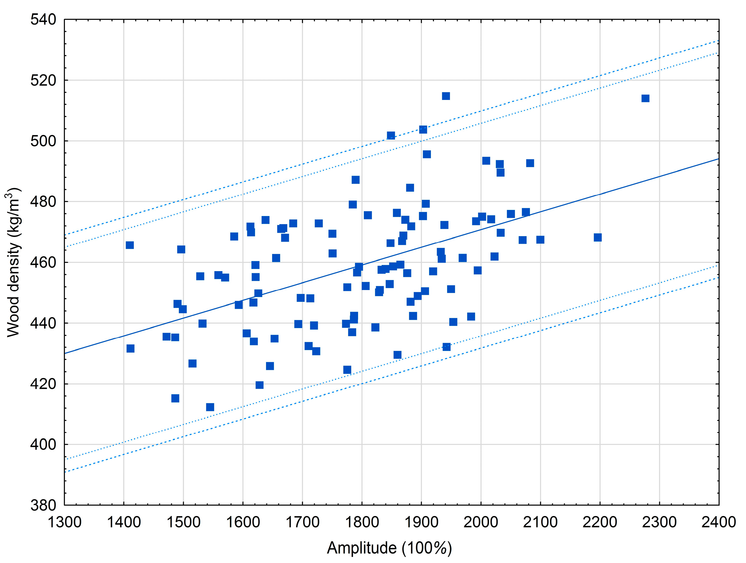
The resultant regression statistics and prediction error intervals for the relationship between mean amplitude and wood density are given in Table 6 and Table 7. Residual analyses indicated that there was insufficient evidence to reject the OLS assumptions of homogeneity of variance and normality. Figure 2 graphically illustrates the relationship in context of the calibration data set employed. Although the regression relationship described the observed linear trend adequately and there was no obvious systematic lack-of-fit (unbiasedness) present, only a relatively low proportion of the variability in wood density was explained by the relationship (r2 = 0.27; Table 6). The mean biases were not significantly different from zero as indicated by the 95% confidence intervals (Table 7), thus reconfirming the unbiased nature of the relationship. The prediction intervals indicated that the error generated from a newly sampled tree would be within 8% of its true value and that 95% of the errors generated from a large number of newly sampled trees would also be within 8% of their true value (Table 7).
3.2. Predictive Performance when Using an Acoustic-Based Estimate of Wood Density
Conceptually, the standard error of the estimate of the parameterized regressions indirectly provides a measure of estimation error: 95% of the errors would be expected to fall within 2 standard errors of the estimate of the true value. By contrast, the prediction and tolerance error intervals attempt to quantify the range of error that could arise when actually using the relationships to predict fibre attributes for a single or multiple number of newly sampled trees. For example, the prediction interval for me indicated that a single estimate for a newly measured tree would be would be within ±1.3 GPa of its true value, and that 95% of all errors from repeatedly sampling an infinite number of new trees would be within ±1.5 GPa of their true values (Table 5). These error ranges are applicable when sampling trees in which a Silviscan-based estimate of wood density is used. Realistically, however, such estimates would not be readily available and hence an alternative density estimate would be required. The results of this study suggest that either an acoustic- or Resistograph- based estimate could be used: wd = or wd = as presented in Table 4 and Table 6, respectively, and illustrated in Figure 1 and Figure 2, respectively. Although it was not possible to access the predictive ability of the Resistograph approach when used to estimate the attributes, the data set did enable an assessment of the density-weighted models when an acoustic-based wood density estimate is utilized as a surrogate measure for the Silviscan-based estimate: i.e., me, wt, co, sa = where is derived from the wd − relationship. Furthermore, in order to provide some context as to the performance of these relationships when used to estimate a mean population-based value, prediction ability was assessed at both the individual tree and stand level.
Computationally, this involved calculating the prediction error intervals arising from either sampling a single new tree or a group of new trees (n = 30). As presented in Table 8, the results indicated that there was no evidence of lack-of-fit for any of the relationships irrespective of error type: mean absolute and relative biases were not significantly (p ≤ 0.05) different from zero as inferred from the 95% confidence intervals. In terms of prediction error, the intervals indicated that there was a 95% probability that the absolute error for a newly sampled red pine tree when deploying and acoustic-based density estimate would fall within the following attribute-specific intervals (Table 8): −1.5 ≤ me error (GPa) ≤ 1.5; −0.3 ≤ wt error (µm) ≤ 0.3; −47.3 ≤ co error (µg/m) ≤ 47.3; and −23.1 ≤ sa error (m2/kg) ≤ 23.1. The corresponding relative intervals were as follows (Table 8): −12.5 ≤ me error (%) ≤ 13.0; −10.5 ≤ wt error (%) ≤ 10.9; −9.4 ≤ co error (%) ≤ 9.8; and −8.2 ≤ sa error (%) ≤ 8.4.
At the stand-level, the prediction intervals for absolute error when using an acoustic-based density estimate, indicated that there was a 95% probability that the mean of 30 future errors would fall within the following attribute-specific intervals (Table 8): −0.3 ≤ me error (GPa) ≤ 0.3; −0.1 ≤ wt error (µm) ≤ 0.1; −10.6 ≤ co error (µg/m) ≤ 10.7; and −5.2 ≤ sa error (m2/kg) ≤ 5.2. The corresponding relative intervals indicated the stand-level mean errors would fall within the following intervals: −2.6 ≤ me error (%) ≤ 3.2; −2.2 ≤ wt error (%) ≤ 2.6; −2.0 ≤ co error (%) ≤ 2.4; and −1.8 ≤ sa error (%) ≤ 1.9. The tolerance error intervals indicated that there was a 95% probability that 95% of all future errors generated from the use of an acoustic-based density estimate in the me, wd, wt, co and sa equations would fall within the following absolute and relative intervals: (1) −1.7 ≤ me error (GPa) ≤ 1.7; −0.4 ≤ wt error (µm) ≤ 0.4; −55.1 ≤ co error (µg/m) ≤ 55.1; and −26.9 ≤ sa error (m2/kg) ≤ 26.9; and (2) −14.7 ≤ me error (%) ≤ 15.2; −12.3 ≤ wt error (%) ≤ 12.6; −11.0 ≤ co error (%) ≤ 11.4; and −9.5 ≤ sa error (%) ≤ 9.6.
4. Discussion
End-product type and associated quality of an individual softwood tree is a function of its external morphological characteristics (e.g., stem diameter, height, sweep and taper, and the number and size of biotic and abiotic branches), and internal anatomical characteristics of the xylem tissue (e.g., modulus of elasticity, density, microfibril angle, tracheid wall thickness, radial and tangential tracheid diameters, fibre coarseness and specific surface area). Red pine produces a wide array of economically-important end-products which includes appearance-based boards used for interior flooring, exterior decking and wall panelling, dimensional lumber for residential home construction, utility poles used in building electrical transmission grids, veneer logs used in furniture manufacturing, and raw fibre for pulp for paper production and engineered wood composites [37]. Consequently, estimating end-product potential before harvest could provide the prerequisite knowledge for increasing segregation and merchandizing efficiency within the upstream portion of the forest products supply chain.
More specifically, based on an examination of the relationship between acoustic velocity and a suite of commercially-relevant red pine fibre attributes, the results of this study indicated that 5 of the 8 attributes studied, could be non-destructively estimated from time-of-flight acoustic velocity measurements. Contrary to expectation, the results for the relationship where microfibril angle is expressed as a function of density-weighted acoustic velocity revealed no graphical or statistical support for such a relationship. Microfibril angle and the dynamic modulus of elasticity are inversely proportional as empirically evident by the significance and multitude of the correlation between these attributes for the 54 red pine trees analyzed in this study (i.e., r = −0.81 (p ≤ 0.05); Table 2). Furthermore, other investigations have reported significant relationships between microfibril angle and acoustic velocity (e.g., [17,38]). Thus the results reported here for red pine should be considered tentative and suggest that additional research should be initiated in order to arrive at a more conclusive determination of the microfibril angle - acoustic velocity relationship for this species. (e.g., determining and accounting for potential covariates that could be influencing the relationship).
Collectively, based on a set of goodness-of-fit, lack-of-fit and predictive ability criteria, the results of this study indicated that viable relationships could be obtained for me, wd, wt, co and sa. Specifically, based on their statistical significance (p ≤ 0.05; Table 4), proportion of variability explained (40%, 14%, 45%, 27% and 43% of the variation in me, wd, wt, co and sa explained, respectively; Table 4), and predictive precision (e.g., 95% of all future errors would be within 12%, 8%, 7%, 8% and 6% of the true value of me, wd, wt, co and sa, respectively; Table 5)). Furthermore, given that a wood density estimate is required for deploying the me, wt, co and sa relationships, two non-destructive approaches for estimating wd were also evaluated (acoustic and micro-drill resistance measures). Results from these analyses indicated that both approaches could provide unbiased wood density estimates at moderate levels of precision (e.g., ±8%; Table 5 and Table 7). Combining the acoustic-based density estimates with the parameterized functions revealed that me, wt, co and sa could be unbiasedly predicted at moderate levels of precision at the individual tree level and at relatively high levels of precision for stand-level mean values (Table 8): (1) the future error arising from me, wt, co or sa prediction for a newly sampled tree would be expected to fall within 13%, 11%, 10% and 8%, respectively, of their true values; and (2) mean error arising from me, wt, co or sa predictions for a newly sampled stand of trees would be expected to fall within 3%, 2%, 2% and 2%, respectively, of their true values.
4.1. The Acoustic Velocity-Stiffness Relationship and Associated Inferences
The relationship between the modulus of elasticity and the density-weighted acoustic velocity of a mechanically-induced dilatational stress wave within standing trees was originally derived from engineering principles and subsequently empirically validated through field and laboratory experimentation [39,40]. Practically, however, the relationship is difficult to apply in the field given the logistical challenges of estimating wood density non-destructively. Thus, apart from a few studies that have incorporated surrogate measures of density obtained through the use of non-destructive tools such as the Resistograph (this study) or the Pilodyn (PROCEQ, Zurich, Switzerland; [41]), most previous studies have either omitted the density term or assumed that it is an invariant species or sample specific constant. Analytically comparable studies to this study, such as that completed by Chen [41], reported a significant (p ≤ 0.05) but weak relationship (r2 = 0.28) in this regard for Norway spruce (Picea abies (L.) Karst.). Contrasting this result with that obtained for red pine, likewise exhibited a significant (p ≤ 0.05) but slightly higher descriptive relationship (r2 = 0.42). Other studies employing the simpler density-unweighted acoustic velocity variable, have reported a considerable range in the proportion of variation explained by the stiffness - acoustic velocity relationship: coefficients of determination have ranged from 0.11 to 0.41 [39]. More complex regression models in which presumed covariates affecting acoustic velocity have been incorporated, have also been proposed. Although one of the most frequent covariates considered is tree size (diameter at breast-height), results have been mixed in terms of its influence in increasing the proportion of variability explained when included in specifications derived from Equation (1) [15]. Analyzing the data for the 54 red pine trees assessed in this study, indicated no significant correlation between acoustic velocity and breast-height diameter (i.e., r = −0.018 (p > 0.05)), thus providing confirmatory support for the deployment of the more classical representation of the modulus of elasticity − acoustic velocity relationship (sensu Equation (1)).
Previous studies have assessed the direct relationship between the dynamic me of standing trees and the corresponding static me of the resultant end-products as determined via the bending stress tests of dimensional lumber or laboratory assessment of clear wood specimens extracted from sawn boards. Overall, the strength of these relationships as measured by the degree of correlation or the proportion of variation explained, has also varied among studies. For example, Amateis and Burkhart [42] found a non-significant (p > 0.05) relationship between time-of-flight acoustic velocity impulses within standing loblolly pine (Pinus taeda L.) trees and the static modulus of elasticity of the resultant sawn boards. Chen [41] and Fischer [43] reported significant (p ≤ 0.05) but relatively weak relationships in this regard for Norway spruce (r2 values of 0.25 and 0.13, respectively). Conversely, Wang [12] reported significant and relatively moderately strong relationships for western hemlock (Tsuga heterophylla (Raf.) Sarg.; r2 = 0.73) and Sitka spruce (Picea sitchensis (Bong.) Carr.); r2 = 0.77).
This wide range of results among studies in terms of the significance and strength of the relationships is partially due to differences among the investigations in terms of the species examined, sampling protocols used, environmental conditions at the time of measurements (e.g., seasonal differences in temperature and moisture), locale, instrumentation (e.g., Director ST300 or TreeSonic acoustic velocity tools; Resistograph or the Pilodyn (PROCEQ, Zurich, Switzerland) wood density estimation tools), model specifications (e.g., density-unweighted or density-weighted acoustic velocity variable), correlation versus regression analysis, simple or multiple regression analyses), and availability of modulus of elasticity measures within clear wood samples from standing trees (e.g., this study) or from derived end-products (dimensional lumber). These differences are problematic in terms of drawing explicit comparisons among and between studies. Nevertheless, on a collective basis, the results presented in this study for standing red pine trees are in general agreement with the range of previous results in terms of statistical significance, explanatory performance and predictive ability. Thus providing further incremental empirical support for the generality of the relationship between density-weighted acoustic velocity and the dynamic modulus of elasticity for standing trees.
4.2. Standing Tree Versus Log Acoustic Relationships and a Poisson Ratio Estimate for Red Pine
Conceptually, the relationship between the dynamic modulus of elasticity and acoustic velocity varies between standing trees and sawn logs because the wave types being generated are different. For standing trees, it is the time-of-flight (velocity) of a mechanically-induced dilatational or quasi-dilatational stress wave that enters from the circumference of the stem just above stump height (0.3 m), progressing vertically through the xylem tissue which transects breast-height (1.3 m), and then exits the stem at a height of approximately 1.5 m. For logs, it is the velocity of a mechanically-induced resonance-based longitudinal stress wave that enters the log at one of its open cross-sectional faces (log ends), progressing horizontally through the xylem tissue until arriving at the opposite log face. Although the wave types differ along with their functional relationship with the modulus of elasticity, the velocity measurements are correlated. Specifically, Wang [17] reported that the mean ratio between the time-of-flight acoustic velocity estimate for standing trees (vd) and the resonance acoustic velocity estimate for butt logs (vl) for the same sample trees across 5 coniferous species, Sitka spruce (Picea sitchensis (Bong.) Carr.), western hemlock (Tsuga heterophylla (Raf.) Sarg), jack pine, ponderosa pine (Pinus ponderosa Dougl. ex Laws.), and radiata pine (Pinus radiata D. Don), ranged from 1.07 to 1.36 with a mean value of 1.20. Based on tree and log acoustic measures for the red pine trees considered in this study, results revealed an overall mean ratio of 1.39 with individual ratios ranging from a minimum of 1.28 to a maximum of 1.56.
Although tree and log velocities are not equivalent given that they are reflecting 2 different types of stress waves (dilatational for tree and longitudinal for logs), their inter-relationship can be used to empirically estimate the Poisson ratio, which is a principal covariate in the primary acoustic relationship (Equation (1)). Mechanically, the Poisson ratio represents the transverse to axial strain relationship when a wood sample is axially loaded (i.e., ratio of the deformation perpendicular to the direction of the load (transverse strain) is proportional to the deformation parallel to the direction of the load (axial strain)). Given that the Poisson ratio varies within and between species and is affected by the moisture content and specific gravity [44], it is commonly treated as an unknown constant when acoustically estimating wood stiffness. However, Wang [17] demonstrated an approach for empirically deriving the Poisson ratio (P) based on the ratio between vd and vl: specifically, by inputting a mean ratio value and subsequently solving for P in the relationship. Solving this relationship employing the acoustic ratio obtained for the red pine trees sampled in this study, yields an estimated P value of 0.39. This value is slightly greater than the largest value reported by Wang [17] (i.e., 0.38 for Ponderosa pine). More generally, however, a generic mean value of 0.37 is commonly assumed for both hardwoods and softwoods [45] and hence the acoustic-based empirical P estimate for red pine is not dissimilar. Irrespective of its numeric value relative to other species, provision of the P estimate could be of future utility when quantifying acoustic-based relationships for red pine.
4.3. A Suite of Acoustic Velocity-Attribute Relationships and their Potential Operational Utility
The conceptual expansion of the primary relationship to include secondary relationships, consequentially expands the acoustic-based analytical framework. These additional attributes provide for a much more comprehensive assessment of end-product potential than that based on stiffness alone. The empirical results obtained in this study for standing red pine trees, indicated that the acoustic velocity approach could be used to estimate wood density, tracheid wall thickness, fibre coarseness and specific surface area, in addition to the dynamic modulus of elasticity. This expanded set of attributes are associated with a wider range of end-products which can be used as surrogate indicators of potential end-product quality (Table 1). Results from a parallel analysis deploying a similar inferential framework for investigating the relationship between the same attributes used in this study and velocity of a mechanically-induced longitudinal stress wave but for red pine logs derived from the same sample trees as used in this study, were in accord with those found in this study [28]. Specifically, assessment of the relationship between acoustic velocity as measured via the Director HM200 acoustic velocity resonance tool (Fibre-gen Inc., Christchurch, New Zealand; www.fibre-gen.com) and the same 8 Silviscan-determined attributes as used in this study, revealed viable regression relationships for the same 5 variables based on statistical significance, unbiasedness and predictive ability (i.e., modulus of elasticity, wood density, cell wall thickness, fibre coarseness and specific surface area).
Operationally, the parameterized equations can be used to generate estimates for the dynamic modulus of elasticity, wood density, tracheid wall thickness, fibre coarseness and specific surface area within standing red pine trees (Table 4). In-forest implementation of the regression relationships will require an end-user to attain a prerequisite wood density estimate using either an acoustic velocity measurement obtained using the Director 300 time-of-flight tool (i.e., wd = ; Table 4; Figure 1), or from an amplitude measurement obtained using the Resistograph micro-drill tool (i.e., wd = ; Table 5; Figure 2). In regards to the latter approach, the assessment and quantification of the relationship between drill resistance amplitude and wood density represents an alternative field-based approach for obtaining a density estimate. The Resistograph measures the relative resistance (expressed as the percent amplitude) of a micro-diameter drill bit rotating at a constant rate and being inserted at a constant rate when drilled radially into a standing tree. Although designed for assessing the structural integrity of load-bearing wood-based structures including bridge supports, timber beams and utility poles, the Resistograph as shown in this study and by others (e.g., [46]), can provide an indirect estimate of wood density. The correlation between the mean amplitude value derived from drill resistance profiles and oven-dry wood density has varied across studies, ranging from a low of 0.29 to a high of 0.89 ([29,46], respectively). The result from this study for red pine falls midway within this range (r = 0.51; derived from Table 5) and hence is in general agreement with these previous findings. Thus, in addition to providing a species-specific parameterized equation for predicting density within standing red pine trees, the results of this analysis provide additional incremental support for the micro-drilling approach in wood density estimation.
From a logistical perspective, however, the acoustic approach is less complex to implement. Furthermore, deploying acoustic-based wood density estimates would yield unbiased individual and stand-level attribute estimates at generally tolerable levels of precision. For example, at the individual tree-level, there was a 95% probability that a future error arising from the prediction of me, wt, co and sa using a newly acquired acoustic velocity measurement for an individual red pine tree along with the corresponding acoustic-based density estimates, would be within 13%, 11%, 10% and 8% of their true values, respectively (Table 8). At the stand-level, there was a 95% probability that the mean error arising from the prediction of me, wt, co and sa using 30 newly acquired acoustic velocity measurements from a stand of trees along with the corresponding acoustic-based density estimates, would be within 3%, 2%, 2% and 2% of their true values, respectively (Table 8). More generally, the tolerance intervals indicated that 95% of all future errors would be within 15%, 12%, 11% and 10% of their true me, wt, co and sa values, respectively (Table 8).
The utility of the acoustic approach for in-forest segregation of individual trees into end-product categories and associated grade classes based on the me, wd, wt, co or sa estimates, is ultimately dependent on the accuracy requirements of the end-user. The precision of the acoustic-based estimates for red pine as quantified by the prediction and tolerance error intervals can provide operational guidance for such a determination. For example, the mean difference for the static me between the 14 consecutive machine stress-rated lumber grades for conifers is approximately 0.7 GPa, according to the National Lumber Grades Authority [11]. However, the prediction interval for an acoustic-based dynamic me estimate for an individual red pine tree is ±1.5 GPa (Table 8). Thus, even if one assumed a 1-to-1 relationship between dynamic elasticity estimates in standing trees and static elasticity estimates within derived dimensional lumber products, the acoustic-based stiffness estimates would not be precise enough to sort standing trees into grade classes requiring such a ±0.7 GPa precision level. Alternatively, grouping the grade categories into a smaller set of discrete classes may be a viable approach. Based on the NLGA [47] machine stress-rated lumber specifications for spruce, pine and fir boards, Paradis [48] used 3 me-based grade classes to represent lumber end-product potentials for black spruce. These 3 classes, denoted low, medium and high grade, were differentiated by approximately 1.5 me units (GPa), and hence if similarly applied to red pine, the acoustic-based dynamic me estimate would be precise enough to segregate individual trees into one of these 3 classes.
The lack of specific design specifications for the other predictable attributes (wood density, cell wall thickness, fibre coarseness and specific surface area) negates a similar assessment of the potential utility of the estimates to explicitly differentiate standing red pine trees into discrete end-product quality classes. However, assessing individual trees or stands using all the of the estimable attributes collectively, affords the end-user the ability to segregate standing red pine trees into coarse-level end-product-based categories (sensu Table 1). For example, the solid wood end-product potential of standing trees could be determined from the modulus of elasticity and wood density estimates given that these attributes are directly proportional to lumber stiffness and strength, respectively. Conversely, the pulp and paper end-product potential of standing red pine trees could be inferred from the wall thickness, fibre coarseness and specific surface area estimates, given that these estimates are inversely proportional to the tensile strength, directly proportional to tear strength and inversely proportional to yield of derived paper products, respectively.
The expansion of the acoustic approach to estimate additional internal wood attributes along with provision of the prerequisite prediction equations, provides the foundation for potentially deploying an expanded inferential framework in red pine segregation operations. In terms of further research, it would be advantageous to direct efforts towards identifying and minimizing potential sources of variation influencing the attribute-specific acoustic relationships, and establishing quantitative linkages between within-tree and within-product attribute estimates. For example, establishing species-specific relationships between acoustic-based dynamic modulus of elasticity estimates within standing trees and mechanical-based static modulus of elasticity estimates within derived solid wood products, would improve in-forest end-product forecasts and provide more precise wood property characterization of the raw material before merchandizing (sensu [49]). Ultimately, such efforts could potentially yield a more comprehensive and precise end-product segregation protocol resulting in improved in-forest decision-making within the upstream portion of the red pine forest products supply chain.
5. Conclusions
End-product potential and quality are directly associated with the internal fibre attributes of individual trees. Hence, the ability to identify and segregate standing trees according to these attributes via the use of acoustic-based non-destructive sampling methods, enables the forecasting of end-product potential of individual trees or stands before harvest. Considering that red pine produces a wide array or economically-important products, differentiating standing trees according to their end-product potential could increase the likelihood of optimizing allocation and merchandizing decisions. The results of this study provide empirical support for the potential use of acoustic-based methods in estimating a suite of commercially-relevant fibre attributes for standing red pine trees. Specifically, based on a set of statistical-based measures, viable prediction models were developed for 5 of the 8 attributes considered (dynamic modulus of elasticity, wood density, tracheid wall thickness, fibre coarseness and specific surface area). Although these results are promising, further research in terms of broadening existing end-product type and associated grade definitions based on a broader suite of attribute-specific determinants, and identifying and controlling consequential sources of variation during acoustic-based field sampling, will be required before the full potential of the non-destructive acoustic-based approach to wood quality characterization is realized.
Acknowledgments
The author expresses his appreciation to (1) Mike Laporte (retired) of the Canadian Wood Fibre Centre (CWFC, Canadian Forest Service, Natural Resources Canada), Sault Ste. Marie, ON, Canada, for his assistance in the field data acquisition and laboratory processing activities; (2) logging machine operators and planning staff from Thomas Woods Development Inc., Bruce Mines, ON, Canada, for felling and sectioning the 54 sample trees; (3) Dr. Tong, Dr. Woo and Nelson Ny at FPInnovation Inc., Vancouver, BC, Canada, for conducting the SilviScan-3 analyses; (4) Unit Forestry Staff from the Ontario Ministry of Natural Resources and Forestry office in Blind River, ON, Canada, for assistance in accessing the historical archives relating to the Kirkwood Forest; (5) Dr. Sharma of the Ontario Forest Research Institute, Sault Ste. Marie, ON, Canada, for providing access to regulated refrigeration facilities for disk storage; (6) CWFC for fiscal support; and (7) anonymous journal reviewers for their constructive and insightful comments and suggestions.
Conflicts of Interest
The author declares no conflict of interest.
References
- Emmett, B. Perspectives on sustainable development and sustainability in the Canadian forest sector. For. Chron. 2006, 82, 40–43. [Google Scholar] [CrossRef]
- Wegner, T.; Skog, K.E.; Ince, P.J.; Michler, C.J. Uses and desirable properties of wood in the 21st Century. J. For. 2010, 108, 165–173. [Google Scholar]
- Nilsson, S. Transition of the Canadian forest sector. In The Future Use of Nordic Forests—A Global Perspective; Westholm, E., Lindahl, K.B., Kraxner, F., Eds.; Springer: Cham, Switzerland, 2015; pp. 125–144. [Google Scholar]
- Ontario Ministry of Natural Resources and Forestry (OMNRF). Forest Management Guide to Silviculture in the Great Lakes-St. Lawrence and Boreal Forests of Ontario; Queens Printer for Ontario: Toronto, ON, Canada, 2015.
- Newton, P.F. A decision-support system for forest density management within upland black spruce stand-types. Environ. Model. Softw. 2012, 35, 171–187. [Google Scholar] [CrossRef]
- I’Anson, S.J.; Karademir, A.; Sampson, W.W. Specific contact area and the tensile strength of paper. Appita 2006, 59, 297–308. [Google Scholar]
- Bowyer, J.L.; Shmulsky, R.; Haygreen, J.G. Forest Products and Wood Science: An Introduction, 5th ed.; Blackwell Publishing: Ames, IA, USA, 2007. [Google Scholar]
- Hong, Z.; Fries, A.; Lunqvist, S.-O.; Gull, B.A.; Wu, H.X. Measuring stiffness using acoustic tool for Scots pine breeding selection. Scand. J. For. Res. 2015, 30, 363–372. [Google Scholar] [CrossRef]
- Mora, C.R.; Schimleck, L.R.; Isik, F.; Mahon, J.M.; Clark, A., Jr.; Daniels, R.F. Relationships between acoustic variables and different measures of stiffness in standing Pinus taeda trees. Can. J. For. Res. 2009, 39, 1421–1429. [Google Scholar] [CrossRef]
- Gao, S.; Wang, X.; Wiemann, M.C.; Brashaw, B.K.; Ross, R.J.; Wang, L. A critical analysis of methods for rapid and non-destructive determination of wood density in standing trees. Ann. For. Sci. 2017, 74, 1–15. [Google Scholar] [CrossRef]
- National Lumber Grades Authority (NLGA). Standard Grading Rules for Canadian Lumber; National Lumber Grades Authority (NLGA): Surrey, BC, Canada, 2014. [Google Scholar]
- Wang, X.; Ross, R.J.; McClellan, M.; Barbour, R.J.; Erickson, J.R.; Forsman, J.W.; McGinnis, G.D. Nondestructive evaluation of standing trees with a stress wave method. Wood Fiber Sci. 2001, 33, 522–533. [Google Scholar]
- Raymond, C.A.; Joe, B.; Evans, R.; Dickson, R.L. Relationship between timber grade, static and dynamic modulus of elasticity, and Silviscan properties for Pinus radiata in New South Wales. N. Z. J. For. Sci. 2007, 37, 186–196. [Google Scholar]
- Divós, F.; Tanaka, T. Relation between static and dynamic modulus of elasticity of wood. Acta Silv. Lignaria Hung. 2005, 1, 105–110. [Google Scholar]
- Legg, M.; Bradley, S. Measurement of stiffness of standing trees and felled logs using acoustics: A review. J. Acoust. Soc. Am. 2016, 139, 588–604. [Google Scholar] [CrossRef] [PubMed]
- Bucur, V. Acoustics of Wood, 2nd ed.; Springer: Berlin, Germany, 2006. [Google Scholar]
- Wang, X.; Ross, R.J.; Carter, P. Acoustic evaluation of wood quality in standing trees. Part I. Acoustic wave behavior. Wood Fiber Sci. 2007, 39, 28–38. [Google Scholar]
- Essien, C.; Cheng, Q.; Via, B.K.; Loewenstein, E.F.; Wang, X. An acoustics operations study for Loblolly pine (Pinus taeda) standing saw timber with different thinning history. Bioresources 2016, 11, 7512–7521. [Google Scholar] [CrossRef]
- Filipescu, C.N.; Trofymow, J.A.; Koppenaal, R.S. Late-rotation nitrogen fertilization of Douglas-fir: Growth response and fibre properties. Can. J. For. Res. 2017, 47, 134–138. [Google Scholar] [CrossRef]
- Lasserre, J.P.; Mason, E.; Watt, M. The influence of initial stocking on corewood stiffness in a clonal experiment on 11-year-old Pinus radiata D. Don. N. Z. J. For. Sci. 2004, 49, 18–23. [Google Scholar]
- Wang, X.; Carter, P.; Ross, R.J.; Brashaw, B.K. Acoustic assessment of wood quality of raw materials: A path to increased profitability. For. Prod. J. 2007, 57, 6–14. [Google Scholar]
- Evans, R. Rapid measurement of the transverse dimensions of tracheids in radial wood sections from Pinus radiata. Holzforschung 1994, 48, 168–172. [Google Scholar] [CrossRef]
- Evans, R.; Stuart, S.A.; Van Der Touw, J. Microfibril angle scanning of increment cores by X-ray diffractometry. Appita 1996, 49, 411–414. [Google Scholar]
- Evans, R. Wood stiffness by X-ray diffractometry. In Characterization of the Cellulosic Cell Wall; Stokke, D.D., Groom, L.H., Eds.; Wiley: Hoboken, NJ, USA, 2006; pp. 138–146. [Google Scholar]
- Newton, P.F. Predictive relationships between acoustic velocity and wood quality attributes within standing jack pine trees. In preparation.
- Rowe, J.S. Forest Regions of Canada; Publication No. 1300; Government of Canada, Department of Environment, Canadian Forestry Service: Ottawa, ON, Canada, 1972.
- Newton, P.F. Development trends of black spruce fibre attributes in maturing plantations. Int. J. For. Res. 2016, 1–12. [Google Scholar]
- Newton, P.F. Predictive relationships between acoustic velocity and wood quality attributes for red pine logs. For. Sci. 2017, 63, 504–517. [Google Scholar] [CrossRef]
- Rinn, F.; Schweingruber, R.H.; Schär, E. Resistograph and X-ray density charts of wood. Comparative evaluation of drill resistance profiles and x-ray density charts of different wood species. Holzforschung 1996, 50, 303–311. [Google Scholar] [CrossRef]
- Wilson, F.G. Numerical expression of stocking in term of height. J. For. 1946, 44, 758–761. [Google Scholar]
- Pierpoint, G. The Sites of the Kirkwood Management Unit; Report 47; Research Branch, Department of Lands and Forests: Toronto, ON, Canada, 1962. [Google Scholar]
- Beckwith, A.F.; Roebbelen, P.; Smith, V.G. Red pine Plantation Growth and Yield Tables; Forest Research Report No. 108; Ontario Ministry of Natural Resources: Maple, ON, Canada, 1983.
- Defo, M.; Goodison, A.; Nelson, U. A method to map within-tree distribution of fibre properties using SilviScan-3 data. For. Chron. 2009, 85, 409–414. [Google Scholar] [CrossRef]
- Neter, J.; Wasserman, W.; Kutner, M.H. Applied Linear Statistical Models, 3rd ed.; Irwin: Boston, MA, USA, 1990. [Google Scholar]
- Reynolds, M.R., Jr. Estimating the error in model predictions. For. Sci. 1984, 30, 454–469. [Google Scholar]
- Gribbo, L.S.; Wiant, H.V., Jr. A SAS template program for the accuracy test. Compiler 1992, 10, 48–51. [Google Scholar]
- Zhang, S.Y.; Koubaa, A. Softwoods of Eastern Canada: Their Silvics, Characteristics, Manufacturing and End-Uses; Special Publication SP-526E; FPInnovations: Quebec, QC, Canada, 2008. [Google Scholar]
- Evans, R.; Ilic, J. Rapid prediction of wood stiffness from microfibril angle and density. For. Prod. J. 2001, 51, 53–57. [Google Scholar]
- Wessels, C.B.; Malan, F.S.; Rypstra, T. A review of measurement methods used on standing trees for the prediction of some mechanical properties of timber. Eur. J. For. Res. 2011, 130, 881–893. [Google Scholar] [CrossRef]
- Wang, X. Acoustic measurements on trees and logs: A review and analysis. Wood Sci. Technol. 2013, 47, 965–975. [Google Scholar] [CrossRef]
- Chen, Z.-Q.; Karlsson, B.; Lundqvist, S.-O.; Gil, M.R.G.; Olsson, L.; Wu, H.X. Estimating solid wood properties using Pilodyn and acoustic velocity on standing trees of Norway spruce. Ann. For. Sci. 2015, 72, 499–508. [Google Scholar] [CrossRef]
- Amateis, R.L.; Burkhart, H.E. Use of the Fakopp TreeSonic acoustic device to estimate wood quality characteristics in loblolly pine trees planted at different densities. In Proceedings of the 17th Biennial Southern Silvicultural Research Conference, Asheville, NC, USA, 2015; pp. 519–522. [Google Scholar]
- Fischer, C.; Vestøl, G.I.; Øvrum, A.; Høibø, O.A. Pre-sorting of Norway spruce structural timber using acoustic measurements combined with site-, tree- and log characteristics. Eur. J. Wood Prod. 2015, 73, 819–828. [Google Scholar] [CrossRef]
- Green, D.W.; Winandy, J.E.; Kretschmann, D.E. Wood as an Engineering Material; General Technical Report FPL-GTR-113; USDA Forest Service: Madison, WI, USA, 1999.
- Bodig, J.; Goodman, J.R. Prediction of elastic parameters of wood. Wood Sci. 1973, 5, 249–264. [Google Scholar]
- Isik, F.; Li, B. Rapid assessment of wood density of live trees using the Resistograph for selection in tree improvement programs. Can. J. For. Res. 2003, 33, 2426–2435. [Google Scholar] [CrossRef]
- National Lumber Grades Authority (NLGA). Special Products Standard for Machine Graded Lumber; National Lumber Grades Authority (NLGA): Surrey, BC, Canada, 2003. [Google Scholar]
- Paradis, N.; Auty, D.; Carter, P.; Achim, A. Using a standing-tree acoustic tool to identify forest stands for the production of mechanically-graded lumber. Sensors 2013, 13, 3394–3408. [Google Scholar] [CrossRef] [PubMed]
- Bachtiar, E.V.; Sanabria, S.J.; Mittig, J.P.; Niemz, P. Moisture-dependent elastic characteristics of walnut and cherry wood by means of mechanical and ultrasonic test incorporating three different ultrasound data evaluation techniques. Wood Sci. Technol. 2017, 51, 47–67. [Google Scholar] [CrossRef]
Figure 1.
Attribute-specific acoustic-based relationships with significant (p ≤ 0.05) regression relationships superimposed (solid line; Table 4): , , , , , , and . Contextual 95% prediction and tolerance intervals for absolute error are also superimposed for the significant relationships: dotted and dashed parallel lines, respectively (Table 5).
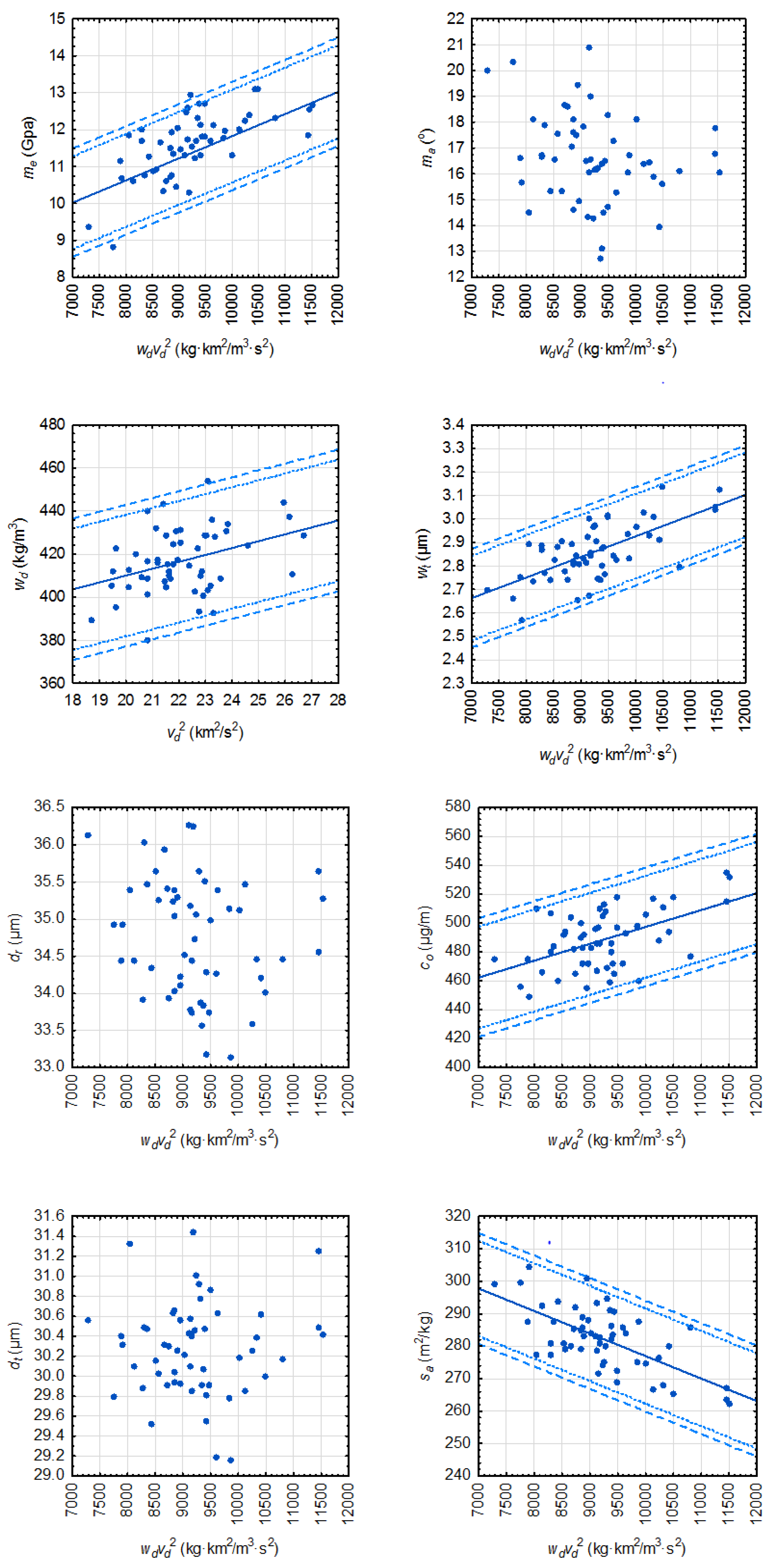
Figure 2.
Relationship between mean amplitude and wood density with regression relationship superimposed (solid line; Table 6). Contextual 95% prediction and tolerance intervals for absolute error are also superimposed: dotted and dashed parallel lines, respectively (Table 6 and Table 7).

Table 1.
Wood product-based performance measures and their relationship with fibre attributes (sensu [6,7]).
| Product Category | Performance Measure | Relationship with Fibre Attribute |
|---|---|---|
| Pulp | Tensile strength | specific surface area, (wall thickness)−1 |
| and | Tear strength | fibre length, coarseness |
| paper | Stretch | microfibril angle |
| Bulk | wall thickness, (fibre width)−1 | |
| Light scattering | (wall thickness)−1 | |
| Collapsibility | wall thickness | |
| Solid wood, | Strength | density, (microfibril angle)−1 |
| wood composites and utility poles | Stiffness | density, modulus of elasticity, (microfibril angle)−1 |
Table 2.
Species-specific bivariate linear associations between Silviscan-determined accumulative area-weighted mean fibre attributes: Pearson product moment correlation coefficients for the relationship between the dynamic modulus of elasticity and commercially-relevant secondary attributes for 50 semi-mature black spruce trees [27], 61 semi-mature jack pine trees [25] and 54 mature red pine trees (this study).
| Attribute | Modulus of Elasticity | ||
|---|---|---|---|
| Black Spruce | Jack Pine | Red Pine | |
| Wood density | 0.777 * | 0.672 * | 0.759 * |
| Microfibril angle | −0.898 * | −0.710 * | −0.808 * |
| Tracheid wall thickness | 0.677 * | 0.665 * | 0.687 * |
| Radial tracheid diameter | −0.448 * | −0.317 * | −0.383 * |
| Tangential tracheid diameter | −0.304 * | −0.081 | −0.089 |
| Fibre coarseness | 0.204 | 0.541 * | 0.439 * |
| Specific surface area | −0.581 * | −0.637 * | −0.636 * |
Note: * denotes a significant correlation at the 0.05 probability level.
Table 3.
Descriptive statistical summary of the mensurational characteristics, acoustic velocity measurements and cumulative area-weighted fibre attributes for the 54 standing sample trees.
Table 3.
Descriptive statistical summary of the mensurational characteristics, acoustic velocity measurements and cumulative area-weighted fibre attributes for the 54 standing sample trees.
| Variable | Unit | Mean | Standard Error | Minimum | Maximum | CV a (%) |
|---|---|---|---|---|---|---|
| Diameter at breast-height | cm | 38.0 | 0.51 | 30.7 | 46.5 | 9.8 |
| Breast-height age | year | 77 | 0.32 | 73 | 81 | 3.0 |
| Total height | m | 27.8 | 0.17 | 23.8 | 30.0 | 4.4 |
| Live crown ratio | % | 34.1 | 0.83 | 24.9 | 51.7 | 18.0 |
| Dilatational stress wave velocity (vd) | km/s | 4.70 | 0.02 | 4.33 | 5.17 | 3.9 |
| Modulus of elasticity (me) | GPa | 11.6 | 0.13 | 8.8 | 13.1 | 8.1 |
| Wood density (wd) | kg/m3 | 416.9 | 2.04 | 378.0 | 454.3 | 3.6 |
| Microfibril angle (ma) | ° | 16.6 | 0.23 | 12.7 | 20.9 | 10.4 |
| Tracheid wall thickness (wt) | µm | 2.86 | 0.02 | 2.57 | 3.1 | 4.2 |
| Tracheid radial diameter (dr) | µm | 34.8 | 0.11 | 33.1 | 36.3 | 2.3 |
| Tracheid tangential diameter (dt) | µm | 30.3 | 0.06 | 29.2 | 31.5 | 1.6 |
| Coarseness (co) | µg/m | 488.5 | 2.78 | 449.2 | 535.5 | 4.2 |
| Specific surface area (sa) | m2/kg | 282.3 | 1.31 | 262.3 | 304.4 | 3.4 |
a Coefficient of variation.
Table 4.
Parameter estimates and regression statistics for each attribute-specific acoustic-based relationship (Equation (3)).
Table 4.
Parameter estimates and regression statistics for each attribute-specific acoustic-based relationship (Equation (3)).
| Relationship | Parameter Estimates a | Regression Statistics b | ||||
|---|---|---|---|---|---|---|
| Intercept | Slope | df | r2 | SEE | F-Ratio | |
| (nreg, nres) | ||||||
| 5.823 | 0.0006 | 1, 51 | 0.422 | 0.676 | 37.3 * | |
| 346.093 | 3.1981 | 1, 52 | 0.137 | 14.080 | 8.3 * | |
| 20.706 | −0.0004 | 1, 52 | 0.055 | 1.688 | 3.0 ns | |
| 2.047 | 0.0001 | 1, 52 | 0.446 | 0.090 | 41.9 * | |
| 36.242 | −0.0002 | 1, 52 | 0.033 | 0.797 | 1.8 ns | |
| 30.086 | 0.0000 | 1, 52 | 0.002 | 0.475 | 0.1 ns | |
| 380.522 | 0.0117 | 1, 52 | 0.270 | 17.604 | 19.2 * | |
| 346.339 | −0.0069 | 1, 52 | 0.430 | 7.314 | 39.2 * | |
a OLS parameter estimates for the intercept and slope (Equation (3)); b Degrees of freedom (df) for regression (nreg) and residual error (nres), coefficient of determination (r2) and standard error of the estimate (SEE where units are specific to the dependent variable: GPa, kg/m3, °, µm, µm, µm, µg/m and m2/kg for me, wd, ma, wt, dr, dt, co and sa, respectively), and F-statistic where superscripts * and ns denote a significant (p ≤ 0.05) or non-significant (p > 0.05) relationship, respectively.
Table 5.
Lack-of-fit and predictive ability metrics for each significant attribute-specific acoustic-based relationship.
Table 5.
Lack-of-fit and predictive ability metrics for each significant attribute-specific acoustic-based relationship.
| Relationship | Lack-of-Fit Measures a | Predictive Ability: 95% Error Intervals c | ||||||
|---|---|---|---|---|---|---|---|---|
| Absolute b | Relative (%) | Prediction | Tolerance | |||||
| Mean Bias | 95% CL | Mean Bias | 95% CL | Absolute b | Relative (%) | Absolute b | Relative (%) | |
| 95% CL | 95% CL | 95% CL | 95% CL | |||||
| 0.000 | ±0.173 | 0.289 | ±1.511 | ±1.258 | ±11.003 | ±1.469 | ±12.854 | |
| 0.000 | ±3.807 | 0.110 | ±0.916 | ±28.237 | ±6.794 | ±32.894 | ±7.915 | |
| 0.000 | ±0.024 | 0.096 | ±0.858 | ±0.180 | ±6.361 | ±0.210 | ±7.410 | |
| 0.000 | ±4.761 | 0.126 | ±0.983 | ±35.305 | ±7.289 | ±41.128 | ±8.492 | |
| 0.000 | ±1.978 | 0.064 | ±0.696 | ±14.669 | ±5.161 | ±17.088 | ±6.012 | |
a Mean absolute (Equation (5)) and relative (Equation (6)) bias and the limits of the associated 95% confidence interval (CL; Equation (7)) where mean values not significantly (p > 0.05) different from zero were indicative of an unbiased relationship; b Absolute error units are attribute-specific: GPa, kg/m3, µm, µg/m and m2/kg for me, wd, wt, co and sa, respectively; c Confidence limits (CL) for the 95% prediction and tolerance intervals for absolute and relative errors (Equations (8) and (9), respectively): mean bias ±95% CL. Specifically, there is a 95% probability that a future error will be within the stated prediction interval and that there is a 95% probability that 95% of all future errors will be within the stated tolerance interval [35,36].
Table 6.
Parameter estimates and regression statistics for the relationship between mean amplitude and wood density.
Table 6.
Parameter estimates and regression statistics for the relationship between mean amplitude and wood density.
| Parameter Estimates and Regression Statistics | |||||
|---|---|---|---|---|---|
| Parameter | Regression Statistics b | ||||
| Estimates a | df | r2 | SEE | F-ratio | |
| Intercept | Slope | (nreg, nres) | (kg/m3) | ||
| 354.184 | 0.0583 | 1104 | 0.265 | 17.644 | 37.5 * |
a Ordinary least squares parameter estimates for the intercept and slope (Equation (4)); b Degrees of freedom (df) for regression (nreg) and residual error (nres), coefficient of determination (r2) and standard error of the estimate (SEE where units are specific to the dependent variable: GPa, kg/m3, °, µm, µm, µm, µg/m and m2/kg for me, wd, ma, wt, dr, dt, co and sa, respectively), and F-statistic where superscripts * and ns denote a significant (p ≤ 0.05) or non-significant (p > 0.05) relationship, respectively.
Table 7.
Lack-of-fit and prediction error metrics for the relationship between mean amplitude and wood density.
Table 7.
Lack-of-fit and prediction error metrics for the relationship between mean amplitude and wood density.
| Lack-of-Fit Measures a | Predictive Ability: 95% Error Intervals b | ||||||
|---|---|---|---|---|---|---|---|
| Absolute | Relative | Prediction | Tolerance | ||||
| Mean | 95% CL | Mean | 95% CL | Absolute | Relative | Absolute | Relative |
| (kg/m3) | (kg/m3) | (%) | (%) | 95% CL | 95% CL | 95% CL | 95% CL |
| (kg/m3) | (%) | (kg/m3) | (%) | ||||
| 0.000 | ±3.383 | 0.144 | ±0.735 | ±34.989 | ±7.605 | ±39.044 | ±8.487 |
a Mean absolute (Equation (5)) and relative (Equation (6)) bias and the limits of the associated 95% confidence interval (CL; Equation (7)) where mean values not significantly (p > 0.05) different from zero were indicative of an unbiased relationship; b Confidence limits (CL) for the 95% prediction and tolerance error intervals for absolute and relative errors (Equations (8) and (9), respectively): mean bias ±95% CL (i.e., there is a 95% probability that a future error will be within the stated prediction interval and that there is a 95% probability that 95% of all future errors will be within the stated tolerance interval [35,36]).
Table 8.
Error metrics and overall predictive ability for relationships when utilizing an acoustic-based wood density estimate.
Table 8.
Error metrics and overall predictive ability for relationships when utilizing an acoustic-based wood density estimate.
| Relationship | Lack-of-Fit Measures a | Predictive Ability: 95% Error Intervals c | ||||||
|---|---|---|---|---|---|---|---|---|
| Absolute b | Relative (%) | Prediction (Stand-Level) | Tolerance | |||||
| Mean | 95% | Mean | 95% | Absolute b | Relative (%) | Absolute b | Relative (%) | |
| Bias | CL | Bias | CL | 95% CL | 95% CL | 95% CL | 95% CL | |
| −0.010 | ±0.201 | 0.263 | ±1.755 | ±1.461 | ±12.778 | ±1.706 | ±14.928 | |
| (±0.332) | (±2.902) | |||||||
| −0.000 | ±0.041 | 0.188 | ±1.440 | ±0.307 | ±10.676 | ±0.358 | ±12.436 | |
| (±0.069) | (±2.409) | |||||||
| −0.000 | ±6.379 | 0.176 | ±1.296 | ±47.308 | ±9.615 | ±55.111 | ±11.200 | |
| (±10.674) | (±2.169) | |||||||
| −0.000 | ±3.110 | 0.116 | ±1.115 | ±23.061 | ±8.267 | ±26.865 | ±9.631 | |
| (±5.203) | (±1.865) | |||||||
a Mean absolute (Equation (5)) and relative (Equation (6)) bias and the limits of the associated 95% confidence interval (CL; Equation (7)) where mean values not significantly (p > 0.05) different from zero were indicative of an unbiased relationship; b Absolute error units are attribute-specific: GPa, µm, µg/m and m2/kg for me, wt, co and sa, respectively; c Confidence limits (CL) for the 95% prediction and tolerance error intervals for absolute and relative errors (Equations (8) and (9), respectively): mean bias ±95% CL (i.e., there is a 95% probability that a future error will be within the stated prediction interval and that there is a 95% probability that 95% of all future errors will be within the stated tolerance interval [35,36]). Note, for the stand level prediction intervals, there is a 95% probability that the mean error generated from sampling 30 new trees will be within the stated prediction interval.
© 2017 by the author. Licensee MDPI, Basel, Switzerland. This article is an open access article distributed under the terms and conditions of the Creative Commons Attribution (CC BY) license (http://creativecommons.org/licenses/by/4.0/).
Share and Cite
MDPI and ACS Style
Newton, P.F. Acoustic-Based Non-Destructive Estimation of Wood Quality Attributes within Standing Red Pine Trees. Forests 2017, 8, 380. https://doi.org/10.3390/f8100380
AMA Style
Newton PF. Acoustic-Based Non-Destructive Estimation of Wood Quality Attributes within Standing Red Pine Trees. Forests. 2017; 8(10):380. https://doi.org/10.3390/f8100380
Chicago/Turabian StyleNewton, Peter F. 2017. "Acoustic-Based Non-Destructive Estimation of Wood Quality Attributes within Standing Red Pine Trees" Forests 8, no. 10: 380. https://doi.org/10.3390/f8100380
Note that from the first issue of 2016, this journal uses article numbers instead of page numbers. See further details here.