1. Introduction
Vegetation cover is used in studies of the aerosphere, pedosphere, hydrosphere, and biosphere, as well as their interactions [
1]. Remote sensing (RS) technology, particularly the development of vegetation indices, has allowed researchers to estimate vegetation cover at a regional and global scale [
2].
Validation of high and medium resolution satellite products is a critical aspect of its usefulness in operational approaches [
3]. The feasibility and precision of RS must be verified before data can be applied [
4]. One way of validating and re-scaling RS products is the use of field measurements, especially the application of digital photography [
5,
6].
The use of digital photography to estimate the understory cover (shrub and herbaceous—nadir angle) and overstory cover (arboreal—zenith angle) has been advocated in recent years as one of the most accurate methods to estimate these variables [
7,
8]. According to Liang et al. [
1] and White et al. [
9], this technique is the most reliable and can be easily employed to extract vegetation cover information in different physiographic conditions.
In relation to shrub and herbaceous cover (understory), robust segmentation algorithms have been developed to discriminate bare soil and vegetation regardless of the type of vegetation present [
10,
11] and type of luminosity (presence of shadows) [
12]. On the other hand, vegetation cover estimations have also progressed in terms of the classification methods [
13,
14], automation [
15], and classification when there is a mixture of vegetation-sky pixels [
16].
The advantage of using a non-destructive method such as digital photography to estimate the vegetation cover is that it can be related to the biophysical variables of an ecosystem at a lower cost and time [
17,
18]. However, few operational studies (local, regional, and national surveys) contemplate measuring this variable for lack of knowledge on how to pursue it efficiently [
19] or for the inconsistency of associating forest attributes to a sampling site with an estimated vegetation cover that may exceed the site surface [
20].
A disadvantage of the mentioned methods is that sampling sites in which the experiments are made are generally small and homogeneous (low slope and similar land use conditions and plant architecture) [
21]. Therefore, the application of these techniques in operational inventories must be planned to efficiently provide the information for which they are developed, and this condition includes considerations of the accuracy of estimates, costs of data collection and processing, and the speed of the process from the planning stage to the presentation of results [
22].
At present, there is no agreement among researchers on how to define the optimum sampling design to derive the leaf area index and vegetation cover in field measurements [
23]. In a sampling plot, the vegetation cover and its spatial distribution may vary when considering the effects of management [
24].
A rapid, reliable, and economical way to compare vegetation cover sampling designs is by predicting the crown diameter through allometric ratios [
25] and by estimating the spatial patterns of trees in the sample site. The advantage is that the crown diameter and spatial clustering of trees can be projected into a geographic information system [
26], avoiding the intensive work of conducting and comparing them directly in a survey campaign [
27].
Due to the lack of an accurate vegetation cover estimation method for forest surveys in México, the objectives of the present study were: (1) to compare the sampling patterns used to measure the vegetation cover; and (2) to estimate the overstory (trees) and understory (shrub and herbaceous) cover in sampling sites of the State of Mexico, Mexico, using a practical procedure and easily reproducible method.
2. Materials and Methods
The State of Mexico is located in the southern part of the southern plateau of Mexico, between parallels 18°22′ and 20°17′ North and meridians 98°36′ and 100°37′ West, in an area of 22,333 km2. In this region and particularly around the Valley of Mexico, there are specific environmental and historical conditions that have resulted in great biological and cultural diversification along mountain ranges, basins, rivers, and forests.
Ceballos et al. [
28] consider that the vegetation of the State of Mexico is represented by three main ecosystems with variations: temperate-cold (temperate forests), semi-warm and sub-humid warm (low deciduous forests), and arid zones (arid and semi-arid vegetation).
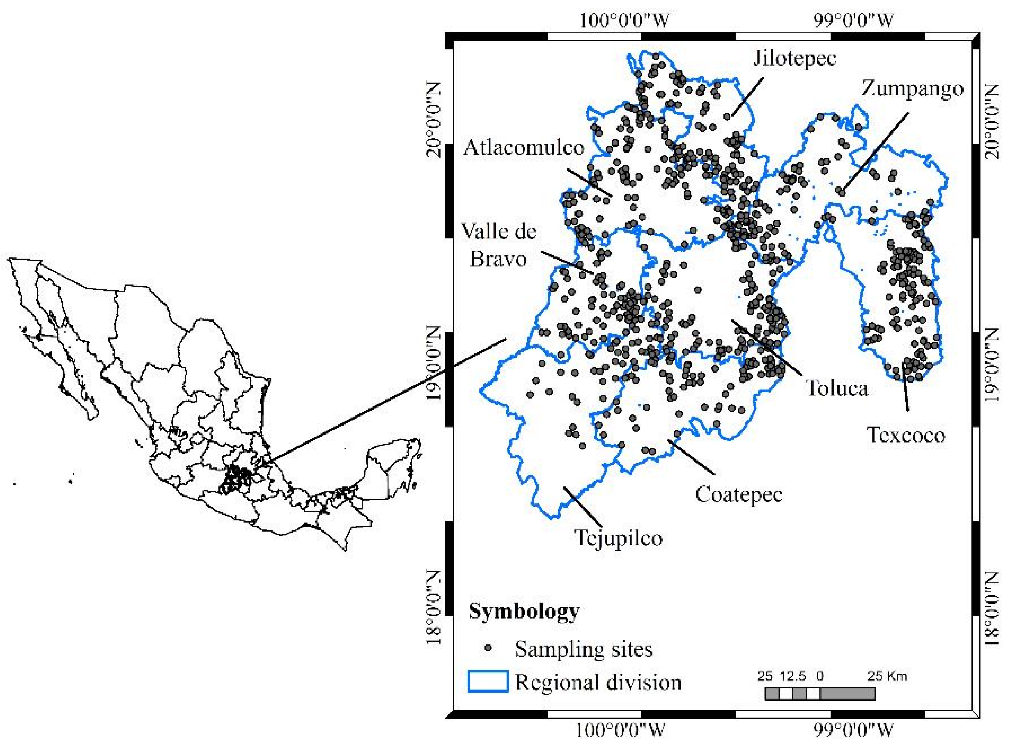
The study was carried out from January to September 2015; 754 circular sampling sites of 1000 m
2 were established and distributed in eight forest regions of the State of Mexico (
Figure 1) [
29].
In each region, we collected information on the type of vegetation cover and land use. The classification of vegetation was established according to the land use and vegetation chart, Series IV, scale 1:250,000 [
30], and was verified in the field.
2.1. Spatial Projection to Evaluate Sampling Designs
The regional survey was planned as a complement to the National Forest and Soil Inventory (NFSI) in a simplified way, where the height and crown diameters were not measured as done in the NFSI. These variables were planned to be estimated from the state and national surveys.
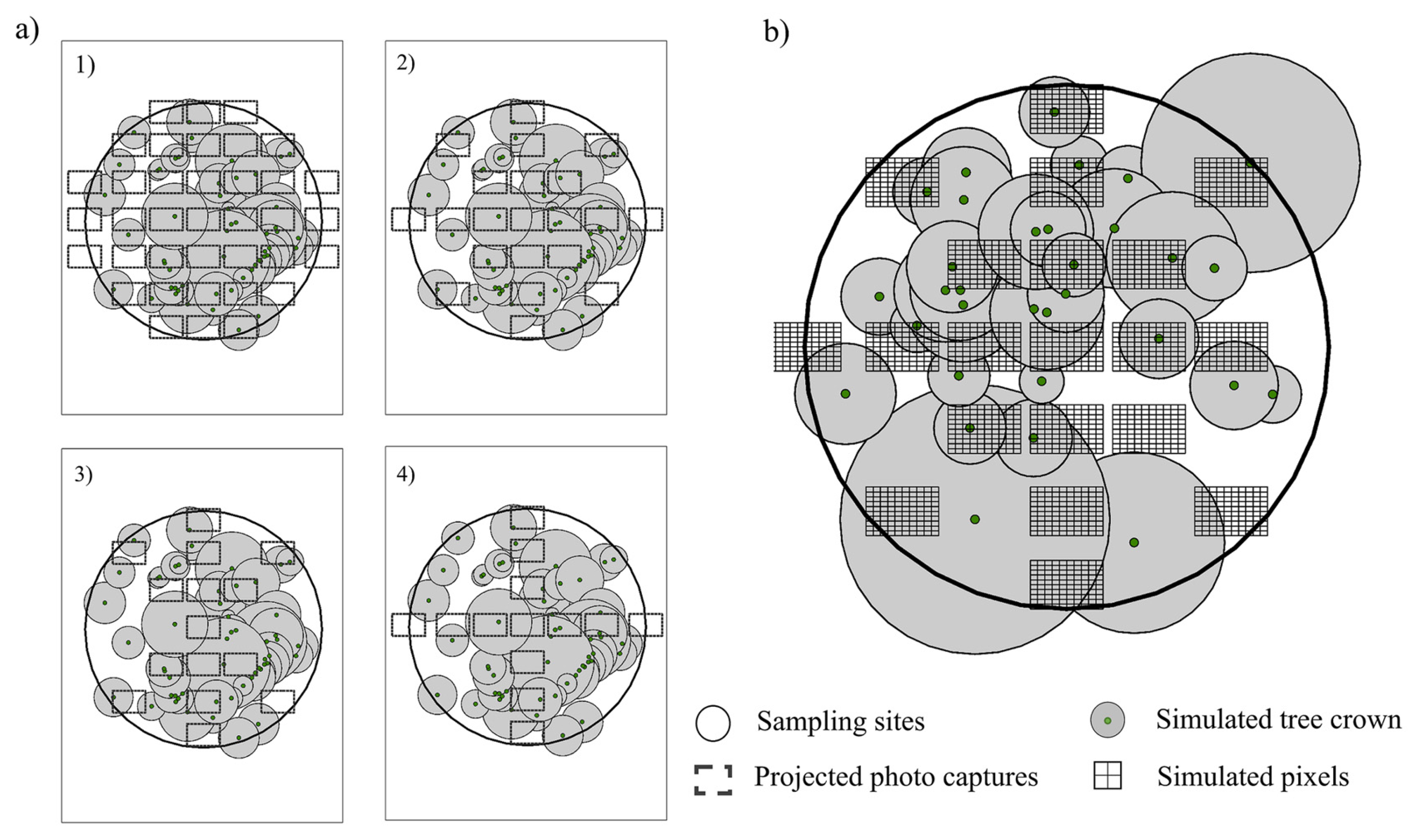
Before the survey phase, a pre-survey of 30 sites was carried out in the Texcoco forest region to evaluate the spatial pattern of trees in four sampling designs of vegetation cover. Comparisons were made between VALERI [
31] and SLAT [
32] designs, along with two alternative samples: CBSP (carbon and biomass sampling plots) and RM (regular mesh). The VALERI design is composed of 13 samples, SLAT of 15 samples, CBSP of 21 samples, and RM of 37 samples (
Figure 2a).
Due to the difficulties of knowing the real vegetation cover within a sampling site, the comparison of sampling designs was performed within a geographic information system. Initially, we recorded the central coordinates of each site (as planned in the regional survey), the distance of the trees to the central point, and their azimuth. Then we calculated the location of trees using the central location of the plot and the azimuth and distance to the central point of the respective tree.
Given that no sampling of the tree crowns diameter was recorded in the survey, an allometric relationship was established between the crown diameter and diameter at breast height [
25]. The data of this function were obtained from the National Forest and Soil Inventory [
33]. The function is the following: DC = 0.1553 + 0.1859 (Dn) (
R2 = 0.79,
p < 0.001), where DC is the tree crown diameter and Dn is the diameter at breast height. The linear model is generalized because it comprised all of the timber species found in the survey. The estimated DC allowed us to construct the crown influence area projection of the trees, assuming a circular shape.
The spatial patterns of the trees were evaluated using the Average Nearest Neighbor (ANN) equation [
34]. If the pattern of the tree distribution is completely random ANN = 1, if ANN < 1 the trees are grouped, and if ANN > 1 the tree mass is regular (dispersed). The ANN analysis was performed within the ArcGIS (10.3, Esri, Redlands, CA, United States).
2.2. Projected Photographic Captures within the GIS
A single photographic capture area of 16.38 m
2 was established to determine the projected cover per site and type of sampling (the procedure for estimating the area is described below). In each area we built a grid (10 × 10) with the purpose of simulating the pixels of a photographic camera (
Figure 2b).
The total observed cover was calculated by dividing the area of overlapping crowns between the sizes of the plot (1000 m
2). On the other hand, the estimated cover resulted from the following equation:
where
NPSi is the number of projected pixels (grid) intersecting with the tree crown area and
NTP is the total number of pixels per sampling design.
As a quantitative measure of the error, the mean absolute error (
MAE) was estimated:
where
O is the observed value of the total projected cover,
E is the estimated value (Equation (1)), and
N is the number of captures per sampling design.
2.3. Field Sampling
Sampling sites were targeted to include vegetation succession and degradation among land uses in Central Mexico [
29]. Information was collected on sites with and without anthropogenic intervention.
2.4. Photo Features
The photographic images were taken at a resolution of 5184 × 3456 pixels in JPG format. We used a Canon EOS Rebeld T5RM camera. The camera lens was adjusted to a range of 18 to 55 mm focal length and an ISO 200 with aperture and exposure in automatic mode.
2.5. Taking Photos at the Sampling Sites
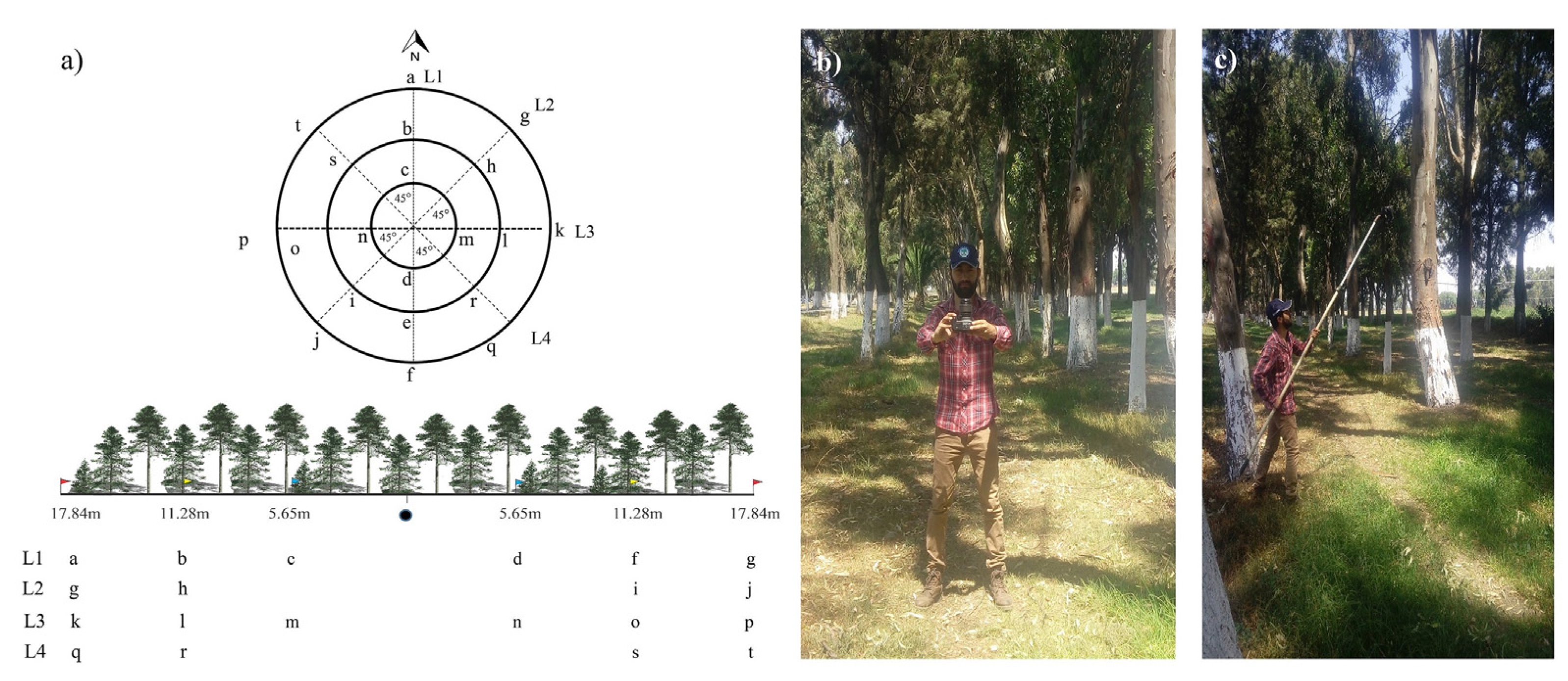
We applied the CBSP sampling design with 21 captures to nadir and zenith, according to
Figure 3a. The lines represent the transects within the sampling site (L1–L4) and each letter represents a photographic capture.
Figure 3b shows the photograph taken at zenith, where the distance between the camera and the ground is 1.5 m.
Figure 3c shows the process of shooting understory (shrub and herbaceous strata), where the interference of the personnel in the photograph was avoided using a stick of five meters long; in this case, the distance between the camera and the ground was 3 m. Two levels of bubble were used to control the angle in which the photographs were taken, one near the operator and the other one stuck to the side of the camera.
The purpose of the CBSP sampling was to capture the largest possible physical area with the fewest samples. To do so, the visual field angle of the lens (
θ) was adjusted depending on the size of the sensor (
n) and its focal length (
f):
The real area covered by a photograph depends on three variables: sensor size (
nij), focal length of the lens (
f), and distance of the lens to the object (
h). In the case of nadir,
h is the distance between the camera lens and the ground. For zenith,
h corresponds to the distance between the lens and the tree crowns. Equation (4) defines the calculation of the real area of the photograph:
where
G is the actual length of the object in the horizontal (
i) and vertical (
j), where the horizontal distance of the
ni sensor size of the camera used was 22.3 mm and the vertical distance
nj was 14.9 mm.
The value of f for the nadir photographs was set at 18 mm because h was established at 3 m. By solving Equation (4), we estimated a real area to nadir of 9.2 m2.
In the case of zenith photographs, a larger real area was required to be representative at the sampling site. The minimum average height of the tree crowns in the forested areas of the region was 4 m. At this point, the value of θ must be adjusted to reach the largest surface, so the value of f was set at 18 mm. Then, by solving Equation (4), the real area at zenith is 16.38 m2.
In heterogeneous forests, such as the study area, the height of the trees can vary in short distances, so in order to maintain the area captured independently of the height of the tree, the value of f can be adjusted by multiplying the average height of the trees at the point of capture by the constant 4.5 (f = 4.5 × h). If the height value was four meters, the camera was placed as close as possible to the ground; in the case of exceeding six meters in height, the camera was placed at a fixed distance of 1.5 m on the ground.
2.6. Estimation of over and Understory Cover
The processing of images to estimate the vegetation cover is different in nadir and zenith projections; in the first case a robust classifier is needed to distinguish the shade of the vegetation, whereas the second one requires a methodology that distinguishes the cover of the canopy in contrast to the sky (atmosphere). Due to the large number of photographs that needed to be processed (24,182 photographs), a code was written in the Python 2.7RM language (Python Software Foundation (PSF): Wilmington, DE, USA) to optimize the process (the software can be requested from the authors). The following sections describe the methodology used.
2.6.1. Estimation of Overstory Cover
The photographs were taken in the morning and in the afternoon, before the sun surpassed 130° of azimuth or after 230° to avoid confusion due to the brightness of the leaves in association with the sky. We used the SunEarthTool tool (
http://www.sunearthtools.com/dp/tools/pos_sun.php) to identify the appropriate times to take the photographs.
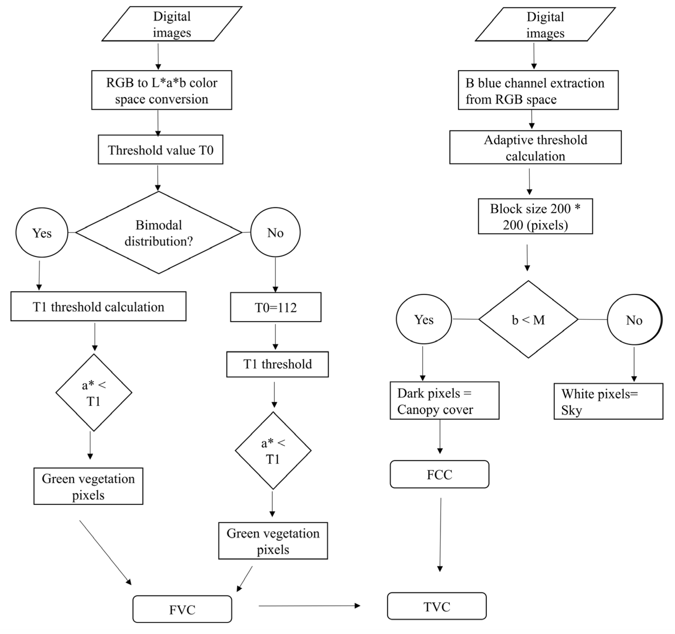
The methodology of Fuentes et al. [
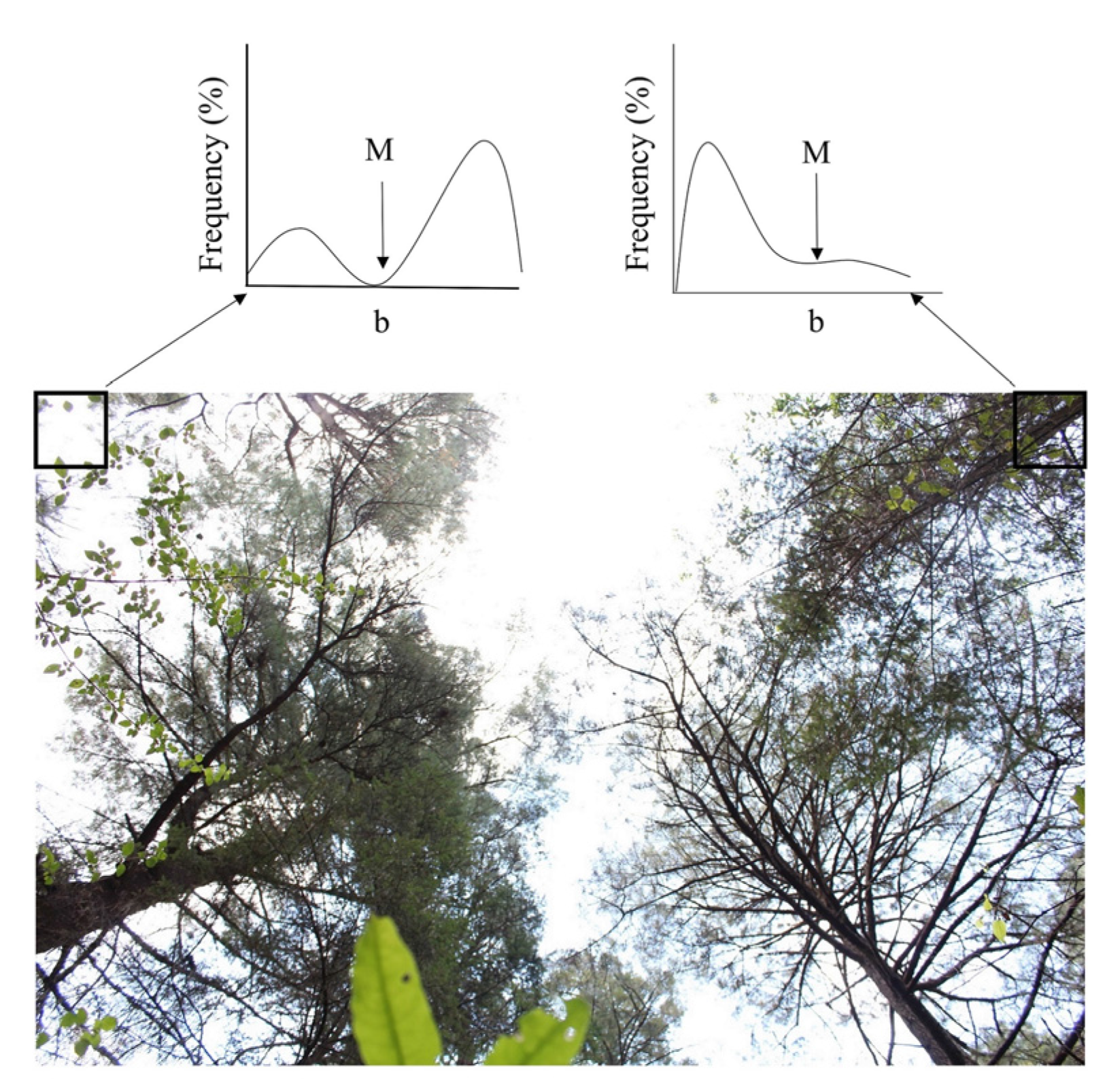
15] was adjusted within the Python language for image processing. The images were converted to vector format in order to separate the three color channels (R, G, B). The blue channel (B) was used to filter the clouds from the image because it gives the best contrast between the cover of the foliage and the sky with the presence of clouds. The adaptive threshold method was used to classify the image [
35].
The method consists of dividing the image into sub-images. The threshold (M) of the sub-image is calculated using the mean or median Gaussian methods. In this case, the median was used as a threshold to perform the separation. The size of the blocks used to divide the image was 200 × 200 pixels. The sum of the proportions of the number of pixels with vegetation in each block to the total number of pixels of the photograph was the cover of the canopy per photograph.
Figure 4 shows an outline of the threshold calculation using this method. The overstory cover includes branches and the upper stems of trees.
2.6.2. Estimation of Understory Cover
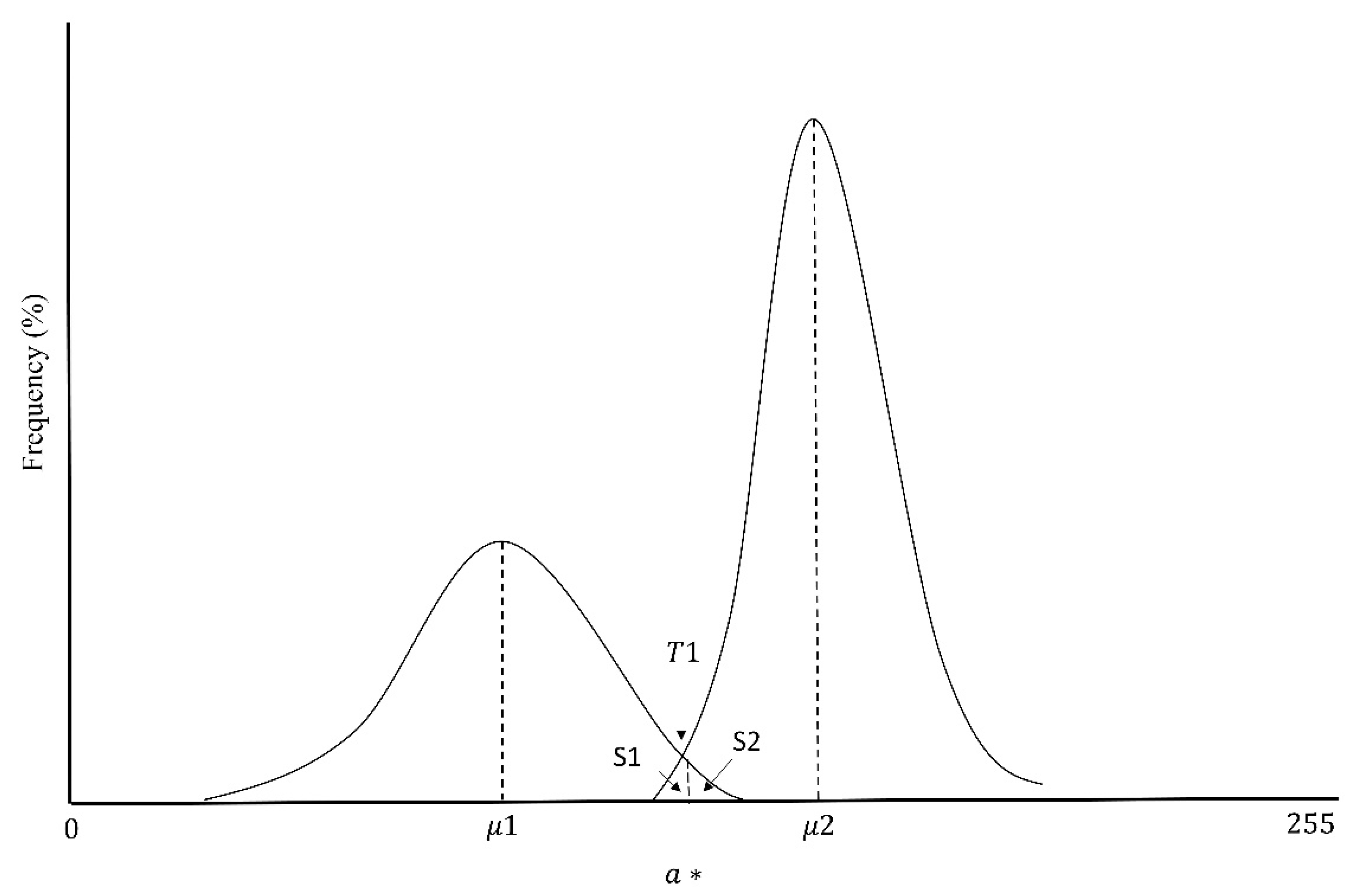
The classification of green vegetation and soil was achieved by calculating a threshold within a two-dimensional space. The images were transformed in the color space L*a*b* [
10]. The green-red component a* was used to distinguish the vegetation from the bare soil, where the values skewed to the left of the histogram indicated green pixels (vegetation) and those skewed to the right showed pixels in red (bare soil). The assumption of the methodology is that the distribution of this component tends to be a bimodal Gaussian distribution.
where
μ1 and
μ2 are the green vegetation and soil average, respectively; and
σ1 and
σ2 are the standard deviations of green vegetation and soil, respectively. The value
W1 is a weighting of the pixels in green and
W2 is the respective weighting for soil. The image is scaled to values of 0–255.
Threshold Adjustment
Regardless of the land use, the value of the pixels is between 75 and 150 in all photographs; to make an optimal adjustment, an initial threshold was set, which was obtained in the middle of the range 75–150 (
T0 = 112). The optimal value of the threshold (
T1) occurred when the functions of Equation (5) were equal (
Figure 5). In this case, the error of omission of vegetation and soil classification, represented by areas S1 and S2, is minimal. The following equation was used to solve
T1:
where:
In extreme situations where bimodality is not evident, that is, photographs where there is only vegetation or bare soil, we applied the algorithm proposed by Liu et al. [
10].
2.6.3. Calculation of Total Vegetation Cover
Total vegetation cover (
TVC) was calculated as follows (
Figure 6):
where
FCC is the proportion of the number of pixels classified as aerial (overstory) cover,
FCV is the fraction of the vegetative cover of the understory (lower stratum), and
NPT is the total number of pixels contained in the image. The sum of
TVC in all images of the CBSP design was considered the total cover per plot.
Figure 6 presents the flowchart of the process of classification.
2.6.4. Accuracy in Cover Classification
The accuracy of the cover estimates obtained using the proposed methodology was calculated through a comparison of these values using a visual classification of the images within the ENVI 5.0
RM program. We considered two classes to distinguish the colors in the photographs. In understory, all pixels in green were considered as leaves, and the rest were classified as bare soil. In overgrowth, all pixels corresponding to leaves, stems, and branches were classified as cover, and the rest of the pixels were classified as sky. As mentioned in [
11], visual classification is considered as the real values of cover in the image and those are compared with the automated threshold proposed in this research.
Images of 12 zenith plots (252 images) and 11 plots to nadir (231 images) were used. The plots represented different land uses. The accuracy of the implemented classifier (
AC) was evaluated using the following formula [
11].
where
A represents the number of pixels with a real presence of vegetation in the reference image (visual classification) and
B represents the number of pixels classified as having vegetation in the applied methods. An average accuracy was obtained in each plot evaluated, where 100% corresponds to a classification without errors.
3. Results
3.1. Sampling Design
The observed (total area of projected crowns) and estimated (projected photographic captured area) values of the projected cover (%) per type of sampling design and spatial pattern of the trees are shown in
Table 1. In the pattern analysis of the trees, 10 plots corresponded to a grouped (clustered) pattern, 15 to a random pattern, and five plots belonged to a dispersed cluster. The calculation of the estimated area is explained in Equation (1).
The CBSP design showed the least error in two of the three types of spatial patterns. The second design that showed minor error was SLAT, which indicates that the sampling design with photographic captures in diagonal form exhibits better results. The RM and VALERI designs had the highest and lowest number of samples, respectively. However, their errors were the highest (MAE > 0.15). These results practically discard them from being considered in operational sampling.
The random spatial pattern showed a higher coefficient of variation (CV) in the four sampling designs due to the design geometry. The dispersed pattern was the second one with the highest CV in the CBSP, SLAT, and VALERI designs. Within the grouped pattern, the CBSP sample recorded the lowest variation.
3.2. Segmentation of Images
The use of the Python program allowed us to make the segmentation threshold selection consistent. The number of captured photos in the sampling makes it impractical to analyze the photographs in a supervised way or in semi-automated processes (photo by photo). The developed program classifies a sampling plot of 42 photographs at zenith and nadir in 30 s. The processor used has 2.6 GHz and 8 GB of memory.
3.3. Classification of Overstory Images
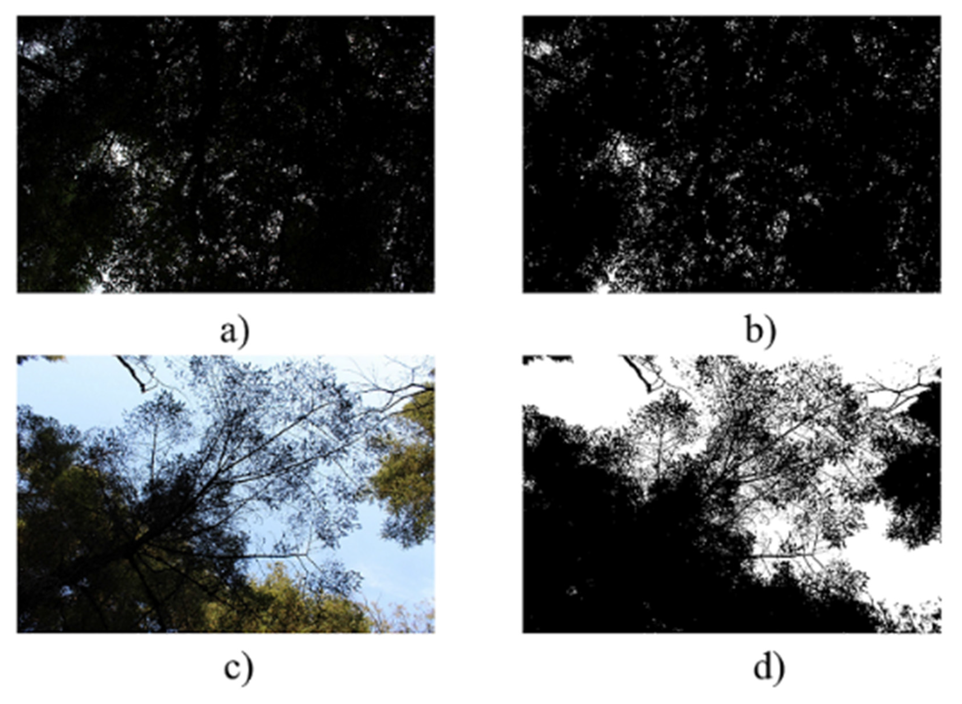
Figure 7 shows the classification of zenith images in four cover conditions.
Figure 7a and its classification 7b represent the photograph with the highest cover in the whole 97% sampling (Oyamel fir forest).
Figure 7c, d represent 50% cover (Oyamel fir forest secondary vegetation).
Figure 7g shows how the classifier correctly discriminates foliage from clouds (secondary vegetation of Pine Forest). Finally,
Figure 7i presents a correct classification with minimum cover (secondary vegetation of Pine Forest).
3.4. Classification of Undestory Images
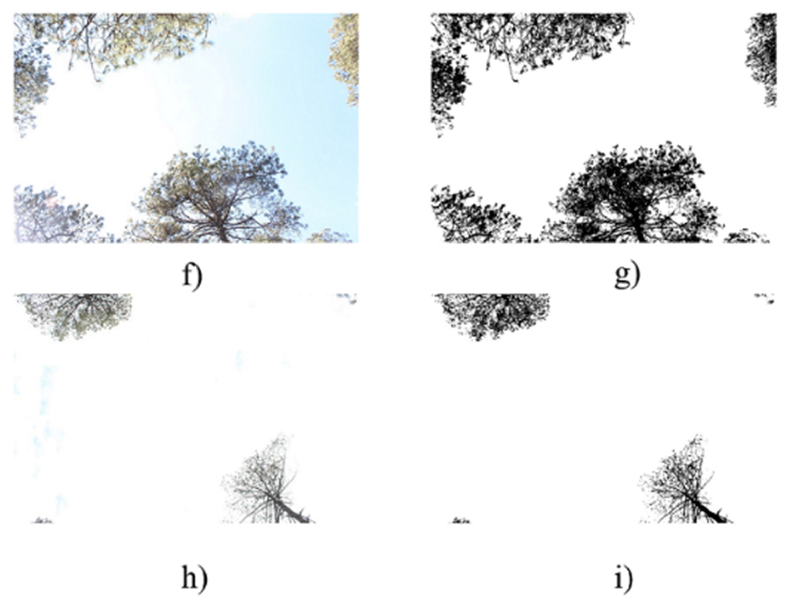
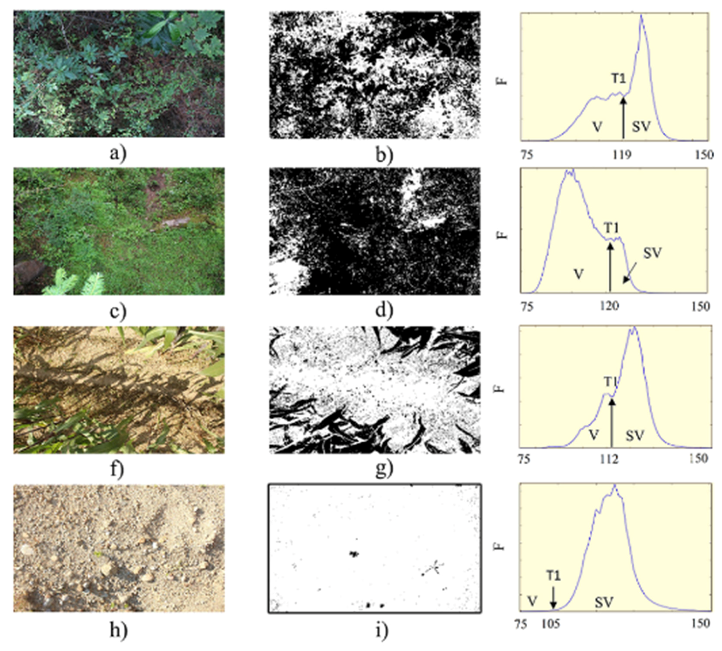
Figure 8 presents a sample of four photographs in different land use and different illumination and vegetation cover conditions, as well as their respective classification and histogram.
Figure 8a,b are presented within a plot of land with secondary vegetation of Oyamel fir forest; the threshold in this capture was a* = 119 and the area under the curve with vegetation (V) was 43%.
Figure 8c,d correspond to herbaceous vegetation within an Oyamel fir forest; in this particular vegetation the illumination was reduced because of the high overstory cover, with an understory cover of 62%.
Figure 8f,g show the image within a Rainfed Agriculture area and we observed that the classifier adequately discriminated between bare soil vegetation and shadows; the threshold in this image was a* = 122 and the vegetation cover was 35%.
Figure 8i,h are presented within a plot without vegetation; the classifier was able to detect the minimal green cover found in the photograph. In this case, as the distribution of the histogram was unimodal, the threshold was set at a* < 105 and the vegetation cover was 0.8%.
3.5. Accuracy of the Classification
Table 2 presents the comparison of the classified cover (%) by the supervised classification method (visual classification) and the zenith method (Estimated). The accuracy was high in all land uses with an average of 93%. In relation to the coefficient of variation CV (representing the variability of the sampling design), we observed that this variability increased as the estimated cover of the different land uses declined. In primary forests (BQP, BQ, BA, BPQ), the variation of the sampling design was low; insofar as there was disturbance in the land use (VSa, VSA, VSh) the variation increased because the static designs were sensitive to the opening of the canopy.
Table 3 presents the evaluation of the vegetative cover to nadir. The average accuracy was 94%. As in zenith, the estimated cover maintains a negative correlation with CV. For this classification, the greatest cover is found in secondary herbaceous vegetation (VSh) where the variability of the sampling is lower; as the vegetation transits to mature forest, the CV is high due to the fact that the understory cover is random. In sites with non-vascular vegetation (bryophytes), the classifier overestimates the percentage of vascular vegetation because it associates the green color with this type of cover.
4. Application of CBSP Design to the Regional Survey
After validating that the CBSP design was robust and precise enough to be used in a regional survey, it was implemented in the campaign through a replication of the procedure used in the pre-survey evaluation in the 754 sampling plots.
It is identified that the application of the sampling design allowed us to capture photographs in an easy and fast way in the majority of land uses.
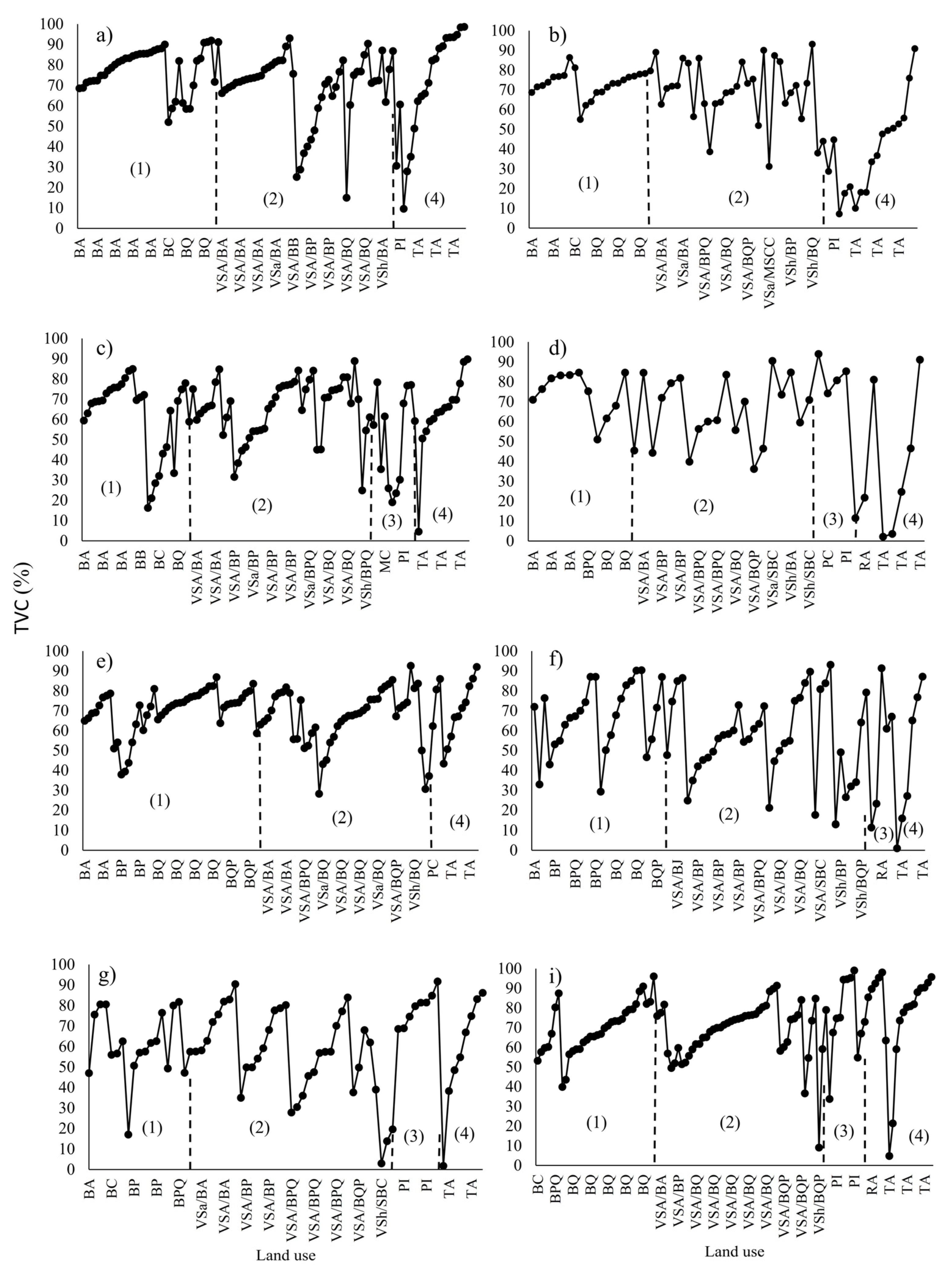
Figure 9 shows the average total vegetation cover of the main land uses in the regions of the State of Mexico. The cover data are presented from highest to lowest and from mature forest to agriculture. Mature forests have a tendency of 50–90% cover in the eight regions, and there was higher average coverage in the region of Toluca (70–90%) (
Figure 9a); in wooded areas with secondary tree vegetation (VSA) and secondary shrub and herbaceous vegetation (VSa and Vsh), the cover ranges from 20 to 90%. This is because the limit of tree vegetation in these plots is a mixture of perennial and deciduous cover, therefore presenting a seasonal change of vegetation cover because of the weather pattern. In this case, the region with the highest coverage was Zumpango (
Figure 9b) and that with the lowest coverage was Coatepec (
Figure 9f).
With regard to cover in agricultural areas (RA, TA), the development of cover over time follows a spatial pattern associated with the time of planting and growth. Cover starts at <10% in all regions and the percentage increases up to 100%, as in the Toluca and Texcoco regions (
Figure 9a,c).
5. Discussion
The use of digital photography for vegetation cover estimations is an easy, low-cost, and potentially suitable approach for hard-to-reach places. These properties give this method an advantage over direct (destructive) and indirect (fisheye cameras) methods [
13]. In Mexico, operational surveys such as the National Forest and Soils Survey [
33] generate vegetation cover estimations that rely on the technician criteria in the field. This research proposes an accurate survey design method which is potentially suitable for the forest sector in the country.
The advantage of using field data is its strength for the validation of satellite information, as a way to use the cover values at greater scales [
6]. On the other hand, a disadvantage of field photography data is the requirement of several photographs in order to produce a reliable estimate. However, there are software methods for the automation of these processes, such as the one proposed in this research.
5.1. Sampling Designs Comparison
One important consideration in field vegetation cover measurements is the need to determine an appropriate sampling design [
31]. The methodologies for measuring vegetation cover are ambiguous in reference to which method should be used to ensure a correct estimation within a sampling plot. The projection made in the GIS allowed us to observe differences in vegetation cover estimations with a simple scheme. The results provide important information for choosing a sampling design and reducing the costs of the collection and processing of field data [
22], considering the large amount of samples of this survey.
Martens et al. [
36] show that the spatial patterns influence the height, cover, and distribution of vegetation in their different strata. Our results showed that, independently of the spatial pattern of the survey sites, sampling designs that captured diagonal photographs (CBSP and SLAT) exhibited the least estimation error.
The advantages of these designs are the low number of photographs needed (42 phothographs) and their easy field implementation. This ratifies the vegetation cover estimation operability using this method and how it can be related to grouping indices to evaluate the effect of the forest management of zones without disturbance on disturbed zones [
24].
5.2. Sampling Survey
Forest surveys in several parts of the world, including Mexico, are carried out in circular plots of 1000 m
2 (17.85 m radius) [
22]. In this research, we adopted this design to evaluate the biomass and carbon storage in different land uses within the State of Mexico. The CBSP design proved to be feasible for its implementation in different land uses and spatial patterns of the trees; this simple design allowed the application in distant sampling points and rugged terrain, which makes it an operative method to capture vegetation cover with digital photographs.
An example of the sampling operability is that bubble levels were used to stabilize the camera at each sampling point, instead of using tripods to fix it. This technique helped to reduce the time to take the photographs and presented no considerable error when compared to tripod shots [
37].
The number of samples and their arrangement was another variable to be considered for the sampling to be operative and related to other variables measured in the plot (i.e., biomass, carbon), so captures were fixed at the ends of the sites [
20]. The CBSP design obtained the best results when estimating the vegetation cover. The efficiency of its application and smaller errors in the cover estimation turns it into a practical design for this type of application, besides saving storage and time when processing the images.
The spatial distribution of trees within the site is an important element for the dynamics of the forest ecosystem [
26]. In the case of overstory cover, we observed that the applied sampling design showed a negative trend between the estimated cover and its coefficient of variation (CV). The primary forests presented high and compact canopy covers (low CV); when reducing it, the canopy cover tends to be dispersed (high CV). In the case of understory cover, the opposite occurs. In disturbed areas (secondary vegetation), the cover is larger and compact; when this cover is reduced, the pattern is dispersed.
The real area of a photograph is another important aspect that has been little explored in vegetation cover sampling design. Researchers generally use a fixed lens viewing angle (35–40°) to estimate the canopy cover, so a greater opening angle would be measuring the closure of the canopy. Jennings et al. [
38] describe in detail the difference between these two concepts. In this study, we observed that in real situations the height of the trees in a sampling site is heterogeneous. For this reason, we proposed to adjust the focal length of the camera at the point of capture by a constant as this ensures that one is able to approximate and make repeatable the capture area independently of the architecture of the trees.
5.3. Automated Classification of Images
The automation of vegetative cover classification is a process that avoids the error of the human component and ensures the possibility of reproducing the results [
11]. The efforts to automate image classification have focused on programs such as MATLAB [
12,
15,
39], WinScanopy [
40], or Photoshop [
41], among others. But although the former meets the requirement of making the batch processing of the images operative, it has the disadvantage of having an additional cost. The other programs have the disadvantage of processing the images photo by photo, which discarded them for the analysis of cover in this study. The Python
RM program was chosen for the versatility of the specialized libraries available, and for being a free access program. The written code enabled us to process in batch the images of the sampling in a time similar to that described in programs like MATLAB.
5.3.1. Overstory Cover
In the classification of digital photographs, binary methods (global thresholds) are generally used to estimate canopy cover [
42]. The colors of the classified images have gray tonalities for vegetation and white for the sky. According to Chityala and Pudipeddi [
35], the accuracy in the classification for the global threshold methods is low. The problem is trying to find the maximum variance between two logical groups of segments within the whole image, which can cause confusion in the classification by overexposure in the camera or image capture at inappropriate times. In this research, we propose the use of the adaptive threshold in the blue space of the image [
15]. The method is based on the same principles of the global threshold, but the segmentation statistics are done at the block level within the image, allowing greater accuracy in the overall classification.
The accuracy of the classification is high and related to the comparison of binary algorithms performed by Ghatthorn and Beckschäfer [
42]. The sampling was directed to avoid the effect of the sun (the captures were made before noon and at near sunset); however, in the sampling, there were circumstances that caused the photographs to exceed the proposed range, such as the VSh/BPQ land use plot (
Table 2), which showed the lowest precision (87%) [
16]. Nonetheless, the development of methodologies applied to this problem are beyond the scope of this research.
5.3.2. Understory Cover
There are many methods to extract the vegetation cover fraction [
11,
12,
43] so the degree of accuracy is an important factor in the efficiency of field measurements. For example, supervised classification has a high accuracy but low efficiency, while unsupervised classification has a high efficiency but low precision due to commission and omission errors [
1].
The algorithm proposed by Liu et al. [
10] has the property of being simple, easy to automate, and has a high degree of precision. When comparing it with the supervised classification in different sampling plots, the results in terms of precision were high (>87%); the main problem of the misclassification was the confusion of the vascular vegetation with bryophytes, which in the color space *a detects a green color that is difficult to discern. In conditions of low illumination due to the effect of the canopy, the algorithm had no problems in correctly classifying vegetation and shade [
12], and with a single component predomination (bare soil) in the photograph, the classifier generated good results (
Figure 8i).
The two methods proposed to evaluate the over and understory vegetation cover were robust and replicable in all sampling plots. The reason for estimating the foliar projective cover rather than the leaf area index is that the former is a more adequate variable to characterize vegetation [
44] since the projective foliar cover captured with digital photographs contains information on individual plants and their spatial distribution. With this perspective and considering the validation of the proposed sampling and plot area, we will contemplate the validation of biophysical variables calculated with remote sensors in future work of the research group.
6. Conclusions
The over and understory vegetation cover was estimated with digital photographs in sampling plots of the State of Mexico. The high efficiency and precision of the classification methods indicate that they are robust for discerning vegetation in different land uses and illumination conditions.
The use of digital photography reduces the ambiguity of vegetation cover estimations in regional and national surveys. The proposed method is easily reproducible in heterogeneous land and vegetation conditions.
The automation of the process using a free programming language avoided human errors and ensured the reproducibility of the results at a low cost.
The sampling methods using the capture of diagonal-angled photographs were the best way to obtain less biased information when taking digital photographs at a circular sampling site. The simulation showed that the CBSP design has a smaller error when considering the spatial distribution of trees within the sampling site. Its easy field management, the number of photographs per site, and its precision make it an operative design. One additional advantage of the proposed field survey is that the real area covered by the photograph is independent of the height of trees. This guarantees representability and avoids image superposition in the sampling site.
Mature forests have a high and compact overstory vegetation cover, which tends to be reduced in secondary forests. The greater cover of the understory is found in secondary forests, where it is denser. The cover of the undergrowth declines in mature forests.
The application of this method for regional and national surveys is recommended.


