Countering Negative Effects of Terrain Slope on Airborne Laser Scanner Data Using Procrustean Transformation and Histogram Matching

 , ,
, ,
Abstract
:1. Introduction
2. Materials and Methods
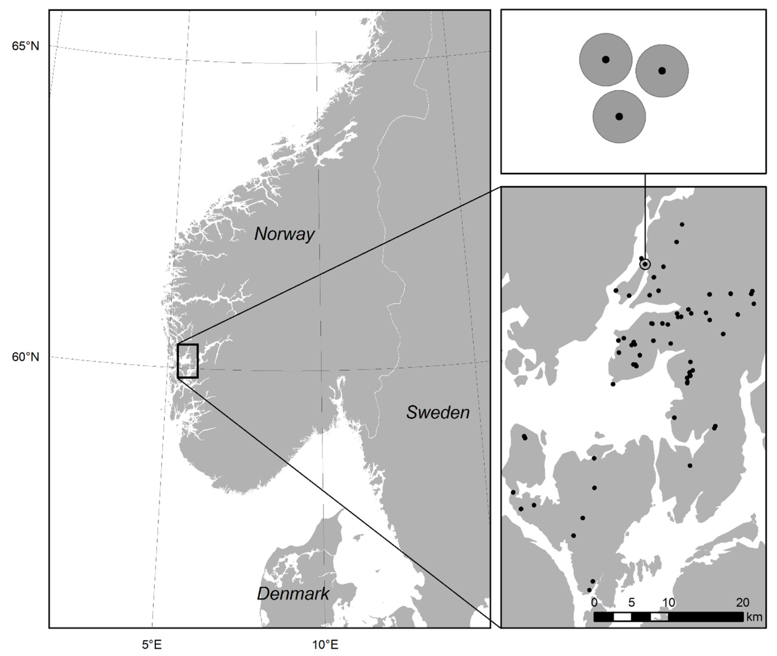
2.1. Study Area
2.2. Field Data
2.3. ALS Data and Initial Processing
2.4. Transformations
- (1)
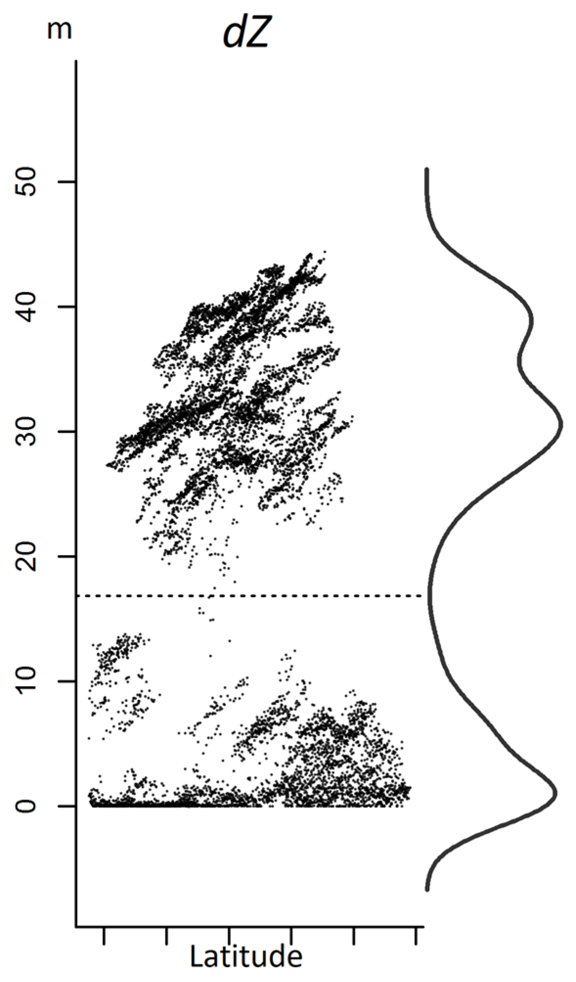
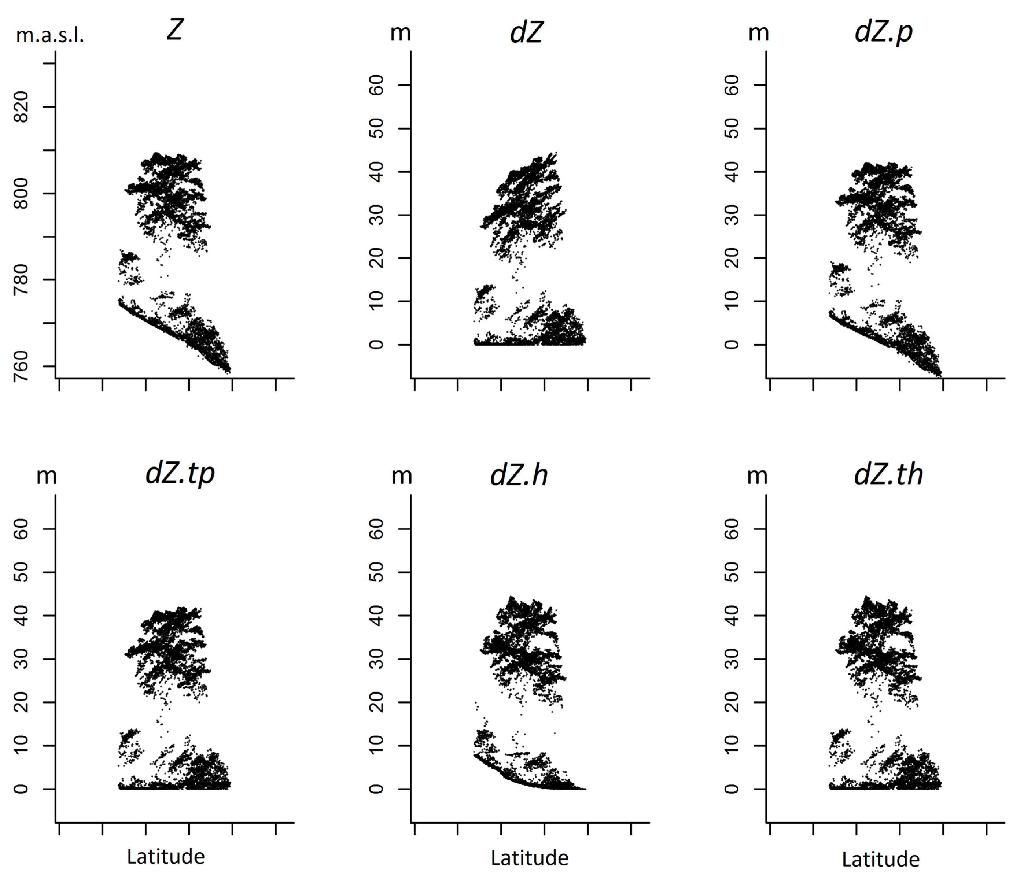
- the normalized point cloud (dZ),
- (2)
- the normalized point cloud with PT (dZ.p),
- (3)
- the normalized point cloud with PT above a threshold (dZ.tp),
- (4)
- the normalized point cloud with HM (dZ.h), and
- (5)
- the normalized point cloud with HM above a threshold (dZ.th).
2.4.1. PT
2.4.2. HM
2.5. ALS Metrics
2.6. Generalized Linear Modeling
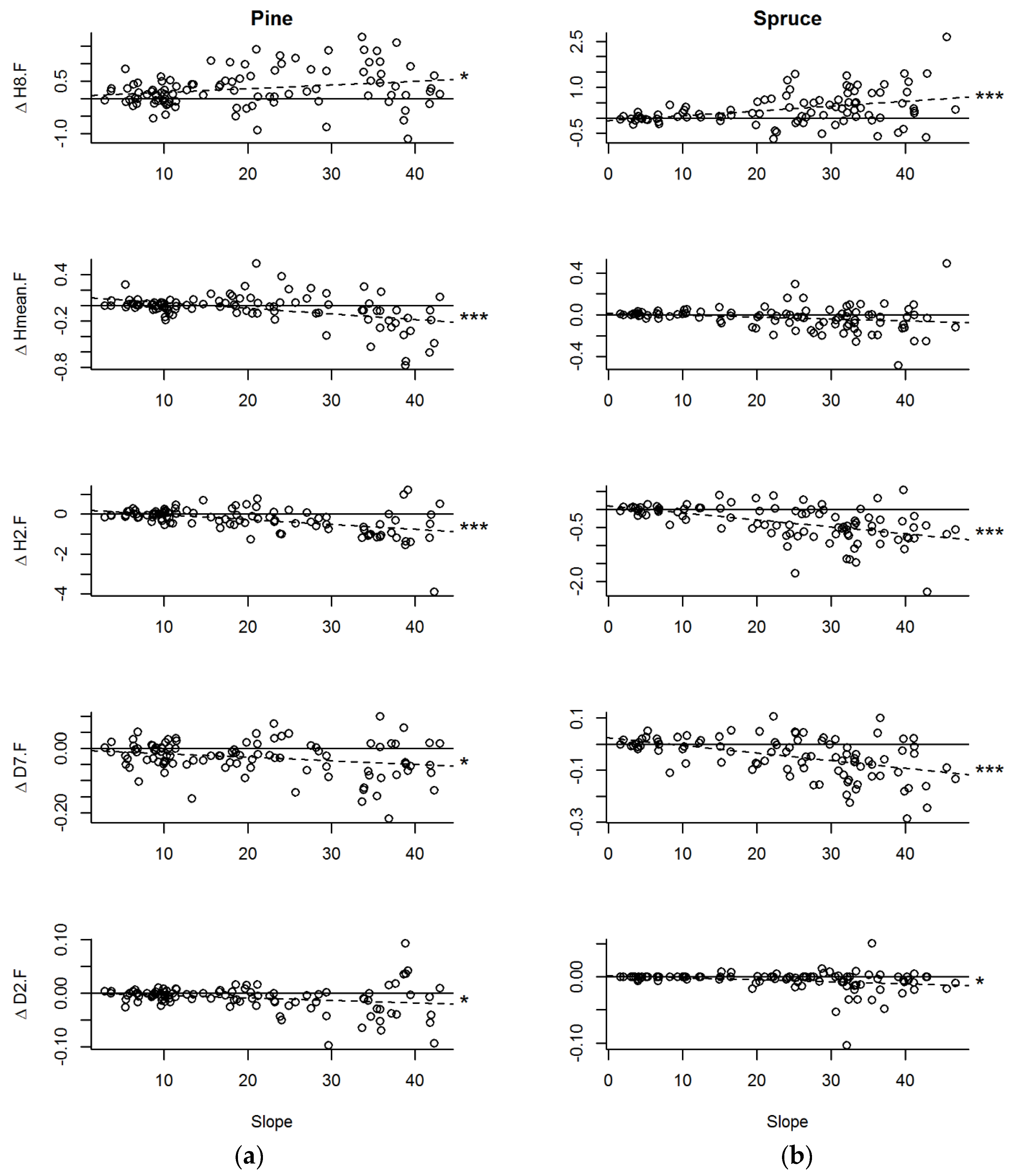
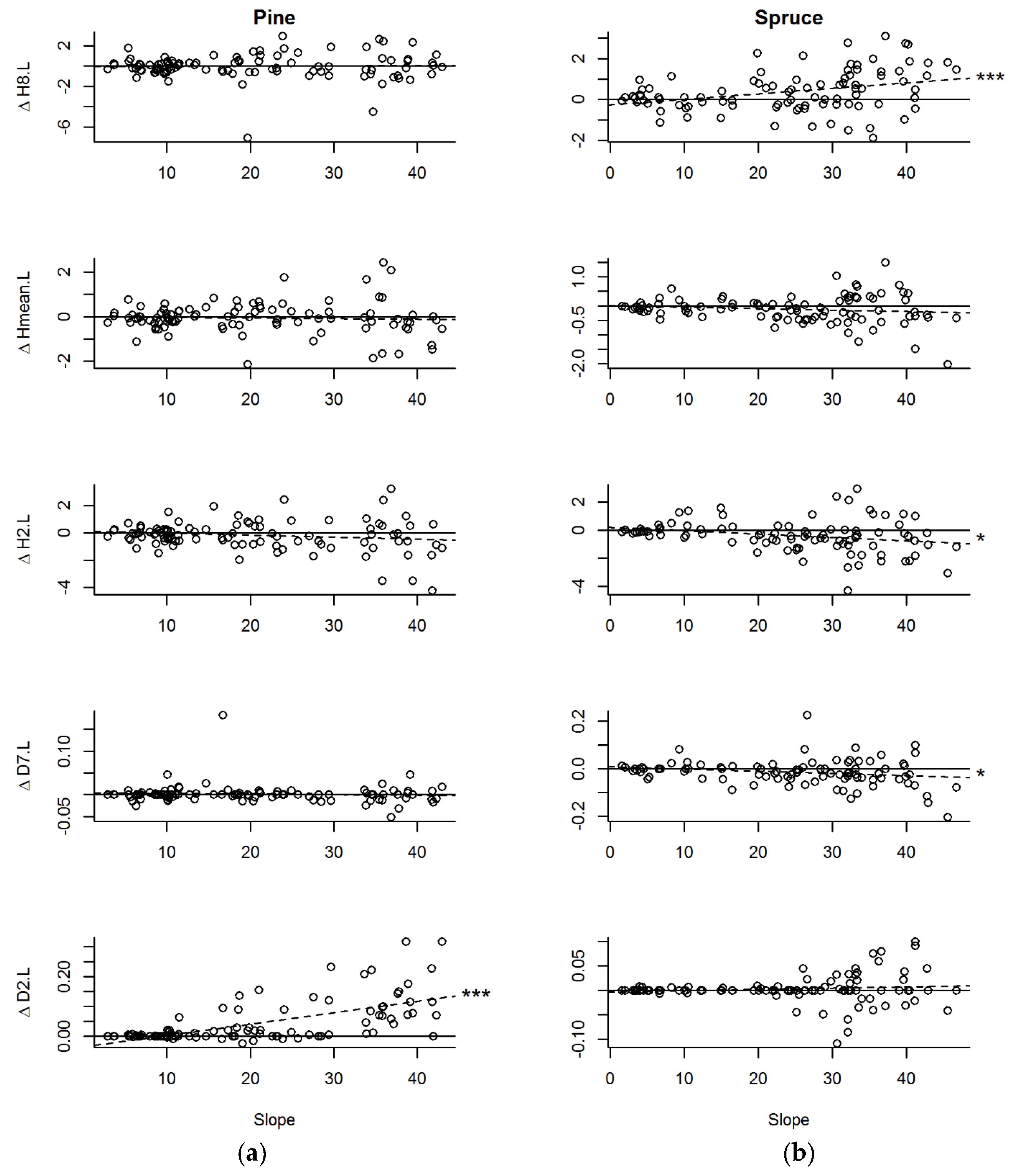
2.7. Summarizing Modeling Results
3. Results
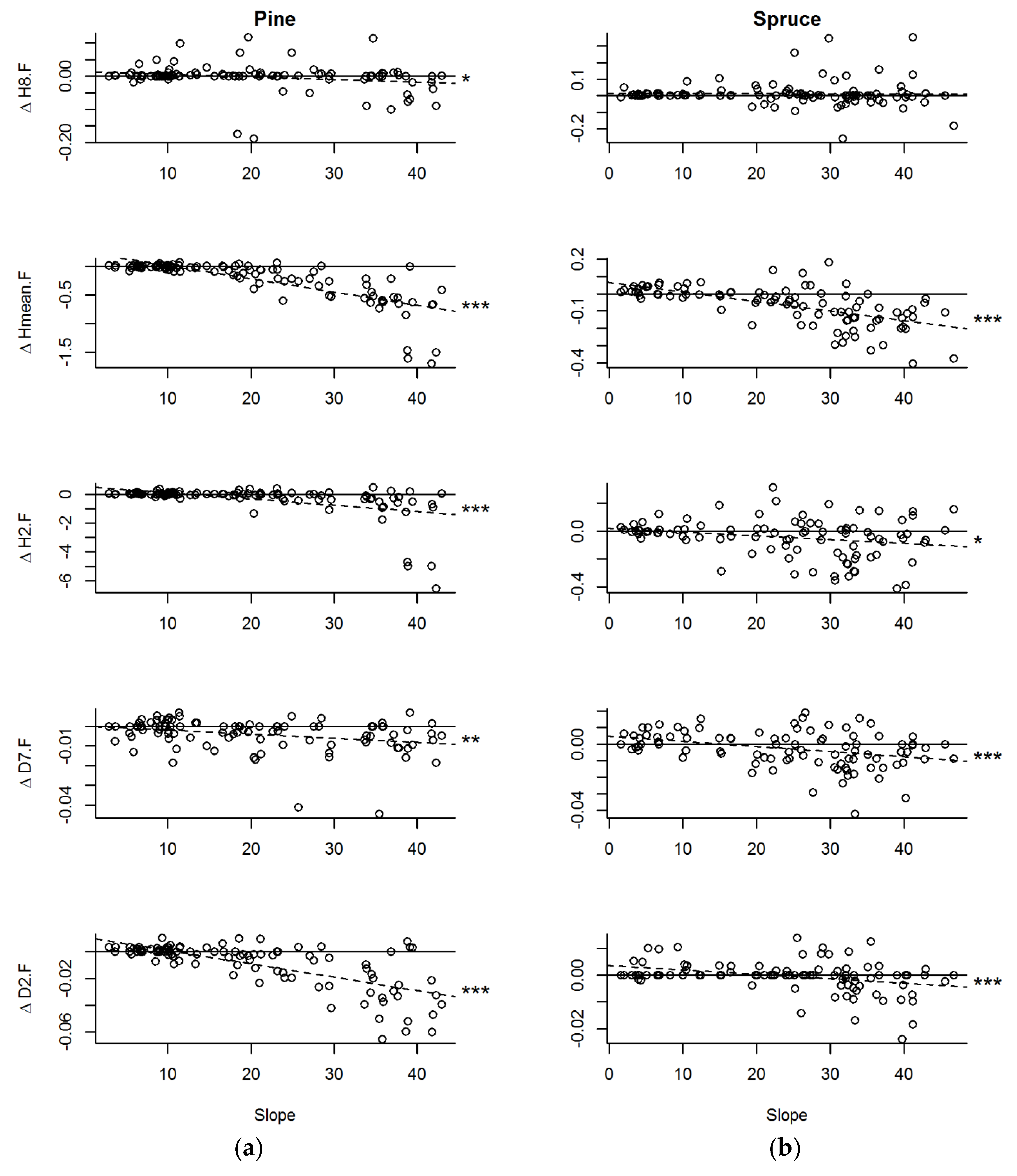
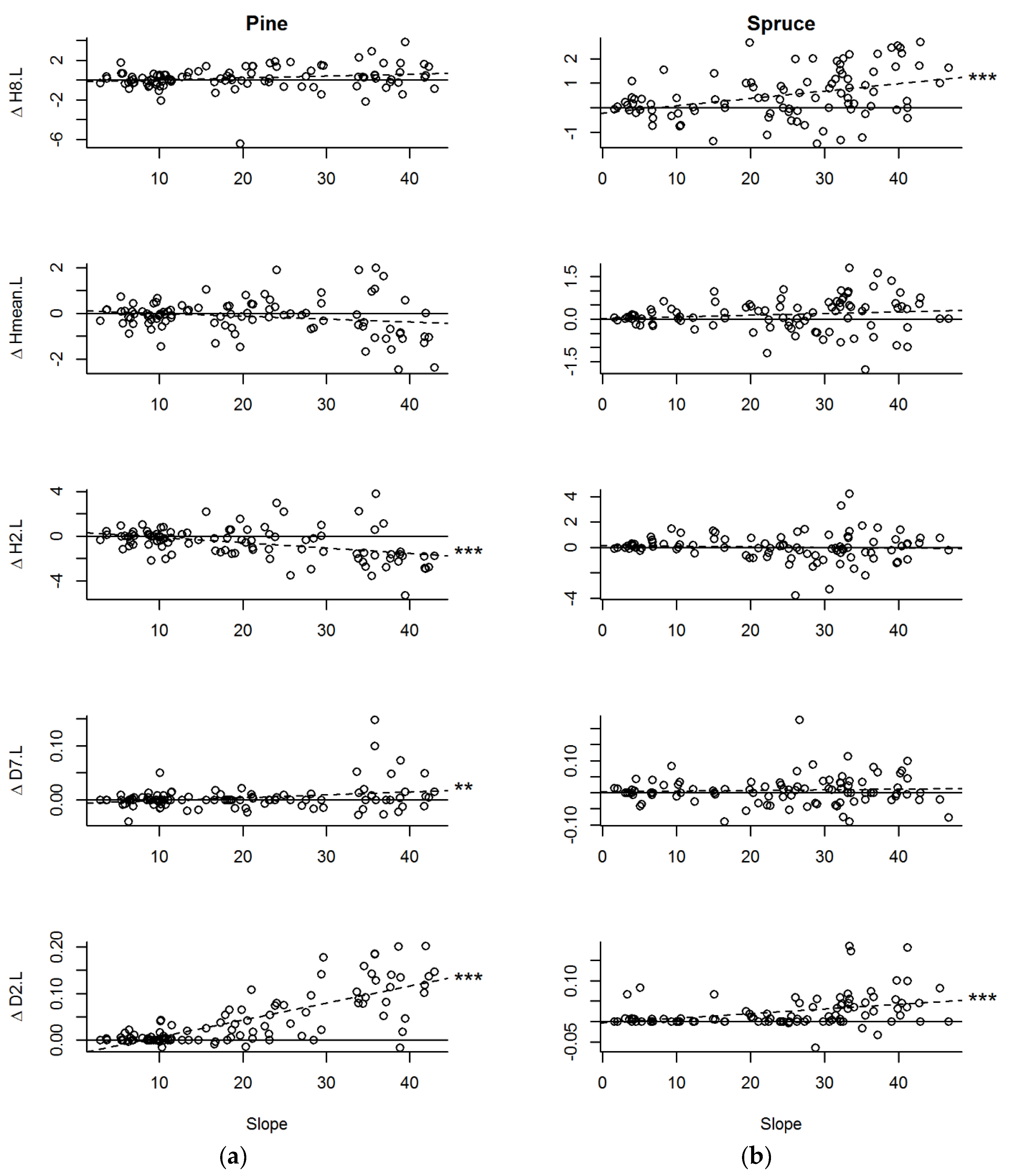
3.1. ALS Metrics
3.2. Regression Models
3.3. Summarizing Modeling Results
4. Discussion
5. Conclusions
Acknowledgments
Author Contributions
Conflicts of Interest
References
- White, J.C.; Coops, N.C.; Wulder, M.A.; Vastaranta, M.; Hilker, T.; Tompalski, P. Remote sensing technologies for enhancing forest inventories: A review. Can. J. Remote Sens. 2016, 42, 619–642. [Google Scholar] [CrossRef]
- Bollandsås, O.M.; Hanssen, K.H.; Marthiniussen, S.; Næsset, E. Measures of spatial forest structure derived from airborne laser data are associated with natural regeneration patterns in an uneven-aged spruce forest. For. Ecol. Manag. 2008, 255, 953–961. [Google Scholar] [CrossRef]
- Breidenbach, J.; Astrup, R. The Semi-Individual Tree Crown Approach. In Forestry Applications of Airborne Laser Scanning; Maltamo, M., Næsset, E., Vauhkonen, J., Eds.; Springer Science Business Media: Dordrecht, The Netherlands, 2014; pp. 113–133. [Google Scholar]
- Breidenbach, J.; Koch, B.; Kändler, G.; Kleusberg, A. Quantifying the influence of slope, aspect, crown shape and stem density on the estimation of tree height at plot level using lidar and InSAR data. Int. J. Remote Sens. 2008, 29, 1511–1536. [Google Scholar] [CrossRef]
- Khosravipour, A.; Skidmore, A.K.; Wang, T.; Isenburg, M.; Khoshelham, K. Effect of slope on treetop detection using a LiDAR Canopy Height Model. ISPRS J. Photogramm. Remote Sens. 2015, 104, 44–52. [Google Scholar] [CrossRef]
- Vega, C.; Hamrouni, A.; El Mokhtari, S.; Morel, J.; Bock, J.; Renaud, J.P.; Bouvier, M.; Durrieu, S. PTrees: A point-based approach to forest tree extraction from lidar data. Int. J. Appl. Earth Obs. Geoinf. 2014, 33, 98–108. [Google Scholar] [CrossRef]
- Graf, R.F.; Mathys, L.; Bollmann, K. Habitat assessment for forest dwelling species using LiDAR remote sensing: Capercaillie in the Alps. For. Ecol. Manag. 2009, 257, 160–167. [Google Scholar] [CrossRef]
- Hill, R.A.; Hinsley, S.A. Airborne lidar for woodland habitat quality monitoring: Exploring the significance of lidar data characteristics when modelling organism-habitat relationships. Remote Sens. 2015, 7, 3446–3466. [Google Scholar] [CrossRef]
- Sverdrup-Thygeson, A.; Ørka, H.O.; Gobakken, T.; Næsset, E. Can airborne laser scanning assist in mapping and monitoring natural forests? For. Ecol. Manag. 2016, 369, 116–125. [Google Scholar] [CrossRef]
- Duan, Z.; Zhao, D.; Zeng, Y.; Zhao, Y.; Wu, B.; Zhu, J. Assessing and Correcting Topographic Effects on Forest Canopy Height Retrieval Using Airborne LiDAR Data. Sensors 2015, 15, 12133–12155. [Google Scholar] [CrossRef] [PubMed]
- Hyyppä, J.; Inkinen, M. Detecting and estimating attributes for single trees using laser scanner. Photogramm. J. Finl. 1999, 16, 27–42. [Google Scholar]
- Næsset, E. Determination of mean tree height of forest stands using airborne laser scanner data. ISPRS J. Photogramm. Remote Sens. 1997, 52, 49–56. [Google Scholar] [CrossRef]
- Næsset, E. Estimating timber volume of forest stands using airborne laser scanner data. Remote Sens. Environ. 1997, 61, 246–253. [Google Scholar] [CrossRef]
- Næsset, E. Area-Based Inventory in Norway—From Innovation to an Operational Reality. In Forestry Applications of Airborne Laser Scanning; Maltamo, M., Næsset, E., Vauhkonen, J., Eds.; Springer Science Business Media: Dordrecht, The Netherlands, 2014; pp. 215–240. [Google Scholar]
- Wulder, M.A.; Coops, N.C.; Hudak, A.T.; Morsdorf, F.; Nelson, R.; Newnham, G.; Vastaranta, M. Status and prospects for LiDAR remote sensing of forested ecosystems. Can. J. Remote Sens. 2013, 39, S1–S5. [Google Scholar] [CrossRef]
- Boas, F. The Horizontal Plane of the Skull and the General Problem of the Comparison of Variable Forms. Science 1905, 21, 862–863. [Google Scholar] [CrossRef] [PubMed]
- Von Neumann, J. Some matrix inequalities and metrization of matrix space. Tomsk Univ. Rev. 1937, 1, 286–300. [Google Scholar]
- Claude, J. Morphometrics with R; Springer: New York, NY, USA, 2008; p. 316. [Google Scholar]
- Slice, D.E. Geometric Morphometrics. Annu. Rev. Anthropol. 2007, 36, 261–281. [Google Scholar] [CrossRef]
- Theobald, D.L. Likelihood and Empirical Bayes Superposition of Multiple Macromolecular Structures. In Bayesian Methods in Structural Bioinformatics; Hamelryck, T., Mardia, K., Ferkinghoff-Borg, J., Eds.; Springer: Berlin/Heidelberg, Germany, 2012; pp. 191–208. [Google Scholar]
- Gonzalez, R.C.; Woods, R.E. Digital Image Processing, 3rd ed.; Prentice-Hall, Inc.: Upper Saddle River, NJ, USA, 2002; p. 793. [Google Scholar]
- Ørka, H.O.; Gobakken, T.; Næsset, E.; Ene, L.; Lien, V. Simultaneously acquired airborne laser scanning and multispectral imagery for individual tree species identification. Can. J. Remote Sens. 2012, 38, 125–138. [Google Scholar] [CrossRef]
- Baffetta, F.; Corona, P.; Fattorini, L. A matching procedure to improve k-NN estimation of forest attribute maps. For. Ecol. Manag. 2012, 272, 35–50. [Google Scholar] [CrossRef] [Green Version]
- Gilichinsky, M.; Heiskanen, J.; Barth, A.; Wallerman, J.; Egberth, M.; Nilsson, M. Histogram matching for the calibration of kNN stem volume estimates. Int. J. Remote Sens. 2012, 33, 7117–7131. [Google Scholar] [CrossRef]
- Vauhkonen, J.; Mehtätalo, L. Matching remotely sensed and field-measured tree size distributions. Can. J. For. Res. 2014, 45, 353–363. [Google Scholar] [CrossRef]
- Xu, Q.; Hou, Z.; Maltamo, M.; Tokola, T. Calibration of area based diameter distribution with individual tree based diameter estimates using airborne laser scanning. ISPRS J. Photogramm. Remote Sens. 2014, 93, 65–75. [Google Scholar] [CrossRef]
- Nyström, M.; Holmgren, J.; Olsson, H. Change detection of mountain birch using multi-temporal ALS point clouds. Remote Sens. Lett. 2013, 4, 190–199. [Google Scholar] [CrossRef]
- Hauglin, M.; Ørka, H. Discriminating between Native Norway Spruce and Invasive Sitka Spruce—A Comparison of Multitemporal Landsat 8 Imagery, Aerial Images and Airborne Laser Scanner Data. Remote Sens. 2016, 8, 363. [Google Scholar] [CrossRef]
- Javad Positioning Systems. Pinnacle User’s Manual; Knowledge Base: San Jose, CA, USA, 1999. [Google Scholar]
- Braastad, H. Volume tables for birch. Rep. Nor. For. Res. Inst. 1966, 21, 265–365. (In Norwegian) [Google Scholar]
- Brantseg, A. Volume functions and tables for Scots pine, South Norway. Rep. Nor. For. Res. Inst. 1967, 22, 689–739. (In Norwegian) [Google Scholar]
- Vestjordet, E. Functions and tables for volume of standing trees, Norway spruce. Rep. Nor. For. Res. Inst. 1967, 22, 543–574. (In Norwegian) [Google Scholar]
- Bauger, E. Tree volume functions and tables. Scots pine, Norway spruce and Sitka spruce in western Norway. Rapp. Skogforsk 1995, 16, 26. (In Norwegian) [Google Scholar]
- Fitje, A.; Vestjordet, E. Stand height curves and new tariff tables for Norway spruce. Rep. Nor. For. Res. Inst. 1977, 34, 23–68. (In Norwegian) [Google Scholar]
- Axelsson, P. DEM generation from laser scanner data using adaptive TIN models. Int. Arch. Photogramm. Remote Sens. 2000, 33, 110–117. [Google Scholar]
- Soininen, A. TerraScan User’s Guide; Helsinki Finland: Terrasolid Oy, Finland, 2016. [Google Scholar]
- Gobakken, T.; Næsset, E.; Nelson, R.; Bollandsås, O.M.; Gregoire, T.G.; Ståhl, G.; Holm, S.; Ørka, H.O.; Astrup, R. Estimating biomass in Hedmark County, Norway using national forest inventory field plots and airborne laser scanning. Remote Sens. Environ. 2012, 123, 443–456. [Google Scholar] [CrossRef]
- Dryden, I.L.; Mardia, K.V. Statistical Shape Analysis: With Applications in R, 2nd ed.; John Wiley and Sons: Hoboken, NJ, USA, 2016; p. 496. ISBN 978-0-470-69962-1. [Google Scholar]
- Borg, I.; Groenen, P.J.F. Modern Multidimensional Scaling: Theory and Applications, 2nd ed.; Springer: New York, NY, USA, 2005; p. 614. ISBN 0-387-25150-2. [Google Scholar]
- R Development Core Team. R: A Language and Environment for Statistical Computing; R Foundation for Statistical Computing: Vienna, Austria, 2016. [Google Scholar]
- Martin, A.D.; Quinn, K.M.; Park, J.H. MCMCpack: Markov Chain Monte Carlo in R. J. Stat. Softw. 2011, 42, 1–21. [Google Scholar] [CrossRef]
- Oksanen, J.; Guillaume Blanchet, F.; Friendly, M.; Kindt, R.; Legendre, P.; McGlinn, D.; Minchin, P.R.; O’Hara, R.B.; Simpson, G.L.; Solymos, P.; et al. Vegan: Community Ecology Package. R Package Version 2.4-2. 2017. Available online: https://CRAN.R-project.org/package=vegan (accessed on 4 October 2017).
- Borchers, H.W. Pracma: Practical Numerical Math Functions. R Package Version 1.9.9. 2017. Available online: https://CRAN.R-project.org/package=pracma (accessed on 4 October 2017).
- Hansen, E.H.; Gobakken, T.; Bollandsås, O.M.; Zahabu, E.; Næsset, E. Modeling Aboveground Biomass in Dense Tropical Submontane Rainforest Using Airborne Laser Scanner Data. Remote Sens. 2015, 7, 788–807. [Google Scholar] [CrossRef] [Green Version]
- Næsset, E.; Gobakken, T. Estimation of above- and below-ground biomass across regions of the boreal forest zone using airborne laser. Remote Sens. Environ. 2008, 112, 3079–3090. [Google Scholar] [CrossRef]
- Næsset, E. Practical large-scale forest stand inventory using a small-footprint airborne scanning laser. Scand. J. For. Res. 2004, 19, 164–179. [Google Scholar] [CrossRef]
- Næsset, E.; Gobakken, T.; Bollandsås, O.M.; Gregoire, T.G.; Nelson, R.; Ståhl, G. Comparison of precision of biomass estimates in regional field sample surveys and airborne LiDAR-assisted surveys in Hedmark County, Norway. Remote Sens. Environ. 2013, 130, 108–120. [Google Scholar] [CrossRef]
- Sugiura, N. Further analysts of the data by Akaike’s information criterion and the finite corrections. Commun. Stat. Theory Methods 1978, 7, 13–26. [Google Scholar] [CrossRef]
- Sestelo, M.; Villanueva, N.M.; Roca-Pardinas, J. Selecting Variables in Regression Models. R package version 2.1.0. 2015. Available online: https://cran.r-project.org/web/packages/FWDselect/index.html (accessed on 1 September 2016).
- Zuur, A.F.; Ieno, E.N.; Walker, N.J.; Saveliev, A.A.; Smith, G.M. Mixed Effects Models in Extensions in Ecology with R. Statistics for Biology and Health; Springer: New York, NY, USA, 2009; p. 574. ISBN 978-0-387-87458-6. [Google Scholar]
- Calcagno, V. Glmulti: Model Selection and Multimodel Inference Made Easy. R Package Version 1.0.7. 2013. Available online: https://cran.r-project.org/web/packages/glmulti/index.html (accessed on 1 September 2016).
- Chai, T.; Draxler, R.R. Root mean square error (RMSE) or mean absolute error (MAE)?—Arguments against avoiding RMSE in the literature. Geosci. Model Dev. 2014, 7, 1247–1250. [Google Scholar] [CrossRef]
- Asner, G.P. Tropical forest carbon assessment: Integrating satellite and airborne mapping approaches. Environ. Res. Lett. 2009, 4, 1–11. [Google Scholar] [CrossRef]
- Packalen, P.; Strunk, J.L.; Pitkanen, J.A.; Temesgen, H.; Maltamo, M. Edge-Tree Correction for Predicting Forest Inventory Attributes Using Area-Based Approach with Airborne Laser Scanning. IEEE J. Sel. Top. Appl. Earth Obs. Remote Sens. 2015, 8, 1274–1280. [Google Scholar] [CrossRef]
- Breidenbach, J.; Næsset, E.; Lien, V.; Gobakken, T.; Solberg, S. Prediction of species specific forest inventory attributes using a nonparametric semi-individual tree crown approach based on fused airborne laser scanning and multispectral data. Remote Sens. Environ. 2010, 114, 911–924. [Google Scholar] [CrossRef]
- Bohlin, J.; Wallerman, J.; Fransson, J.E.S. Forest variable estimation using photogrammetric matching of digital aerial images in combination with a high-resolution DEM. Scand. J. For. Res. 2012, 27, 692–699. [Google Scholar] [CrossRef]
- Gobakken, T.; Bollandsås, O.M.; Næsset, E. Comparing biophysical forest characteristics estimated from photogrammetric matching of aerial images and airborne laser scanning data. Scand. J. For. Res. 2015, 30, 73–86. [Google Scholar] [CrossRef]
- Awadallah, M.S.; Abbott, A.L.; Thomas, V.A.; Wynne, R.H.; Nelson, R.F. Estimating Forest Canopy Height using Photon-counting Laser Altimetry. In Proceedings of the Silvilaser 2013: 13th International Conference on LiDAR Applications for Assessing Forest Ecosystems, Beijing, China, 9–11 October 2013; p. 8. [Google Scholar]
- Swatantran, A.; Tang, H.; Barrett, T.; DeCola, P.; Dubayah, R. Rapid, High-Resolution Forest Structure and Terrain Mapping Over Large Areas using Single Photon Lidar. Sci. Rep. 2016, 6, 1–12. [Google Scholar] [CrossRef] [PubMed]


| Dominant Species | Number of Sample Plots | Forest Attribute | Pulse Density (m−2) | |||||
|---|---|---|---|---|---|---|---|---|
| Vt | G | Hd | Hl | Dg | Nt | |||
| Pine | 99 | 175.6 (82.2) | 25.0 (9.4) | 15.6 (2.3) | 14.1 (2.5) | 21.0 (5.6) | 804 (427) | 1.94 (0.76) |
| Spruce | 93 | 591.8 (251.5) | 56.5 (16.4) | 25.1 (4.4) | 21.4 (4.3) | 23.1 (5.3) | 1464 (587) | 1.71 (0.93) |
| Total | 192 | 377.2 (278.2) | 40.2 (20.6) | 20.2 (5.9) | 17.7 (5.0) | 22.0 (5.5) | 1124 (607) | 1.83 (0.85) |
| Point Cloud | Response | Predictor Variables | MAE* | RMSE* |
|---|---|---|---|---|
| dZ | G | D6.F, H2.L | 5.61 | 6.98 |
| dZ.p | G | H1.F, D5.F, D4.L | 5.39 | 7.22 |
| dZ.tp | G | H1.F, D7.F, D1.L | 5.49 | 7.32 |
| dZ.h | G | D6.F, H1.L, D9.L | 5.30 | 6.64 |
| dZ.th | G | D6.F, H3.L, D9.L | 5.90 | 7.49 |
| dZ | Dg | Hcv.F, H6.F, D2.F | 3.42 | 4.31 |
| dZ.p | Dg | H6.F, D2.L, D8.L | 3.38 | 4.21 |
| dZ.tp | Dg | Hmax.F, H4.F, D1.F | 3.65 | 4.72 |
| dZ.h | Dg | H6.F, D1.L, D8.L | 3.27 | 4.25 |
| dZ.th | Dg | H6.F, D1.L, D9.L | 3.04 | 3.96 |
| dZ | Hl | H5.F, D9.F, H7.L | 1.27 | 1.63 |
| dZ.p | Hl | H4.F, D9.F | 1.31 | 1.65 |
| dZ.tp | Hl | H4.F, D9.F | 1.27 | 1.62 |
| dZ.h | Hl | H5.F, D9.F | 1.19 | 1.52 |
| dZ.th | Hl | Hcv.F, H5.F, D9.F | 1.30 | 1.65 |
| dZ | Hd | Hcv.F, H7.F, D9.F | 1.28 | 1.67 |
| dZ.p | Hd | Hcv.F, H6.F, D9.F | 1.25 | 1.62 |
| dZ.tp | Hd | Hcv.F, H8.F, D9.L | 1.27 | 1.64 |
| dZ.h | Hd | H50.F, D9.F | 1.29 | 1.63 |
| dZ.th | Hd | Hcv.F, H8.F, D9.F | 1.25 | 1.65 |
| dZ | Nt | H7.F, D1.F, D1.L | 272.8 | 371.4 |
| dZ.p | Nt | H6.F, D3.F, D4.L | 272.1 | 364.1 |
| dZ.tp | Nt | H6.F, D1.F, D3.L | 276.5 | 363.2 |
| dZ.h | Nt | H5.F, D0.F, D1.L | 277.7 | 374.3 |
| dZ.th | Nt | H5.F, D7.F, D1.L | 273.9 | 367.7 |
| dZ | Vt | H1.F, D7.F, H2.L | 42.4 | 56.9 |
| dZ.p | Vt | H2.F, D7.F, D4.L | 43.9 | 59.0 |
| dZ.tp | Vt | H3.F, D7.F, D4.L | 44.2 | 59.8 |
| dZ.h | Vt | H6.F, D7.F, H1.L | 38.9 | 51.7 |
| dZ.th | Vt | H2.F, D7.F, D9.L | 42.0 | 54.9 |
| Point Cloud | Response | Predictor Variables | MAE* | RMSE* |
|---|---|---|---|---|
| dZ | G | Hmax.F, Hcv.F | 10.98 | 14.17 |
| dZ.p | G | H1.F, D0.F, D7.L | 11.36 | 13.95 |
| dZ.tp | G | Hcv.F, H9.F | 11.64 | 14.70 |
| dZ.h | G | Hmax.F, Hcv.F | 11.43 | 14.00 |
| dZ.th | G | Hmax.F, Hcv.F, D8.L | 11.14 | 14.09 |
| dZ | Dg | Hcv.F, H9.F, D9.L | 2.76 | 3.65 |
| dZ.p | Dg | H8.F, D9.F, D9.L | 2.92 | 3.70 |
| dZ.tp | Dg | H1.F, H8.L, D7.L | 2.89 | 3.87 |
| dZ.h | Dg | H8.F, D7.F, H1.L | 2.79 | 3.75 |
| dZ.th | Dg | H1.F, H9.F, D8.L | 2.92 | 3.72 |
| dZ | Hl | H9.F, D0.L | 1.69 | 2.09 |
| dZ.p | Hl | H1.F, H8.F, D8.L | 1.71 | 2.04 |
| dZ.tp | Hl | H9.F, D8.L | 1.64 | 2.09 |
| dZ.h | Hl | H8.F, D1.F, D5.F | 1.78 | 2.15 |
| dZ.th | Hl | H8.F, D0.F, D4.F | 1.75 | 2.13 |
| dZ | Hd | H6.F, D0.F, D6.F | 1.86 | 2.33 |
| dZ.p | Hd | H8.F, D8.L | 1.77 | 2.20 |
| dZ.tp | Hd | H9.F, D2.F | 1.71 | 2.19 |
| dZ.h | Hd | H8.F, D1.F, D5.F | 1.80 | 2.25 |
| dZ.th | Hd | Hmean.F, D0.F, D5.F | 1.79 | 2.24 |
| dZ | Nt | H1.F, H9.L, D9.L | 340.2 | 447.8 |
| dZ.p | Nt | H1.F, H7.L, D2.L | 338.5 | 435.9 |
| dZ.tp | Nt | H1.F, H8.L | 329.5 | 421.3 |
| dZ.h | Nt | D2.F, H9.L, D1.L | 324.0 | 404.5 |
| dZ.th | Nt | H2.F, H9.L, D3.L | 340.8 | 427.1 |
| dZ | Vt | Hmax.F, H1.F | 124.7 | 174.4 |
| dZ.p | Vt | Hmean.F, D0.F, D8.L | 134.6 | 184.4 |
| dZ.tp | Vt | Hcv.F, H9.F, D8.L | 124.1 | 172.4 |
| dZ.h | Vt | Hmax.F, H1.F, D8.L | 125.9 | 178.1 |
| dZ.th | Vt | Hmax.F, H1.F, D8.L | 121.8 | 169.7 |
© 2017 by the authors. Licensee MDPI, Basel, Switzerland. This article is an open access article distributed under the terms and conditions of the Creative Commons Attribution (CC BY) license (http://creativecommons.org/licenses/by/4.0/).
Share and Cite
Hansen, E.H.; Ene, L.T.; Gobakken, T.; Ørka, H.O.; Bollandsås, O.M.; Næsset, E. Countering Negative Effects of Terrain Slope on Airborne Laser Scanner Data Using Procrustean Transformation and Histogram Matching. Forests 2017, 8, 401. https://doi.org/10.3390/f8100401
Hansen EH, Ene LT, Gobakken T, Ørka HO, Bollandsås OM, Næsset E. Countering Negative Effects of Terrain Slope on Airborne Laser Scanner Data Using Procrustean Transformation and Histogram Matching. Forests. 2017; 8(10):401. https://doi.org/10.3390/f8100401
Chicago/Turabian StyleHansen, Endre Hofstad, Liviu Theodor Ene, Terje Gobakken, Hans Ole Ørka, Ole Martin Bollandsås, and Erik Næsset. 2017. "Countering Negative Effects of Terrain Slope on Airborne Laser Scanner Data Using Procrustean Transformation and Histogram Matching" Forests 8, no. 10: 401. https://doi.org/10.3390/f8100401