Deterministic Models of Growth and Mortality for Jack Pine in Boreal Forests of Western Canada


Department of Renewable Resources, University of Alberta, 751 General Services Building, Edmonton, AB T6G 2H1, Canada
*
Author to whom correspondence should be addressed.
Forests 2017, 8(11), 410; https://doi.org/10.3390/f8110410
Submission received: 23 October 2017
/
Revised: 30 October 2017
/
Accepted: 30 October 2017
/
Published: 30 October 2017
Abstract
:We developed individual tree deterministic growth and mortality models for jack pine (Pinus banksiana Lamb.) using data from permanent sample plots in Alberta, Saskatchewan and Manitoba, Canada. Height and diameter increment equations were fitted using nonlinear mixed effects models. Logistic mixed models were used to estimate jack pine survival probability based on tree and stand characteristics. The resulting models showed that (1) jack pine growth is significantly influenced by competition; (2) competitive effects differ between species groups; and (3) survival probability is affected by tree size and growth, stand composition, and stand density. The estimated coefficients of selected growth and mortality functions were implemented into the Mixedwood Growth Model (MGM) and the simulated predictions were evaluated against independently measured data. The validation showed that the MGM can effectively model jack pine trees and stands, providing support for its use in management planning.
1. Introduction
Jack pine (Pinus banksiana Lamb.) is the most widely distributed pine species in Canada’s boreal forest, with a geographical distribution from Alberta to Nova Scotia. Together with other pine species, it accounts for 2.67 × 10⁹ m3 of growing stock, more than 11% of the Canadian boreal tree volume [1]. Commercially, it is an important source of round timber, construction lumber and pulpwood [2].
Numerous factors influence the growth and mortality of jack pine. The establishment of natural regeneration is best on bare mineral soil, present often after stand replacing disturbances such as fire or harvesting [2]. Water availability, adequate temperatures and herbaceous competition strongly influence initial survival [3,4,5,6]. Early growth is slow, but increases rapidly after the third year, with trees reaching 1.4 m height in 5 to 8 years. For trees in later stages, intra and interspecific competition becomes more influential in determining the condition of a tree, primarily due to jack’s pine strong shade intolerance [7]. On average sites (site index (SI) of 14 to 17 m at age 50), maximum mean annual increment is achieved at around 50 to 60 years with 1.6 to 3.2 m3/ha in Manitoba, 2.0 m3/ha in Saskatchewan and 2.7 m3/ha in Ontario [2]. Soil type can affect regeneration indirectly [8] and influence growth responses to climate [9] or control the mixing with aspen [10]. High intensity fires can hinder regeneration [11], but medium intensity fires increase tree diversity and delay replacement by other species [12]. Pre-commercial thinning and fertilization improves tree growth [13,14], with the largest effect being observed for young trees [15] and represent potentially viable silvicultural investments [16]. Considering the ecological and economic importance of this species in the boreal forest, there is a need for improved knowledge on growth, yield and mortality of jack pine. This knowledge has to be translated into practical tools, such as validated growth models that can be used by forest managers.
A number of forest growth models are available for the Canadian boreal forest, but are used in different jurisdictions, ecological areas or have different uses: Tree and Stand Simulator (TASS) [17,18] and PrognosisBC [19,20] in British Columbia, process based models such as Triplex (based on Physiological Processes Predicting Growth model) [21] in northern Ontario, Capsis (CroBas-PipeQual) [22] in Quebec or some novel approaches that use neural networks in Nova Scotia [23]. For boreal jack pine, few empirical models are available: Forest Vegetation Simulator (FVS)-Ontario in Ontario [24,25], Growth and Yield Projection System (GYPSY) [26] a stand based model used by the province of Alberta or Subedi and Sharma [27] who developed diameter growth models for jack pine plantations in northern Ontario. However, tree level models calibrated for jack pine are not currently available for western Canada.
The Mixedwood Growth Model (MGM) [28] is a distance-independent, individual tree based stand growth model. It was created to help forest managers and decision makers develop yield tables and yield curves needed for management planning [29,30]. The MGM was originally constructed for pure and mixed stands of white spruce (Picea glauca (Moench) Voss), aspen (Populus tremuloides Michx.), lodgepole pine (Pinus contorta var. latifolia Engelm.) and black spruce (Picea mariana (Mill.) B.S.P.) using Alberta’s permanent sample plot (PSP) data. Other species use the growth and mortality of a similar species (e.g., jack pine uses functions developed for lodgepole pine). This can be problematic, as the two species may be very different in terms of the ecoregions where they occur, the sites they occupy, their growth rates, crown characteristics and overall allometry.
The purpose of this study was to evaluate the effects of competition on the growth and mortality of jack pine in the boreal forest of Western Canada. For this purpose, we use data from 422 remeasured PSPs to build (1) models of height and diameter growth; and (2) models of survival probability. Model predictions are validated against independent data as part of a system of equations implemented in the MGM in order to assess the ecological viability, accuracy and precision of MGM predictions.
2. Materials and Methods
2.1. Study Area and Description of Datasets
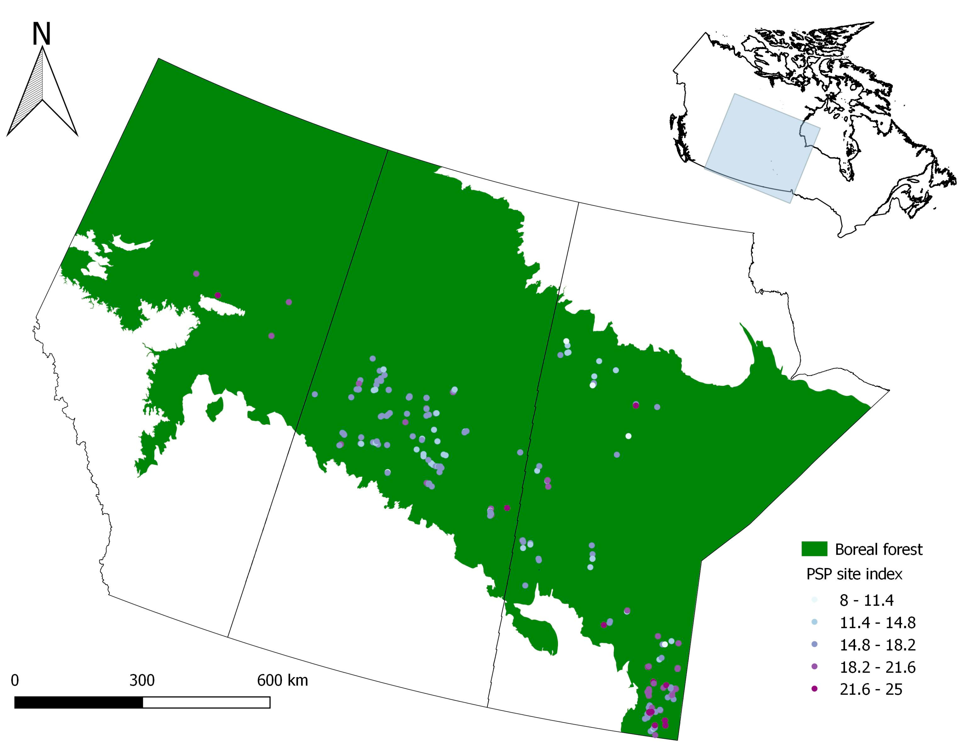
The data used for this study covered a large area across the western Canadian boreal forest (Figure 1), with 422 permanent sample plots located in the provinces of Alberta, Saskatchewan and Manitoba. The mean annual temperature at the plot locations ranged from −3.2 °C to 2.1 °C and mean annual precipitation from 410 to 537 mm/year (ClimateNA: http://tinyurl.com/ClimateNA accessed on 25 February 2015). Plot size varied from 27.8 m2 to 1500 m2, depending on source and year of measurement. PSP data was provided by Alberta Agriculture and Forestry (AAF), Saskatchewan Ministry of Environment and Manitoba Provincial Government. Information on plot design, measurement protocols, and plot history can be found in Alberta Environment and Sustainable Resource Development (AESRD) [31] and AESRD [32] for the plots in Alberta, in Teco Natural Resource Group Limited [33] for the plots in Saskatchewan, and in Vyvere [34] for the plots in Manitoba.
The data from the three sources were combined into a single dataset and plots were carefully reviewed to determine their suitability. In order to be selected for analysis, a plot had to be measured at least twice and include jack pine trees. Selected plots include a variety of stand types (structure and species mixtures) and various stand ages (juvenile, mid-rotation and mature) (Table 1).
Diameter at breast height (DBH) was used as the response variable for the diameter growth model. For the height growth model, only trees with measured heights were used, excluding any trees with estimated or interpolated heights. All trees were included in the calculation of stand level variables. There were 7785 tree mortality events recorded in our dataset.
Prior to model building, 10% of the available plots were randomly removed from the dataset to provide independent data for model validation. Prior to selection of this validation dataset, the data were stratified by age class (younger than 40 years, between 40 and 80 years and older than 80 years) and stand composition (jack pine basal area more than 80% of stand basal area and less than 80% of stand basal area). The independent validation plots were randomly selected from within each of the resulting six groups.
2.2. Diameter Growth Model
To develop the diameter growth model, we used the potential-modifier approach [35,36], in which the potential diameter growth was first estimated and then adjusted by a reduction factor to estimate growth. We used this approach as it is a common method used in growth modelling and in order to remain consistent with previous modelling of other species in the MGM. The potential DBH increment of the stand was calculated as the average DBH increment of the thickest 100 trees/ha. The reduction factor was expressed as a negative exponential function with a competition index represented as the sum of the DBHs of the trees with a larger DBH than the subject tree (DG). In order to account for different species competition effects on growth, the competition index was calculated separately for three species groups: deciduous (DDG), pine (PDG) and spruce/fir (SDG). Annual DBH increment was calculated as the diameter difference between two points in time divided by the period length.
The final form of the DBH growth equation was:
where DIijk is the DBH increment in the ith plot, of the jth tree for the kth measurement; Pot DIik is the potential DBH increment; DDG, PDG and SDG are competition indices; d, p, s are the fixed effects associated with di, pi, si as the plot level random effects assumed to be independent for different i and di,j, pi,j, si,j, as the tree level random effects are assumed to be independent for different i and j; and εijk is the residual error and are assumed to be independent for i, j and k, and independent of random effects. The random effects were assumed to be normally distributed with di, pi, si ~ N(0,Ψ1) and di,j, pi,j, si,j ~ N(0, Ψ2), where Ψ1 and Ψ2 are the variance–covariance matrices associated with the plot level random effect and tree level random effect, respectively.
2.3. Height Growth Model
The height increment model was also built using the potential modifier approach. The potential height increment of the stand was calculated as the average height increment of the thickest 100 trees/ha. The competition-based reduction factor used the sum of DBH greater than the subject tree for deciduous (DDG), pine (PDG) and spruce/fir (SDG). Annual height increment was calculated as the height difference between two points in time divided by the period length.
The final form for the height growth equation was:
where HIijk is the height increment in the ith plot, of the jth tree for the kth measurement; Pot HIik is the height increment; DDG, PDG and SDG are competition indices; d, p, s are the fixed effects associated with dj, pj, sj as the tree level random effects assumed to be independent for different j; and εjk is the residual error and is assumed to be independent for j and k, and independent of random effects. The random effects were assumed to be normally distributed as di, pi, si ~ N(0,Ψ1) where Ψ1 is the variance-covariance matrix associated with the tree level random effect.
2.4. Statistical Fitting of Growth Models
We used a non-linear mixed modelling approach to fit the growth equations as the data had a hierarchical (trees within plots) and correlated (repeated measure of the same tree) error structure. For diameter increment, both tree and plot were considered as random effects, meaning that the competition indices had a fixed component and a random component at both plot and tree level. For HI, only the tree level was used as a random effect as convergence could not be achieved with random effects at both tree and plot level. A diagonal variance–covariance structure was associated with the plot and tree random effects, which assumed independence among different grouping levels. In addition, an error correlation structure (compound symmetry) was used in the development of both models, considering the fact that measurements were taken repeatedly, at equal and unequal intervals. Structure search was based on the minimum Akaike Information Criterion (AIC) [37]. We used the nlme package version 3.1–108 [38] of the R statistical platform software [39] in order to fit, modify and asses the growth models.
2.5. Mortality Model
2.5.1. Variable Selection
In order to obtain a biologically meaningful model, we considered both tree- and stand-based variables as potential predictor variables for survival probability. Tree-based variables included in the final model were DBH [40] and DBH increment, both being variables commonly used in other mortality studies [41]. Furthermore, we used DBH2 to account for U-shape mortality pattern which is high in juvenile and old trees, but low in adult trees [40].
At the stand level, chosen explanatory variables were the sum of basal area of the thicker trees (BAGr) as a measure of competition; DBH2/stand basal area/ha (StBA) as a measure for tree social status in the stand; and jack pine relative composition (JPRC) as a measure of intraspecific interaction, defined as
where BAJP was defined as the total basal area per hectare for jack pine.
The last variable in the model, L, represents the length of the growth interval and was calculated as the difference between measurement years. These selected variables were assessed for significance using the likelihood ratio test [42], so that the model significance represents a combined understanding of biological processes and a statistical assessment.
2.5.2. Mortality Model Specification
We used logistic regression to model mortality. To account for the unequal time intervals present in our data, interval length was included in the model resulting in a generalized logistic model [43], an approach successfully applied in other studies, e.g., Yang [44], Yao [41]. However, L was included as a covariate, in order to allow for mixed effects modelling.
A generalized mixed model was used to estimate the coefficients, in order to account for the hierarchical data structure. The final form of the mortality function was:
where Prob survivalijk is the probability of survival of the jth tree at kth measurement in the ith plot; β0, β1, β2, β3, β4, β5, β6, β7 are the fixed effects coefficients; bi is the plot level random effect and εij is the residual error. The random effects were assumed to be normally distributed as bi ~ N(0,Ψ1), where Ψ1 is the variance–covariance matrix associated with the tree level random effect.
The coefficients for the intercept were considered mixed, with both a fixed and a random component. The significance of the random effects was assessed using the likelihood ratio test, by comparing the Bayesian Information Criterion (BIC) values and analyzing the ratio between the estimated random-effect standard deviation and the associated estimate of the fixed effect [37]. Package lme4 version 1.0–4 [45] in R was used in order to fit, modify and evaluate the mortality model.
The commonly used Hosmer–Lemeshow test for evaluating the goodness of fit of a logistic regression was not suitable for our data as it contained over 25,000 observations (Paul, Pennell, and Lemeshow, 2013). Instead, we used the Receiver Operating Curve (ROC), which plots the proportion of true positives (events predicted to be events) versus the proportion of false positives (nonevents predicted to be events). The area under the curve is given the by the c statistic, with any value greater than 0.5 showing a better than random discrimination. We applied the c statistic as a goodness of fit measure, using the R package hmeasure version 1.0 [46].
2.6. Validation Methods and Metrics
The fixed effects component of the developed growth and mortality models was implemented in the MGM. Using the independent validation dataset, we initialized the MGM with the first plot measurement and then projected the tree-list to the final re-measurement. The average projection interval was 18.2 years (min 5 years/maximum 36 years). The observed stand conditions were then evaluated against the MGM predictions. In order to determine potential height and DBH increment, the MGM uses SI as an input variable that measures site productivity [28]. In Alberta, SI was calculated according to Huang [47] and in Saskatchewan and Manitoba according to Cieszewski [48].
The models were validated at both tree and stand level. At the tree level, jack pine tree height (m) and DBH (cm) were used for validation, while at the stand level the model was validated for the following outputs: DBH increment (cm/year), height increment (m/year), stand volume (m3ha−1), basal area (m2ha−1), average DBH (cm), average height (m), top and height (m). Stand density (trees ha−1) was also examined as a basis for evaluating stand mortality. Top height was defined as the average height of the thickest 100 trees ha−1 of each species group. There were no removals over the projection periods and ingrowth was not included.
To assess the validity of the predictions, both graphical methods (plots of the observed (Y) versus predicted (Ŷ)) and statistical metrics were used. As statistical measures, we calculated average model bias (AMB), relative model bias in percentage (RMB) and efficiency (EF) [49]. Average model bias represents the average of the residual errors and was computed using the following formula:
where , are defined above, and n is the total number of observations.
The relative model bias (RMB) relates AMB to the observed mean estimator and is expressed as a percentage value, providing an indication of the magnitude of the AMB. It is calculated using the following formula:
where is the average of the observed values.
Efficiency is a dimensionless statistic that relates the model predictions to the observed data in a manner similar to that of the coefficient of determination (R2), and is described by:
where the variables are as defined in formulas [5,6]. The efficiency statistic has a theoretical upper bound of 1 indicating a perfect model fit, with a value of 0 indicating the model is no better than the mean.
3. Results
3.1. DBH and Height Increment
Parameter estimates and asymptotic standard errors were obtained for both DBH and height increment models (Table 2). In the final DBH increment model, all fixed effects for the competition indices of the three species groups (deciduous, pine, spruce-fir) were highly significant (p < 0.01) according to the conditional t-test.
All random effects were retained in the DBH increment model, as the ratio of the random effect standard deviation (Table 3) to the associated fixed effect estimate was relatively high, indicating their importance in the model [37]. This was further supported by the likelihood ratio test, which indicated that the random effects for deciduous, pine and spruce-fir competition indices were significant.
In the case of height increment, the fixed effects of the three competition indices were found to be significant, as indicated by the p-values of the conditional t-test (<0.05). Random effects were also significant and included in the model as their standard deviation was large in comparison to the associated fixed effects (Table 3).
Based on the AIC and BIC comparisons, the best correlation structure was compound symmetry (Table 2). Both growth models were tested for significant difference between the model with correlation structure and without correlation structure using a chi-square test. In both cases, the models were significantly different, with lower AIC and BIC for models with a specified correlation structure. The analysis of increment residuals in relation to maximum increment showed even spread for both models.
3.2. Mortality
Using the maximum likelihood method, we obtained parameter estimates and associated standard errors for all selected variables in the mortality model, as described in the methods section (Table 4). All variables listed in Table 4 were found to be significant at a 95% confidence interval using the likelihood ratio test.
The final mortality model was built having mixed coefficients for the intercept, with a random coefficient bi for within-plot variance. The large ratio of the random effect standard deviation (2.578) to the associated estimate of the fixed effects (−3.395) and the improved model fit (lower BIC) indicates the importance of the random effect. Adding random effects at the tree level did not produce a significantly different model and did not improve the BIC and therefore these were not included in the final model.
For this model formulation and selected predictor variables, the c-statistic was found to be 0.787, which can be translated into acceptable discrimination according to Hosmer and Lemeshow [42].
3.3. Validation of MGM
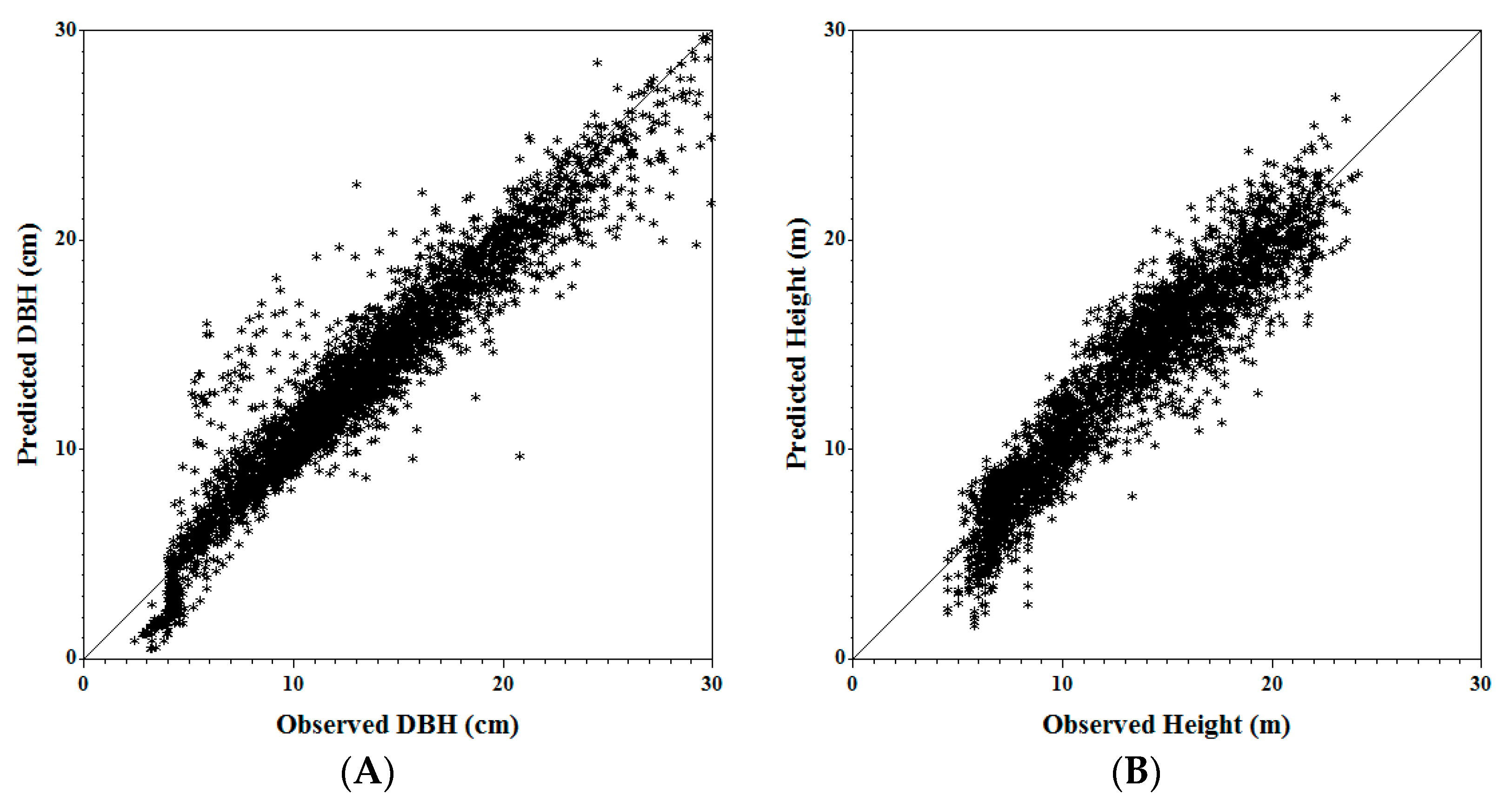
A total of 34 plots were randomly selected for the independent validation dataset. At tree level, the summary of validation metrics for the jack pine trees is shown in Table 5. A graphical representation of predicted vs. actual DBHs and heights is presented in Figure 2. Both tree DBH and tree height are under-predicted (AMB > 0), but the median RMB is relatively small (<10%). One plot has a RMB% of 42% due to a large presence of white birch. Birch is modelled in the MGM as an aspen, as the closest surrogate species; however, the two species are very different in their growth and competitive nature which results in poor model performance. DBH efficiency is relatively high (0.83), with values ranging from 0.02 to 0.98. Height efficiency is lower, with a higher spread of the data.
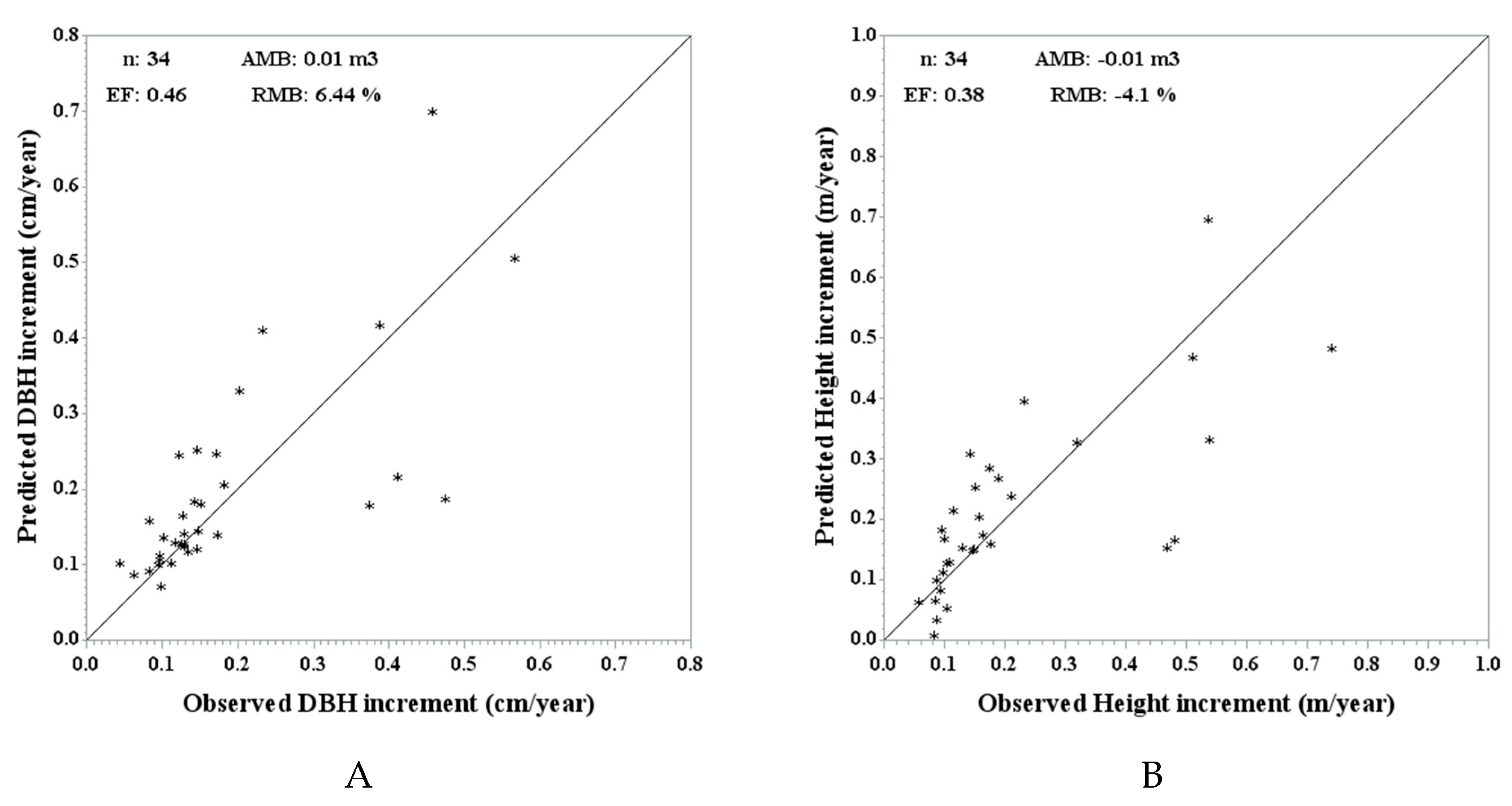
Figure 3 shows the predicted vs. actual plot for the DBH increment and height increment at stand level, together with the validation metrics. The RMB is under 10% for both increments and the efficiencies have lower values (0.46 for DBH and 0.38 for height).
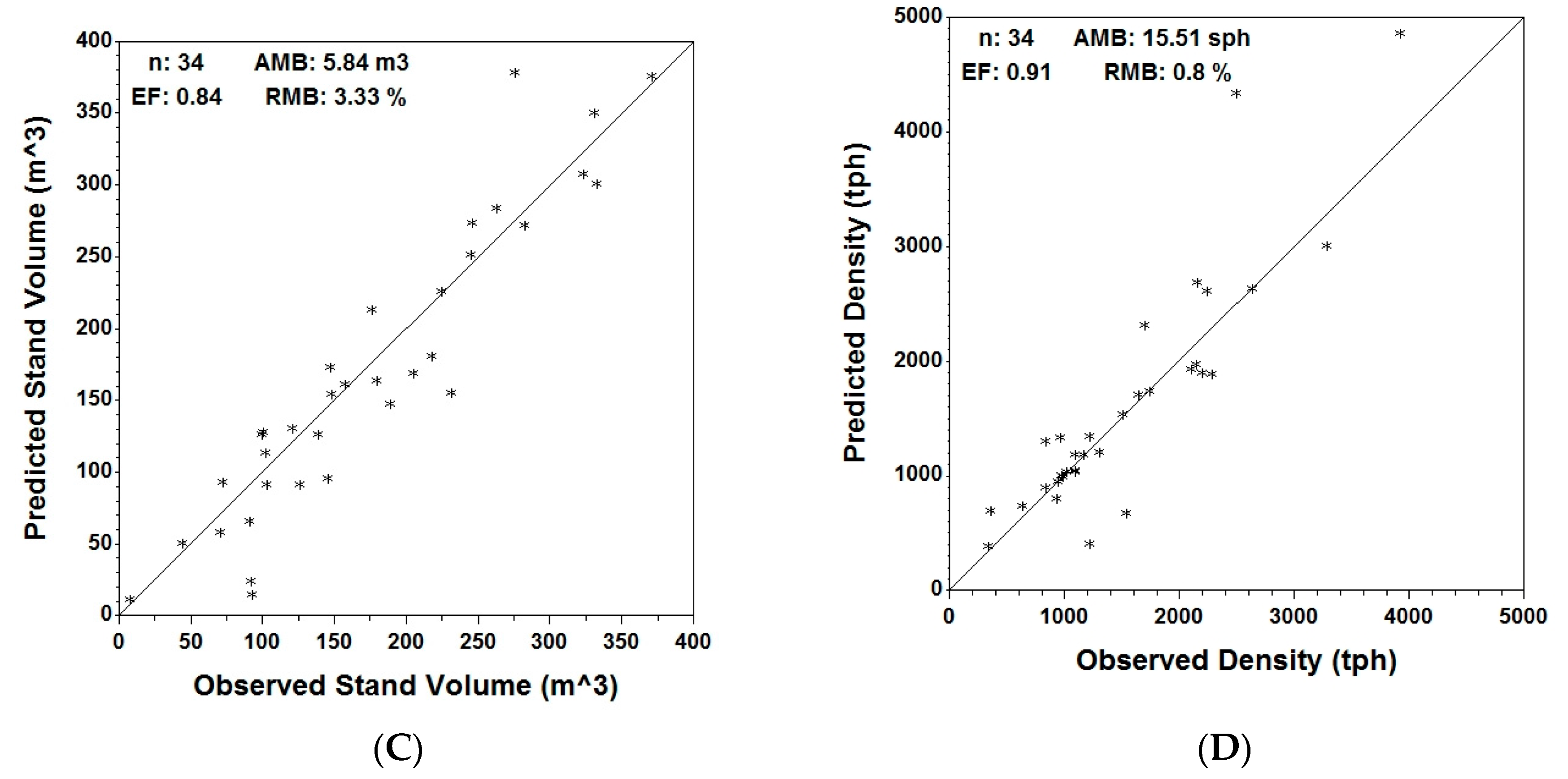
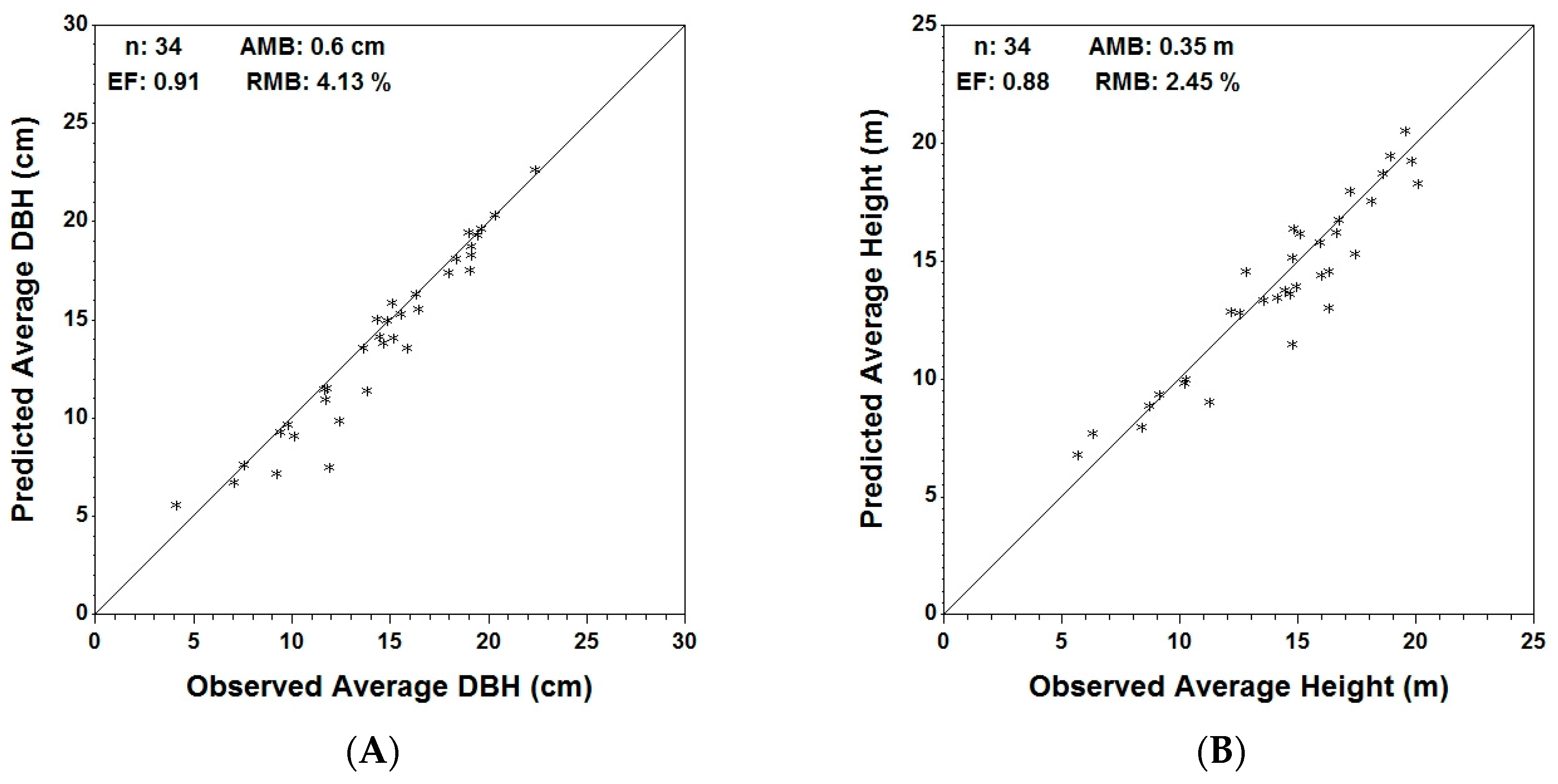
At stand level, Table 6 shows the actual, predicted and residual values of the analyzed variables for the entire plot, as well as for the coniferous and deciduous components. In Figure 4, predicted vs. actual stand volume/ha, average height, average DBH and density for the coniferous trees are displayed graphically. Graphs for the entire set of variables for both coniferous and deciduous trees are provided in the Supplementary material.
Validation statistics for coniferous trees (Table 7) indicate an under-prediction (AMB > 0) for all six variables, with the highest being average DBH (RMB = 4.13%) and the smallest being density (RMB = 0.8%). Efficiency for the coniferous component ranges between 0.66 for basal area/ha and a maximum of 0.91 for average DBH and density.
Unlike the prediction for conifers, there was an over-prediction of stand variables for the deciduous component, with a higher number of points lying above the 1:1 line. This was confirmed by the corresponding validation statistics, with most of the variables having a small negative AMB. Density was the only exception, which has a positive AMB of 50.66 tph for the deciduous component. In terms of efficiency, the highest value was obtained for average DBH (0.81), the lowest for top height (0.59).
4. Discussion
4.1. Ecological Significance
Jack pine is an early successional species; its strong pioneer character is mirrored in the ability to quickly regenerate on mineral soils after disturbances such as fire or management interventions. With fast early growth in the first 20 years of life [2], this species makes full use of the available light resources. As a result, jack pine is a highly shade-intolerant species. In our model, we have incorporated potential growth and competition measures that consider this silvicultural characteristic of jack pine.
The effect of inter- and intraspecific competition was incorporated in our growth models in the form of a distance-independent competition index, which has been used effectively in describing growth–competition relationships in boreal forests [36,50]. For Jack pine, Mugasha [51] showed that the distance-independent Lorimer’s index, calculated using only taller trees, was better than many other distance-dependent indices for characterizing variation in stem volume growth. In this study, we chose the sum of DBH of trees with a larger DBH than the subject tree as the competition index since it has been used successfully for other pioneer species [36]. We also tested the sum of basal area of trees larger than the subject tree, another commonly used competition index [36]. However, we rejected this index following exploratory analysis, as the AIC indicated a better fit for the DBH-based index. The sum of larger-DBH competition index is one sided and reflects only the dominant influence of light as a growth limiting factor. Nevertheless, for lodgepole pine Coates [7] stated that growth reduction is more likely to be influenced by shading rather than crowding, which should also apply to jack pine.
In the final DBH increment model, competition from the three species groups (deciduous, pine and spruce-fir) had a negative effect on pine growth, as indicated by the positive coefficients (Table 2). However, the three groups of competitors had different effect strengths, with deciduous (mainly aspen) competitors having the strongest effect and intraspecific competition having the lowest impact. Similar species-dependent competition effects were reported for lodgepole pine [7,52] and for eastern white pine [53]. This effect is likely related to species shade tolerance and stand development, with faster initial growth of aspen leading to the overtopping of the pine. As pine is a shade-intolerant species [2], the lack of light has a stronger effect on DBH growth. Spruce competition has a smaller effect on pine growth, due to its slower initial growth and with spruce remaining shorter than the pine until the stand reaches an advanced age. Results from the height growth model were similar to the DBH model, with the negative influence of competition being highest from the deciduous species group and weakest from the pine species group.
The DBH and height models have an inverse exponential form. Peak increment is achieved when a tree is competition free and decreases nonlinearly as the competition index increases. The response of predicted increment to species-specific competition is similar to the overall response, with increment decreasing in an inverse exponential way as competition increases for both growth models. Only in the case of deciduous competition, there is a short range of high competition where increment is increasing, but this is an artefact of the data, as the maximum increments are also higher. The analysis of increment residuals in relation to potential increment showed an even spread for both models.
In building the model, potential growth (measured by the increment of the thickest 100 tress/ha) was used as a measure of site productivity. In the MGM, potential growth is determined by SI, a variable that integrates many of the environmental factors that control growth. SI represents a widely accepted method for assessing site productivity [54,55] due to the ease of estimation from field observations and efficiency in growth and yield prediction. SI also has some limitations and can change with climate [55,56].
Tree mortality is a complicated process that is affected by a variety of environmental, pathological and physiological factors, as well as random events. However, tree mortality can frequently be explained by measures of tree size and growth rate, individual competition and stand density [57]. The variables selected to predict the probability of survival were DBH, DBH2, DBH increment, jack pine relative stand composition, DBH2 divided by stand basal area, basal area greater and the time interval length. The positive coefficients for DBH and negative coefficients for DBH2 (Table 4) indicate a U-shaped mortality pattern: when trees are small (and young), they usually have relatively high mortality [58]. At this stage, DBH dominates the trend due to its higher coefficient compared with DBH2. As trees increase in DBH, survival probability increases and becomes stable over the middle of the size range. At older stages and larger tree sizes, survival probability decreases again with DBH2 becoming dominant over DBH. This widely reported trend of increasing mortality in larger (older) trees (e.g., Cortini [59] for boreal jack pine) is caused by several factors. Old trees lose vigor due to physiological aging, increasing hydraulic resistance, decreasing leaf area, and leading to higher maintenance respiration costs [60]. This leads to a decline in vitality and a reduced ability to survive insect attacks, diseases or climate extremes [41].
DBH increment was included in the mortality model as it is an indicator of tree vigor. The positive coefficients (Table 4) show that trees with a higher DBH increment also have a lower chance of mortality. This observation is consistent with other studies (e.g., [61]) that show diameter increment is strongly related to survival probability.
According to our model, the mortality of jack pine is lower in pure pine stands compared to mixed species stands, as indicated by the positive coefficient of relative pine stand composition (Table 4). This is likely related to the shade intolerance of pines in general, with Yao [41] reporting similar results for lodgepole pine. In mixed species stands, pine is overtopped by fast growing aspen resulting in a higher mortality.
Basal area greater (BA greater) and DBH2 divided by the stand basal area/ha (DBH2/StBA) are variables that measure the social status of a tree in the stand. The negative coefficient for BA greater indicates an increase in mortality as the number of trees larger than the subject tree increases. On the other hand, the probability of survival increases if the tree is situated in an upper size class (as indicated by DBH2/StBA). In addition, DBH2/StBA provides a measure of the contribution of the tree to stand basal area. The last variable in the model, length of time interval (L), was used to account for unequal measurement intervals. The analysis showed that the probability of survival decreases with every year for which the tree is modelled; as the time interval increases, so does the risk of biotic or abiotic damage and the risk of mortality.
4.2. Application in Forest Management
The developed growth and mortality models were successfully implemented in the MGM. At tree level, the model tends to slightly under-predict, with AMB being positive, but the bias is limited. Small dimension trees are under-predicted probably due to large variations in growth for saplings [62]. The height growth model has lower efficiency, probably due to lower precision of height measurements, as well as greater variation in height growth. There was no bias in relation to stand density or stand age. At stand level, DBH and height increment also showed a small bias, but lower efficiencies due to errors at higher increments. The model performed well for all stand variables and validation indicates that the MGM predicts stand volume/ha, stand density, average DBH and average height with a low bias. This supports the use of the MGM by forest managers in yield forecasting and management planning for pure and mixed jack pine stands in Western Canada.
5. Conclusions
Accurate forecasts of yield and forest stand composition over time are important for management planning, allowable cut determination and maintaining a balance of species mixture over the landscape. This study was aimed at developing deterministic growth and mortality models for jack pine using data from a large number of remeasured PSPs.
The development of the growth models was achieved using nonlinear mixed modelling to relate potential growth and competition. The mortality model was developed using a mixed logistic regression and having stand and tree level as explanatory variables. Both growth and mortality models make sense ecologically and are based on the silvicultural characteristics of jack pine, which can be used to interpret the model’s estimated coefficients.
The resulting models were implemented into the MGM as part of the overall system of equations, and validated against an independent dataset. The good performance of the model predictions showed that now the MGM is able to predict with low bias variables such as stand volume, density, average DBH, and average height for stands that contain jack pine. Further refinements that can improve the MGM and expand its use in forest management in the western boreal region will likely be achieved by including climate effects in the growth and mortality functions and by refining the site index curves, with the inclusion of climate.
Supplementary Materials
The following are available online at www.mdpi.com/1999-4907/8/11/410/s1, Figure S1: Observed vs predicted independent validation data (n = 34) using MGM stand predictions with respective validation metrics: average mean bias (AMB), relative mean bias (RMB) and efficiency (EF).
Acknowledgments
Financial support for this project was provided by Saskatchewan Environment, Alberta Agriculture and Forestry, and Alberta Pacific Forest Industries. The project was also supported by the WEStern BOreal Growth and Yield Association (WESBOGY). Data were provided by Saskatchewan Environment, Alberta Environment and Sustainable Resource Development, and Manitoba Conservation and Water Stewardship. We would like to acknowledge and thank Ken Stadt for his contribution in the model development and his assistance in preparing Alberta data, to Stephen J. Titus for his help in implementing the Jack pine code into the MGM, to Phil Loseth and Lane Gelhorn for their help with the Saskatchewan data, and to Shawn Meng for his help with the Manitoba data.
Author Contributions
P.G.C. and M.B. conceived and designed the study, V.C.S. analyzed the data with contribution from M.B. and P.G.C., V.C.S. wrote the paper with contributions from P.G.C. and M.B.
Conflicts of Interest
The authors declare no conflict of interest. The founding sponsors had no role in the design of the study, analyses, or interpretation of data; in the writing of the manuscript, and in the decision to publish the results. The founding sponsors were involved in the collection of the field data.
References
- Canadian Forest Service Canada’s National Forest Inventory. Available online: https://nfi.nfis.org/home.php?lang=en (accessed on 5 February 2015).
- Burns, R.M.; Honkala, B.H. Silvics of North America; United States Department of Agriculture: Washington, DC, USA, 1990. [Google Scholar]
- Cayford, J.H.; Chrosciewicz, Z.; Sims, H.P. A Review of Silvicultural Research in Jack Pine; Northern Forest Research Centre: Edmonton, AB, Canada, 1967.
- Hamilton, W.N.; Krause, H.H. Relationship between jack pine growth and site variables in New Brunswick plantations. Can. J. For. Res. 1985, 15, 922–926. [Google Scholar] [CrossRef]
- Bell, F.W.; Ter-Mikaelian, M.T.; Wagner, R.G. Relative competitiveness of nine early-successional boreal forest species associated with planted jack pine and black spruce seedlings. Can. J. For. Res. 2000, 30, 790–800. [Google Scholar] [CrossRef]
- Day, M.E.; Schedlbauer, J.L.; Livingston, W.H.; Greenwood, M.S.; White, A.S.; Brissette, J.C. Influence of seedbed, light environment, and elevated night temperature on growth and carbon allocation in pitch pine (Pinus rigida) and jack pine (Pinus banksiana) seedlings. For. Ecol. Manag. 2005, 205, 59–71. [Google Scholar] [CrossRef]
- Coates, K.D.; Canham, C.D.; LePage, P.T. Above-versus below-ground competitive effects and responses of a guild of temperate tree species. J. Ecol. 2009, 97, 118–130. [Google Scholar] [CrossRef]
- Béland, M.; Bergeron, Y.; Zarnovican, R. Harvest treatment, scarification and competing vegetation affect jack pine establishment on three soil types of the boreal mixed wood of northwestern Quebec. For. Ecol. Manag. 2003, 174, 477–493. [Google Scholar] [CrossRef]
- Genries, A.; Drobyshev, I.; Bergeron, Y. Growth-climate response of Jack pine on clay soils in northeastern Canada. Dendrochronologia 2012, 30, 127–136. [Google Scholar] [CrossRef]
- Royer-Tardif, S.; Bradley, R.L. Evidence that soil fertility controls the mixing of jack pine with trembling aspen. For. Ecol. Manag. 2011, 262, 1054–1060. [Google Scholar] [CrossRef]
- Pinno, B.D.; Errington, R.C.; Thompson, D.K. Young jack pine and high severity fire combine to create potentially expansive areas of understocked forest. For. Ecol. Manag. 2013, 310, 517–522. [Google Scholar] [CrossRef]
- Smirnova, E.; Bergeron, Y.; Brais, S. Influence of fire intensity on structure and composition of jack pine stands in the boreal forest of Quebec: Live trees, understory vegetation and dead wood dynamics. For. Ecol. Manag. 2008, 255, 2916–2927. [Google Scholar] [CrossRef]
- Bella, I.E.; DeFranceschi, J.P. Commercial Thinning Improves Growth of Jack Pine; Northern Forest Research Centre, Canadian Forestry Service, Department of the Environment: Edmonton, AB, Canada, 1974.
- Moulinier, J.; Brais, S.; Harvey, B.D.; Koubaa, A. Response of boreal jack pine (Pinus banksiana Lamb.) stands to a gradient of commercial thinning intensities, with and without N fertilization. Forests 2015, 6, 2678–2702. [Google Scholar] [CrossRef]
- Bella, I.E.; DeFranceschi, J.P. Analysis of Jack Pine Thinning Experiments, Manitoba and Saskatchewan; Northern Forest Research Centre: Edmonton, AB, Canada, 1974.
- Tong, Q.J.; Zhang, S.Y.; Thompson, M. Evaluation of growth response, stand value and financial return for pre-commercially thinned jack pine stands in Northwestern Ontario. For. Ecol. Manag. 2005, 209, 225–235. [Google Scholar] [CrossRef]
- Mitchell, K.J. Dynamics and simulated yield of Douglas-fir. For. Sci. Monogr. 1975, 17, 1–39. [Google Scholar]
- Di Lucca, C.M. TASS/SYLVER/TIPSY: Systems for predicting the impact of silvicultural practices on yield, lumber value, economic return and other benefits. In Proceedings of the Stand Density Management Conference: Using the Planning Tools, Edmonton, AB, Canada, 23–24 November 1998; pp. 7–16. [Google Scholar]
- Marshall, P.; Parysow, P.; Akindele, S. Evaluating Growth Models: A Case Study Using PrognosisBC. In Proceedings of the HIRD Forest Vegetation Simulator Conference, Fort Collins, CO, USA, 13–15 February 2007. [Google Scholar]
- Temesgen, H.; LeMay, V. Examination of Large Tree Height and Diameter Increment Models Modified for PrognosisBC; Report Prepared for the Britisch Columbia Ministry of Forests, University of British Columbia: Vancouver, BC, Canada, 1999; Volume 143. [Google Scholar]
- Peng, C.; Liu, J.; Dang, Q.; Apps, M.J.; Jiang, H. TRIPLEX: A generic hybrid model for predicting forest growth and carbon and nitrogen dynamics. Ecol. Model. 2002, 153, 109–130. [Google Scholar] [CrossRef]
- Dufour-Kowalski, S.; Courbaud, B.; Dreyfus, P.; Meredieu, C.; de Coligny, F. Capsis: An open software framework and community for forest growth modelling. Ann. For. Sci. 2012, 69, 221–233. [Google Scholar] [CrossRef]
- Ashraf, M.I.; Meng, F.-R.; Bourque, C.P.-A.; MacLean, D.A. A Novel Modelling Approach for Predicting Forest Growth and Yield under Climate Change. PLoS ONE 2015, 10, e0132066. [Google Scholar] [CrossRef] [PubMed]
- Lacerte, V.; Larocque, G.R.; Woods, M.; Parton, W.J.; Penner, M. Calibration of the forest vegetation simulator (FVS) model for the main forest species of Ontario, Canada. Ecol. Model. 2006, 199, 336–349. [Google Scholar] [CrossRef]
- Pokharel, B.; Froese, R.E. Representing site productivity in the basal area increment model for FVS-Ontario. For. Ecol. Manag. 2009, 258, 657–666. [Google Scholar] [CrossRef]
- Government of Alberta Growth & Yield Projection System. Available online: http://www.agric.gov.ab.ca/app21/forestrypage?cat1=Forest Management&cat2=Growth %26 Yield&cat3=Growth %26 Yield Projection System (accessed on 15 August 2017).
- Subedi, N.; Sharma, M. Individual-tree diameter growth models for black spruce and jack pine plantations in northern Ontario. For. Ecol. Manag. 2011, 261, 2140–2148. [Google Scholar] [CrossRef]
- Bokalo, M.; Stadt, K.; Comeau, P.; Titus, S. The Validation of the Mixedwood Growth Model (MGM) for Use in Forest Management Decision Making. Forests 2013, 4, 1–27. [Google Scholar] [CrossRef]
- Comeau, P.G.; Kabzems, R.; McClarnon, J.; Heineman, J.L. Implications of selected approaches for regenerating and managing western boreal mixedwoods. For. Chron. 2005, 81, 559–574. [Google Scholar] [CrossRef]
- Pitt, D.G.; Mihajlovich, M.; Proudfoot, L.M. Juvenile stand responses and potential outcomes of conifer release efforts on Alberta’s spruce–aspen mixedwood sites. For. Chron. 2004, 80, 583–597. [Google Scholar] [CrossRef]
- Alberta Environment and Sustainable Resource Development. Permanent Sample Plot (PSP) Field Procedures Manual; Alberta Environment and Sustainable Resource Development: Edmonton, AB, Canada, 2005. [Google Scholar]
- Alberta Environment and Sustainable Resource Development. Stand Dynamic System Manual; Alberta Environment and Sustainable Resource Development: Edmonton, AB, Canada, 2005. [Google Scholar]
- TECO Natural Resource Group Limited. Saskathewan Permanent Sample Plots Data Consolidation and Database Development; TECO Natural Resource Group Limited: Edmonton, AB, Canada, 2011. [Google Scholar]
- Vyvere, D.V. Permanent Sample Plot Manual; Governament report for Manitoba Provincial Government Winnipeg; 2011. Available online: https://www.agric.gov.ab.ca/app21/forestrypage?cat1=Forest%20Management&cat2=Permanent%20Sample%20Plots (accessed on 15 August 2017).
- Ek, A.; Monserud, R.A. FOREST A Computer Model for Simulating the Growth and Reproduction of Mixed Species Forest Stands; School of Natural Resources, University of Wisconsin-Madison: Madison, WI, USA, 1974. [Google Scholar]
- Huang, J.-G.; Stadt, K.J.; Dawson, A.; Comeau, P.G. Modelling growth-competition relationships in trembling aspen and white spruce mixed boreal forests of Western Canada. PLoS ONE 2013, 8, e77607. [Google Scholar] [CrossRef] [PubMed]
- Pinheiro, J.; Bates, D. Mixed Effects Models in S and S-PLUS; Spinger: New York, NY, USA, 2000. [Google Scholar]
- Pinheiro, J.; Bates, D.; DebRoy, S.; Sarkar, D.; R Development Core Team. nlme: Linear and Nonlinear Mixed Effects Models; R Core Team: Vienna, Austria, 2013. [Google Scholar]
- R Core Team. R: A Language and Environment for Statistical Computing; R Core Team: Vienna, Austria, 2013. [Google Scholar]
- Monserud, R.; Sterba, H. Modeling individual tree mortality for Austrian forest species. For. Ecol. Manag. 1999, 113, 109–123. [Google Scholar] [CrossRef]
- Yao, X.; Titus, S.J.; MacDonald, S.E. A generalized logistic model of individual tree mortality for aspen, white spruce, and lodgepole pine in Alberta mi×edwood forests. Can. J. For. Res. 2001, 31, 283–291. [Google Scholar] [CrossRef]
- Hosmer, D.; Lemeshow, S. Applied Logistic Regression, 2nd ed.; John Wiley& Sons: Toronto, ON, Canada, 2000; ISBN 0-471-35632-8. [Google Scholar]
- Monserud, R. Simulation of forest tree mortality. For. Sci. 1976, 22, 438–444. [Google Scholar]
- Yang, Y.; Titus, S.J.; Huang, S. Modeling individual tree mortality for white spruce in Alberta. Ecol. Model. 2003, 163, 209–222. [Google Scholar] [CrossRef]
- Bates, D.; Maechler, M.; Bolker, B.; Walker, S.; Christensen, R.H.B.; Singmann, H.; Dai, B.; Grothendieck, G.; Green, P. lme4: Linear Mixed-Effects Models Using Eigen and S4, R package version 1.1-14; 2017. Available online: https://cran.r-project.org/web/packages/lme4/index.html (accessed on 15 August 2017).
- Anagnostopoulos, C.; Hand, D.J. hmeasure: The H-Measure and Other Scalar Classification Performance Metrics, R package version 1.0; 2012. Available online: http://CRAN.R-project.org/package=hmeasure (accessed on 15 August 2017).
- Huang, S. A Versatile Height and Site Index Model for Jack Pine in Alberta; Alberta Environmental Protection Land and Forest Service: Edmonton, AB, Canada, 1997. [Google Scholar]
- Cieszewski, C.; Bella, I.E.; Yeung, D.P. Preliminary Site-Index Height Growth Curves for Eleven Timber Species in Saskatchewan; Canada–Saskatchewan Partnership Agreement in Forestry; Natural Resources Canada, Canada Forest Service: Prince Alberta, SK, Canada, 1993.
- Vanclay, J.K.; Skovsgaard, J.P. Evaluating forest growth models. Ecol. Model. 1997, 98, 1–12. [Google Scholar] [CrossRef] [Green Version]
- Filipescu, C.N.; Comeau, P.G. Aspen competition affects light and white spruce growth across several boreal sites in western Canada. Can. J. For. Res. 2007, 37, 1701–1713. [Google Scholar] [CrossRef]
- Mugasha, A.G. Evaluation of simple competition indices for the prediction of volume increment of young jack pine and trembling aspen trees. For. Ecol. Manag. 1989, 26, 227–235. [Google Scholar] [CrossRef]
- Stadt, K.J.; Huston, C.; Coates, D.K.; Feng, Z.; Dale, M.R.T.; Lieffers, V.J.; Kenneth, J.S.; Carolyn, H.; David, K.C.; Zhili, F.; et al. Evaluation of competition and light estimation indices for predicting diameter growth in mature boreal mixed forests. Ann. For. Sci. 2007, 64, 477–490. [Google Scholar] [CrossRef]
- Canham, C.D.; Papaik, M.J.; Uriarte, M.; McWilliams, W.H.; Jenkins, J.C.; Twery, M.J. Neighborhood analyses of canopy tree competition along environmental gradients in New England forests. Ecol. Appl. 2006, 16, 540–554. [Google Scholar] [CrossRef]
- Carmean, W.H.; Lenthall, D.J. Height-growth and site-index curves for jack pine in north central Ontario. Can. J. For. Res. 1989, 19, 215–224. [Google Scholar] [CrossRef]
- Sharma, M.; Subedi, N.; Ter-Mikaelian, M.; Parton, J. Modeling climatic effects on stand Height/Site index of plantation-grown jack pine and black spruce trees. For. Sci. 2015, 61, 25–34. [Google Scholar] [CrossRef]
- Weiskittel, A.R.; Crookston, N.L.; Radtke, P.J. Linking climate, gross primary productivity, and site index across forests of the western United States. Can. J. For. Res. 2011, 41, 1710–1721. [Google Scholar] [CrossRef]
- Hamilton, D.A. A Logistic Model of Mortality in Thinned and Unthinned Mixed Conifer Stands of Northern Idaho. For. Sci. 1986, 32, 989–1000. [Google Scholar]
- Kenkel, N.C.; Hoskins, J.A.; Hoskins, W.D. Local competition in a naturally established jack pine stand. Can. J. Bot. 1989, 67, 2630–2635. [Google Scholar] [CrossRef]
- Cortini, F.; Comeau, P.G.; Strimbu, V.C.; Hogg, E.H.; Bokalo, M.; Huang, S. Survival functions for boreal tree species in northwestern North America. For. Ecol. Manag. 2017, 402, 177–185. [Google Scholar] [CrossRef]
- Ryan, M.G.; Yoder, B.J. Hydraulic limits to tree height and tree growth. Bioscience 1997, 47, 235–242. [Google Scholar] [CrossRef]
- Kobe, R.K.; Coates, K.D. Models of sapling mortality as a function of growth to characterize interspecific variation in shade tolerance of eight tree species of northwestern British Columbia. Can. J. For. Res. 1997, 27, 227–236. [Google Scholar] [CrossRef]
- Zhang, L.; Peng, C.; Dang, Q. Individual-tree basal area growth models for jack pine and black spruce in northern Ontario. For. Chron. 2004, 80, 366–374. [Google Scholar] [CrossRef]
Figure 1.
Permanent sample plot location by jack pine site index in the Canadian provinces of Alberta, Saskatchewan and Manitoba.
Figure 1.
Permanent sample plot location by jack pine site index in the Canadian provinces of Alberta, Saskatchewan and Manitoba.

Figure 2.
Observed vs. predicted tree DBH (A) and tree height (B) for jack pine using validation data in the Mixedwood Growth Model (MGM).
Figure 2.
Observed vs. predicted tree DBH (A) and tree height (B) for jack pine using validation data in the Mixedwood Growth Model (MGM).

Figure 3.
Observed vs. predicted DBH increment (A) and height increment (B) using the independent validation data and MGM stand predictions (n = 34) with respective validation metrics: average mean bias (AMB), relative mean bias (RMB) and efficiency (EF).
Figure 3.
Observed vs. predicted DBH increment (A) and height increment (B) using the independent validation data and MGM stand predictions (n = 34) with respective validation metrics: average mean bias (AMB), relative mean bias (RMB) and efficiency (EF).

Figure 4.
Observed vs. predicted independent validation data (n = 34) using MGM stand predictions for average DBH (A); average height (B); stand volume (C) and stand density (D) with respective validation metrics: average mean bias (AMB), relative mean bias (RMB) and efficiency (EF).
Figure 4.
Observed vs. predicted independent validation data (n = 34) using MGM stand predictions for average DBH (A); average height (B); stand volume (C) and stand density (D) with respective validation metrics: average mean bias (AMB), relative mean bias (RMB) and efficiency (EF).


Table 1.
Summary of data used in the study with tree and stand variables.
| Variable | Units | Mean | Std. Dev. | Minimum | Maximum |
|---|---|---|---|---|---|
| Jack pine diameter at breast height (DBH) | cm | 10.67 | 6.14 | 0.20 | 58.50 |
| Jack pine height | m | 10.65 | 5.17 | 1.30 | 31.60 |
| Jack Pine DBH increment | cm/year | 0.14 | 0.14 | −0.2 | 1.16 |
| Jack Pine height increment | m/year | 0.19 | 0.19 | −0.4 | 1.2 |
| Measurement interval | years | 6.33 | 3.37 | 2.00 | 36.00 |
| Jack Pine Mortality | % trees dead/plot | 14% | 17.8% | 0.8% | 100% |
| Number of plot remesurements | 1.78 | 0.93 | 1.00 | 5.00 | |
| Site Index | m | 16.53 | 2.78 | 7.73 | 25.69 |
| Stand age | years | 54.17 | 24.84 | 6.00 | 154.00 |
| Coniferous density | tph | 2587.58 | 5098.28 | 12.36 | 75,184.96 |
| Deciduous density | tph | 230.86 | 679.44 | 0.00 | 12,230.00 |
| Coniferous Avg DBH | cm | 13.30 | 5.35 | 0.63 | 35.50 |
| Deciduous Avg DBH | cm | 5.99 | 7.42 | 0.00 | 37.80 |
| Coniferous Avg Height | m | 12.52 | 4.31 | 1.50 | 23.49 |
| Deciduous Avg Height | m | 6.15 | 7.01 | 0.00 | 27.30 |
| Coniferous basal area | m2/ha | 21.22 | 9.66 | 0.10 | 47.44 |
| Deciduous basal area | m2/ha | 2.06 | 5.26 | 0.00 | 38.35 |
| Stand Quadratic Mean Diameter (QMD) | cm | 13.59 | 5.17 | 0.71 | 32.11 |
| Stand volume | m3/ha | 148.98 | 88.13 | 0.54 | 450.14 |
| Stand Basal area | m2/ha | 23.28 | 9.50 | 0.55 | 48.63 |
| Stand Density | tph | 2783.42 | 5155.72 | 125.00 | 76,584.68 |
Table 2.
Estimated fixed effects coefficients and standard error for DBH and height increment models (with and without a specified correlation structure). The variables are represented by the sum of the DBHs of the deciduous trees (DDG), pine trees (PDG) and spruce-fir trees (SDG) with a larger DBH than the subject tree.
| No Correlation Structure | Correlation Structure | |||||
|---|---|---|---|---|---|---|
| Variable | Parameter (Degrees of Freedom) | Estimate | SE | Estimate | SE | |
| Diameter at breast height (DBH) increment | Rho | Not used | 0.1554 | |||
| DDG | d (42817) | 6.2791 | 10.800 | 6.1838 | 10.900 | |
| PDG | p (42817) | 4.9404 | 0.1640 | 5.0129 | 0.16500 | |
| SDG | s (42817) | 36.324 | 4.2700 | 35.929 | 4.2400 | |
| Height increment | Rho | Not used | −0.06087 | |||
| DDG | d (40404) | 7.4728 | 0.40100 | 7.5410 | 0.39500 | |
| PDG | p (40404) | 3.0850 | 0.018900 | 3.0890 | 0.018600 | |
| SDG | s (40404) | 5.1236 | 0.43300 | 4.8842 | 0.42000 | |
Table 3.
Estimated random effects standard deviation for the DBH (Diameter at breast height) increment model (plot and tree level) and for the height increment model (tree level).
Table 3.
Estimated random effects standard deviation for the DBH (Diameter at breast height) increment model (plot and tree level) and for the height increment model (tree level).
| Variable | Random Effect | Standard Deviation | |
|---|---|---|---|
| DBH increment | Plot level | ||
| DDG (deciduous trees) | σ1 | 6.59 | |
| PDG (pine trees) | σ1 | 1.42 | |
| SDG (spruce-fir trees) | σ1 | 5.68 | |
| Tree level | |||
| DDG | σ2 | 122 | |
| PDG | σ2 | 2.63 | |
| SDG | σ2 | 40.8 | |
| Residual | 6850 | ||
| Height increment | Tree level | ||
| DDG | σ | 5.49 | |
| PDG | σ | 1.25 | |
| SDG | σ | 3.23 | |
| Residual | 1480 | ||
Table 4.
Parameter estimates and standard errors (SE) for the mortality model.
| Variable | Estimate | SE |
|---|---|---|
| Intercept | −3.39488 | 0.649369 |
| DBH (Diameter at breast height) | 0.525338 | 0.016738 |
| DBH2 | −0.01791 | 0.000783 |
| DBH increment | 7.899263 | 0.280795 |
| StComp | 3.700769 | 0.632396 |
| DBH2/StBA | 0.044852 | 0.015472 |
| BA greater | −0.00547 | 0.000235 |
| L | −0.08825 | 0.009757 |
Table 5.
Summary of the validation statistics (AMB = average mean bias in original units, RMB = relative mean bias in %, EF = efficiency) for DBH and height at the individual tree level based on the validation plot values.
Table 5.
Summary of the validation statistics (AMB = average mean bias in original units, RMB = relative mean bias in %, EF = efficiency) for DBH and height at the individual tree level based on the validation plot values.
| Mean | Median | Std. Dev. | Min | Max | ||
|---|---|---|---|---|---|---|
| DBH (Diameter at breast height) | AMB | 0.07 | 0.06 | 1.22 | −2.46 | 5.07 |
| RMB % | 0.95% | 0.34% | 9.38% | −12.58% | 42.55% | |
| EF | 0.7 | 0.81 | 0.38 | −1.15 | 0.98 | |
| Height | AMB | 0.31 | 0.14 | 1.06 | −1.94 | 2.73 |
| RMB % | 1.65% | 1.33% | 7.86% | −21.98% | 18.49% | |
| EF | 0.05 | 0.25 | 0.7 | −2.23 | 0.82 |
Table 6.
Summary of actual, predicted and residual descriptive statistics for volume (m3/ha), basal area (m2/ha), average DBH (cm), average height (m), top height (m) at component level, density (tph), DBH increment (cm/year) and height increment (m/year) for the whole stand, and for coniferous and deciduous components.
| Observed | Predicted | Residuals | |||||||||||
|---|---|---|---|---|---|---|---|---|---|---|---|---|---|
| Mean | Min | Max | Std. Dev. | Mean | Min | Max | Std. Dev. | Mean | Min | Max | Std. Dev. | ||
| Stand | Volume | 178.83 | 7.69 | 371.15 | 90.41 | 174.12 | 11.15 | 378.04 | 100.12 | 4.71 | −102.22 | 76.10 | 35.32 |
| BA | 25.94 | 1.67 | 42.14 | 9.03 | 25.45 | 2.66 | 42.98 | 10.54 | 0.48 | −12.59 | 14.84 | 5.15 | |
| Avg DBH | 14.22 | 4.14 | 22.36 | 4.55 | 13.73 | 5.58 | 22.63 | 4.65 | 0.50 | −1.44 | 3.57 | 1.11 | |
| Avg Ht | 14.16 | 5.80 | 20.10 | 3.92 | 13.85 | 6.83 | 20.18 | 3.75 | 0.30 | −2.40 | 3.31 | 1.34 | |
| Density | 2161.69 | 333.33 | 17,068.39 | 2827.84 | 2122.35 | 389.43 | 13,416.97 | 2269.25 | 39.35 | −1833.48 | 3651.42 | 911.00 | |
| DBH increment | 0.20 | 0.07 | 0.70 | 0.13 | 0.18 | 0.04 | 0.57 | 0.13 | 0.01 | −0.29 | 0.24 | 0.10 | |
| Height increment | 0.20 | 0 | 0.70 | 0.15 | 0.20 | 0.05 | 0.74 | 0.17 | −0.01 | −0.32 | 0.17 | 0.12 | |
| Coniferous | Volume | 175.26 | 7.69 | 371.15 | 91.40 | 169.42 | 11.15 | 378.04 | 102.00 | 5.84 | −102.22 | 77.96 | 35.81 |
| BA | 25.21 | 1.67 | 42.02 | 9.20 | 24.49 | 2.66 | 42.98 | 11.03 | 0.72 | −12.59 | 15.90 | 5.29 | |
| Avg DBH | 14.46 | 4.11 | 22.36 | 4.30 | 13.87 | 5.58 | 22.63 | 4.49 | 0.60 | −1.46 | 4.39 | 1.13 | |
| Avg Ht | 14.30 | 5.69 | 20.10 | 3.80 | 13.95 | 6.81 | 20.49 | 3.67 | 0.35 | −1.79 | 3.31 | 1.27 | |
| Density | 1943.19 | 333.33 | 15,449.49 | 2516.60 | 1927.69 | 389.43 | 12,167.26 | 2070.99 | 15.51 | −1833.48 | 3282.24 | 741.63 | |
| TopHt | 16.58 | 8.38 | 23.09 | 3.81 | 16.12 | 9.50 | 22.86 | 3.69 | 0.47 | −1.64 | 3.17 | 1.08 | |
| DBH increment | 0.19 | 0.07 | 0.54 | 0.11 | 0.18 | 0.02 | 0.57 | 0.14 | 0.01 | −0.42 | 0.22 | 0.11 | |
| Height increment | 0.19 | 0 | 0.54 | 0.14 | 0.21 | 0.04 | 0.76 | 0.19 | −0.02 | −0.58 | 0.17 | 0.14 | |
| Deciduous | Volume | 8.09 | 0.41 | 31.99 | 8.62 | 10.00 | 1.44 | 34.81 | 9.84 | −2.41 | −8.83 | 2.89 | 3.13 |
| BA | 1.64 | 0.09 | 7.46 | 1.91 | 2.05 | 0.26 | 7.68 | 2.25 | −0.51 | −3.29 | 0.41 | 0.87 | |
| Avg DBH | 11.18 | 3.70 | 20.42 | 5.55 | 13.05 | 5.35 | 20.51 | 5.12 | −1.39 | −5.35 | 2.60 | 1.93 | |
| Avg Ht | 11.67 | 5.64 | 19.33 | 4.38 | 13.21 | 6.14 | 18.65 | 4.02 | −1.34 | −4.60 | 1.25 | 1.91 | |
| Density | 218.50 | 0.00 | 3720.64 | 696.25 | 194.66 | 0.00 | 2284.73 | 533.85 | 50.66 | −1325.38 | 1799.68 | 583.38 | |
| TopHt | 12.76 | 8.02 | 19.33 | 3.61 | 13.80 | 7.27 | 18.65 | 3.26 | −0.87 | −4.60 | 2.17 | 2.13 | |
| DBH increment | 0.05 | 0 | 0.59 | 0.25 | 0.13 | 0.00 | 0.54 | 0.17 | −0.04 | −0.33 | 0.19 | 0.11 | |
| Height increment | 0.06 | 0 | 0.73 | 0.25 | 0.12 | 0.00 | 0.54 | 0.16 | −0.02 | −0.23 | 0.24 | 0.09 | |
Table 7.
Validation statistics (AMB = average mean bias in original units, RMB = relative mean bias in %, EF = efficiency) for the mean stand volume (m3/ha), stand basal area (m2/ha), average height (m), top height (m) average DBH (cm), density (tph), DBH increment (cm/year) and height increment (m/year) by species group component (coniferous and deciduous).
| Coniferous | Deciduous | |||||
|---|---|---|---|---|---|---|
| AMB | RMB (%) | EF | AMB | RMB (%) | EF | |
| Stand volume (m3/ha) | 5.84 | 3.33 | 0.84 | −2.41 | −29.8 | 0.78 |
| Stand basal area (m2/ha) | 0.72 | 2.86 | 0.66 | −0.51 | 31.23 | 0.71 |
| Average height (m) | 0.35 | 2.45 | 0.88 | −1.34 | −11.49 | 0.71 |
| Top height (m) | 0.47 | 2.81 | 0.90 | −0.87 | −6.84 | 0.59 |
| Average DBH (cm) | 0.6 | 4.13 | 0.91 | −1.39 | −12.42 | 0.81 |
| Density (tph) | 15.51 | 0.8 | 0.91 | 50.66 | 23.19 | 0.68 |
| DBH increment (cm/year) | 0.02 | 9.69 | 0.41 | −0.04 | −78.16 | 0.80 |
| Height increment (m/year) | 0.01 | 0.65 | 0.43 | −0.02 | −35.14 | 0.84 |
© 2017 by the authors. Licensee MDPI, Basel, Switzerland. This article is an open access article distributed under the terms and conditions of the Creative Commons Attribution (CC BY) license (http://creativecommons.org/licenses/by/4.0/).
Share and Cite
MDPI and ACS Style
Strimbu, V.C.; Bokalo, M.; Comeau, P.G. Deterministic Models of Growth and Mortality for Jack Pine in Boreal Forests of Western Canada. Forests 2017, 8, 410. https://doi.org/10.3390/f8110410
AMA Style
Strimbu VC, Bokalo M, Comeau PG. Deterministic Models of Growth and Mortality for Jack Pine in Boreal Forests of Western Canada. Forests. 2017; 8(11):410. https://doi.org/10.3390/f8110410
Chicago/Turabian StyleStrimbu, Vlad C., Mike Bokalo, and Philip G. Comeau. 2017. "Deterministic Models of Growth and Mortality for Jack Pine in Boreal Forests of Western Canada" Forests 8, no. 11: 410. https://doi.org/10.3390/f8110410
Note that from the first issue of 2016, this journal uses article numbers instead of page numbers. See further details here.